Balancing bias and performance in polyphonic piano transcription systems

1 Introduction

The work presented here is concerned with the task of note transcription from polyphonic piano pieces. Specifically, we target a more restricted sub-task: identifying the notes sounding in short audio frames–a task we will call “frame-based pitch identification” from now on. A technical starting assumption motivating our approach will be that the acoustical behavior of the soundboard in a piano can be linearly modeled, with only negligible nonlinear properties (Ege et al., 2013). This means that we assume that the sounds from taut metal strings struck by hammers are produced in a highly nonlinear way, and hence need to be modeled with nonlinear models, but that the individual sounds mix additively and homogeneously both in the soundboard, as well as in the air.

Given that this assumption approximately holds for polyphonic piano music, we ask: why do linear transcription systems appear to be less performant than their highly nonlinear counterparts, when it comes to transcribing piano music? What gives neural networks the edge? What holds matrix decomposition systems back? One hint towards an answer can be found in (Kelz and Widmer, 2017), where it was shown that nonlinear neural networks tend to simply memorize chords contained in the training corpus, which is advantageous if the chord distribution in the test set is similar, but leads to a drop in performance for unseen chords. Purely linear matrix decomposition methods, on the other hand, are able to ignore the chord distribution by design, and while their design enables them to better generalize to arbitrary (unusual or even unmusical) chords, their performance drops on sounds of unseen pianos and recording conditions.

Put hyperbolically, the real question to be asked is whether we are willing to use transcription systems that are biased towards “known musical content”, or want systems that attempt to “measure what was really played”. The former only perform well on music that is similar to “what has come before” but adapt well to new acoustic conditions, while the latter perform worse on new acoustic conditions, yet treat “past, present and (unknown) future music” as equally likely. Given only these two choices, the answer to the question depends on the nature of the downstream task that needs to use the output of the transcription system. The approach proposed in this paper is our attempt to provide the foundation for a third choice—a system that is agnostic to musical content by design, while remaining invariant to new sounds and recording conditions.

In the linear matrix decomposition approach to automatic music transcription (AMT), a special case of musical source separation takes place. Individual notes are considered to be separate sound sources, and the signal is decomposed in the time-frequency domain. This approach, in theory, yields a form of decomposition that allows reconstructing the time-frequency signal representations for individual sources, as well as the overall activity of sources over time. This activity is then used as a basis for frame-based pitch identification of notes.

In this contribution, we present a new perspective on how some of the recent advances in the deep learning domain can be purposefully combined with the advantages of linear decomposition frameworks. We describe a particular way of incorporating high-capacity deep neural network models into the non-negative matrix factorization (NMF) framework, such that the relevant system properties of interest are preserved, and some are improved. Specifically, we will start from an approach called “Differentiable Dictionary Search” (DDS) that we recently proposed in (Marták et al., 2021), which combines the modeling capacity of deep density models with the linear mixing model of matrix decomposition, effectively decoupling the source separation problem from the sub-problem of modeling individual sources, for which high capacity models are used. The resulting method has improved capacity to model unseen instruments and recording conditions, while its ability to generalize to unseen note combinations remains unaffected, because the mixing model is not learned and thus cannot acquire a corpus bias—the bias towards previously observed musical content.

The initial formulation of DDS is, however, too impractical for application to piano music transcription—it is inefficient in utilizing resources and at the same time overly flexible, producing large numbers of unnecessary errors. To reduce computational and memory demands and to improve generalization, we propose a number of modifications. In particular, our new DDS formulation will constrain the modeling capacity by fixing the number of dictionary entries used for each source to a constant, by introducing the matrix multiplication structure from the NMF framework, bridging one fundamental gap between the two methods. This will introduce a new free parameter, called “components per source”, that can be used to constrain the modeling capacity. The second major modification is to replace the separate, unconditional density models used in the original DDS with a single, conditional density model for all sources that combines both discriminative and generative modeling aspects. This should also support generalization through the increase in data efficiency via parameter reuse.

Through these modifications, we are able to fairly compare the DDS approach with a simple, semi-supervised matrix decomposition baseline, as well as a state-of-the-art deep neural network model. To isolate the fundamental properties of the methods we wish to study, we will refrain from using explicit regularization mechanisms or post-processing steps, which generally boost performance by incorporating prior assumptions from the musical domain, about sparsity or temporal structure of note activity. In targeted experiments with both “unusual, non-musical” (i.e., random) chords and musical material (real piano pieces), we will investigate various aspects of the model, including another one of its potential advantages: its comprehensibility. The results show that the proposed, modified DDS model improves frame-based pitch identification in situations where a state-of-the-art, end-to-end trained, deep neural network shows lower performance due to the musical bias acquired from the corpus it was trained on.

2 Related work

Among neural network-based polyphonic piano transcription systems that are trained on large musical corpora, the current state of the art uses a Transformer model (Hawthorne et al., 2021) to directly convert audio recordings of piano music into a sequence of note symbols in an end-to-end fashion. Previous work in (Hawthorne et al., 2019, 2018) relied on predicting “Onsets and Frames” (and offsets) of individual notes first, followed by a deterministic decoding of the predictions into symbols, using hardcoded rules and thresholds. In (Kelz et al., 2019) a probabilistic model with hardcoded structure is used for decoding, while the thresholds are learned from data. The approach in (Kim and Bello, 2019) adds an adversarial objective to the model architecture described in (Hawthorne et al., 2018), which is meant to emphasize conditional dependencies among the individual notes to produce “more musical” output. In a similar vein, Ycart et al. (2019) use a musical language model trained on additional symbolic music data to enhance transcription results. An ablation study is conducted in (Cheuk et al., 2021), to determine the relative importance of the separate output heads in the “Onsets and Frames” architecture.

Regarding non-negative matrix decomposition and factorization methods, we distinguish those with fixed dictionaries of note spectra that assume oracle knowledge of the sound of the test piano, such as (Cheng et al., 2016; O’Hanlon et al., 2016) and those that do not assume such knowledge, instead allowing the dictionary entries to adapt, subject to harmonicity and spectral smoothness constraints (Vincent et al., 2010).

We consider the following related work to be most similar in spirit to the proposed method. The work in (Smaragdis and Venkataramani, 2017) and (Venkataramani et al., 2020) employs non-negative autoencoders embedded in a framework akin to matrix decomposition, to model sound as a linear mixture of nonlinear sources for the purpose of (blind) source separation. In (Sübakan and Smaragdis, 2018) generatively trained models are used with similar intent.

3 Extending Differentiable Dictionary Search

The Differentiable Dictionary Search approach, which we originally described in (Marták et al., 2021), treats audio recordings as linear mixtures of sources. The dictionary entries for a source are modeled as a deep generative density model. The method assumes no oracle access to isolated recordings of sources that appear in the mixture. The only assumption is access to isolated samples of similar sound sources, in the hope that those will suffice to generate useful decompositions. In such a scenario, a semi-supervised NMF framework with fixed dictionary will face difficulties, as the entries in its dictionary might be too dissimilar to the sources present in the mixture. It will struggle to correctly explain those parts of the mixture that are not representable as linear combinations of the dictionary entries. If adaptive dictionary entries are used, the challenge lies in adequately constraining their adaptation in a way that simultaneously allows the mixture to be decomposed, while still preserving their original spectral appearance.

The DDS framework addresses this challenge by constraining the adaptation of dictionary entries with a likelihood penalty on the generative model that produces these dictionary entries. The generative model is a non-linear density estimator, which effectively allows for a non-linear extrapolation of the basis. The focus of the original proposal, as described in (Marták et al., 2021), was on quantifying how well the generative model deals with differences between training and target sources. Consequently, to provide the method with absolute flexibility, an “unconstrained” formulation was evaluated. Each sound source was modeled separately, and the decomposition objective treated each frame in the mixture completely independently, effectively allowing one dictionary entry for each source and each frame in the mixture¹.

Expressed in this form, both computational demand and memory consumption do not scale well to a more practical Music Information Retrieval scenario, such as frame-wise polyphonic pitch identification. Additionally, the excessive flexibility granted by the lack of dictionary reuse (see Section 3.1 below) can also be detrimental to the performance of the method at scale. We propose a few modifications to the original DDS method that are intended to improve its scalability, efficiency, as well as decomposition performance. The remainder of this section will describe our approach in detail. In the interest of reproducibility, our implementation can be found at https://github.com/CPJKU/DDS.

3.1 Differentiable Dictionary Search: The general framework

Let us first recount the initial formulation of the general DDS framework in the context of its closest relative—the linear NMF baseline. To facilitate comparison, we will closely follow the notation used in (Marták et al., 2021). The NMF decomposes an input matrix S into two factor matrices: the dictionary matrix W and the activation matrix H, such that S ≈ W ⋅H. As depicted in Figure 1A, the outer dimensions of this matrix multiplication are determined by (1) the spectral resolution D (number of spectral bins), and (2) the temporal length T (number of time frames) of the target spectrogram S. The remaining inner dimension M is thus the only free parameter, specifying the “number of components” used for the NMF decomposition, manifested as the number of columns in the dictionary matrix W as well as number of rows in the activation matrix H. Therefore, individual column vectors in W can be said to represent “dictionary components”, and are also often referred to as “dictionary entries”, interchangeably.

FIGURE 1

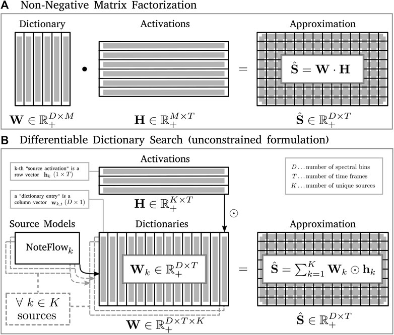
FIGURE 1. This figure illustrates decomposition of an input spectrogram S via two different methods, giving the shapes, sizes, and interactions of their different components. (A) is the standard NMF framework, while (B) shows the DDS method—in its initial, frame-level, unconstrained formulation as described in (Marták et al., 2021). The matrix of latent codes Z, columns of which are used by the source models to generate the corresponding dictionary entries in W, is omitted in favor of clarity.

An analogous decomposition, implemented by the initial formulation of the DDS method (Marták et al., 2021), is shown in Figure 1B. As can be seen, using the frame-level decomposition objective that grants each time frame in S its own unique dictionary entry for each possible source, yields a very resource-intensive decomposition structure. Each of the K possible sources has an associated generative density model, which generates a dictionary W_k of a shape equal to that of target spectrogram S, and subsequently guides its “search” during the decomposition. The scalar values in the activation vectors h_k are used to scale the individual dictionary entries in W_k. Summing the result across all K sources completes the linear combination of the non-linear differentiable dictionaries².

3.2 Proposed modifications

In the first step towards reducing computational demands and constraining the excessive flexibility, we fix the number of dictionary entries used for each source to a constant—a free parameter of the method, called “components per source”, that can be specified by the user—by introducing the matrix multiplication structure from the NMF framework, and bridging one fundamental gap between the two methods. The generated dictionary entries can now be reused over time. This means that the objective we minimize to obtain both the decomposition and the adapted dictionary entries, is now defined with respect to the whole input spectrogram, as opposed to its individual frames.

The second step towards improving resource utilization replaces the separate, unconditional density models with a single, conditional density model for all sources. This model combines both discriminative and generative aspects of dictionary modeling, by learning a mapping of data onto such a representation that carries information about the class identity of the source separately from the specifics of the particular sample. This considerably reduces the total parameter count used to model all sound sources, as well as reducing computational demands during decomposition. It also supports generalization through the increase in data efficiency via parameter reuse, as all of the training samples from all sources are now combined to train a single model with its unique set of parameters. Additionally, it completely removes the need to estimate the non-discriminative intervals on the likelihood axis—those parts of the likelihood space under a particular source model, where samples of the true source mix with samples of a different source—for K ⋅ (K − 1)/2 pairs of separate source models and different source samples, after they have been trained³. To improve the performance of the density model, we adapt several modifications to the architecture that is described in (Kingma and Dhariwal, 2018). The remainder of this section describes our modified approach in further detail, with an overview of the relevant components for both the basic NMF decomposition structure and the updated differentiable dictionary model in Figure 2.

FIGURE 2

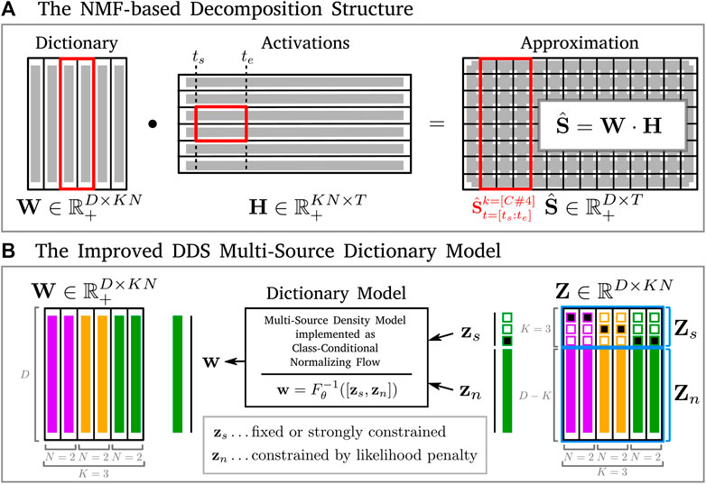
FIGURE 2. Overview of our modified formulation of DDS. Sub-figure (A) shows the adaptation of NMF decomposition, with the particular structuring of the dictionary W and activation H matrices into K sources expressed with N components each. The red frames exemplify how this structure allows one to get a reconstruction containing only activity of a particular source (e.g., note C#4) in a sub-selected time snippet (e.g., time frames from 2nd to 4th), capacity of which we will leverage in Section 5.1. (B) shows the multi-source dictionary model generating the complete dictionary matrix, as necessitated by the NMF decomposition structure in order to efficiently fuse it with the DDS framework. As opposed to the single-source multi-model approach that would project different noise vectors from Z by different single-source models to create W, expressing the source identity in the models, our multi-source model enables explicit separation of the noise vectors in the nuisance parts Z_n, from the source identity parts, which are expressed in the semantic parts Z_s of the latent codes. The “Dictionary Model” component is implemented as a normalizing flow, and the conditional sampling, as described in Section 3.4, can be performed by combining the 1-hot code of the source class z_s, with the nuisance vector that can be sampled from the model’s prior z_n ∼ p_Z(z), and projecting the result to the data space using the explicit inverse exposed by the model, as $\mathbf{w}=F_{\theta }^{-1}([{\mathbf{z}}_s,{\mathbf{z}}_n])$.

3.3 Fusing the DDS framework with the NMF decomposition structure

Let N denote the aforementioned parameter “components per source” — the number of dictionary entries that our modified DDS model will be able to use to express each one of the K possible sound sources. The representational power and adaptability of the method can be adjusted by tweaking this parameter.

Given a magnitude spectrogram $\mathbf{S}\in {\mathbb{R}}_{+}^{D\times T}$ with D frequency bins and T time frames, NMF approximates its contents as $\widehat{\mathbf{S}}=\mathbf{W}\cdot \mathbf{H}$. We will inherit this decomposition structure in our adaptation. For a decomposition with DDS, however, the dictionary $\mathbf{W}\in {\mathbb{R}}_{+}^{D\times KN}$ and activation $\mathbf{H}\in {\mathbb{R}}_{+}^{KN\times T}$ matrices are structured into K groups that correspond to individual sources, each of which encompasses N columns in W and N rows in H, jointly modeling the spectral representation and temporal activity of individual sources. After minimizing the decomposition objective, activities of source templates are distributed over their N components. We aggregate them by summing up the actitivities over these components. This results in an activation matrix of shape [K × T], representing source activity over time.

The entries of the dictionary W are obtained by transforming a corresponding set of latent codes $\mathbf{Z}\in {\mathbb{R}}^{D\times KN}$, through a bijective mapping. This mapping is implemented as a Normalizing Flow (Tabak and Vanden-Eijnden, 2010), and unifies both discriminative and generative aspects as will be outlined in the following.

3.4 The multi-source class-conditional density model

To be able to model probability densities of different sound sources with a single model, we need a conditional density model that allows explicit conditioning on the class of dictionary entry to be generated, via sampling x ∼ p_model(x|y), conditional on the source class label y. The approach described in (Jacobsen et al., 2018) is a perfect match for these requirements. It was originally designed to study the relationship between “invariances to meaningful” perturbations, and “vulnerabilities to adversarial” sample perturbations that are made to the input of deep neural networks. Both are unwanted effects, as an “invariance to meaningful” perturbation means the network is not changing the predicted class in response to a relatively large perturbation that actually changes the meaning of the input, whereas a “vulnerability to adversarial” perturbation means the network is changing the predicted class in response to an almost imperceptible, meaningless change in the input.

3.4.1 Training Procedure

A normalizing flow F_θ maps the data point $\mathbf{x}\in {\mathbb{R}}^d$ onto a latent code $\mathbf{z}\in {\mathbb{R}}^d$ of equal dimension d, as z = F_θ(x), exposing an explicit inverse mapping $\mathbf{x}=F_{\theta }^{-1}(\mathbf{z})$ by design. Given a labeled dataset with C classes, the vector z can conceptually be split by its dimension into two parts: a semantic part ${\mathbf{z}}_s\in {\mathbb{R}}^C$, and a nuisance part ${\mathbf{z}}_n\in {\mathbb{R}}^{d-C}$. With the help of a small adversary, a so called nuisance classifier network $E_{{\theta }_{nc}}$, which has a separate set of parameters θ_nc, and is only used during training, we can now describe both the objective that is minimized, as well as the procedure that needs to be followed.

Each training step contains a sub-routine preceding the computation of the main objective, and the update of θ. While the main set of parameters θ is held fixed, the nuisance classifier $E_{{\theta }_{nc}}$ is trained for a few iterations to minimize the cross-entropy $CE(\mathbf{y};E_{{\theta }_{nc}}(F_{\theta }{(\mathbf{x})}_n))$ between the true class label in 1-hot encoding y ∈ {0,1}^C, and its own class predictions from the nuisance variables F_θ(x)_n = z_n, updating the parameters θ_nc. Subsequently, the main objective is evaluated to compute the update for θ once.

The main objective combines the standard normalizing flow maximum likelihood estimation term nMLE(x) (cf. Eq. 3) — the negative log-likelihood—computed on the nuisance part F_θ(x)_n = z_n, with an adversarial objective (Jacobsen et al., 2018) called independence cross-entropy (iCE). The iCE term combines minimization of semantic cross-entropy sCE(y; σ(F_θ(x)_s)) between the labels and semantic dimensions, with maximization of nuisance cross-entropy $nCE(\mathbf{y};E_{{\theta }_{nc}}(F_{\theta }{(\mathbf{x})}_n))$ (cf. Eq. (2)) between the labels and predictions of the nuisance classifier $E_{{\theta }_{nc}}$, which also applies softmax σ to output probabilistic predictions.

During the sub-routine, the nuisance classifier E tries to predict class-specific (semantic) information from the part of the latent vector z that actually should be class-agnostic (nuisance). By maximizing the error of nuisance classifier, the conditional density model F_θ is incentivized to remove any semantic information that is still mapped to z_n, while minimizing the semantic error draws it to map it all to z_s. This adversarial objective may also be viewed through the lens of information theory, as minimizing a lower bound on the mutual information I(y; z_n), with the maximization term seeking to tighten the bound⁴.

3.4.2 Building the dictionary model

In the context of our multi-source audio modeling problem, the spectral resolution D dictates the data dimensionality, while the K sources are treated as separate classes. This splits the latent code z into two parts. The first K dimensions make up the semantic part z_s, and the remaining D − K dimensions form the nuisance part z_n.

To be able to condition the generative model on a particular sound source, we deviate from the original iCE objective by replacing the softmax output and the cross-entropy term sCE(y; F_θ(x)_s) in the objective, with a linear output and a mean squared error term sMSE(y; F_θ(x)_s) (cf. Equation 1). The reason for this change is simply that a softmax function would not be explicitly invertible, at least not without sampling. As a result, conditioning on the source identity when generating a sample is as simple as setting the semantic dimensions z_s to the 1-hot code that identifies the desired source, while sampling the nuisance z_n from the prior. The final objective combining our modified iCE with nMLE is thus given by Equation 4.

$sMSE\left(\mathbf{y};\widehat{\mathbf{y}}≔F_{\theta }{\left(\mathbf{x}\right)}_s\right)=\sum _{k=1}^K{\left(y_k-{\widehat{y}}_k\right)}^2(1)$

$nCE\left(\mathbf{y};\widehat{\mathbf{y}}≔E_{{\theta }_{nc}}\left(F_{\theta }{\left(\mathbf{x}\right)}_n\right)\right)=-\sum _{k=1}^K{y}_k\log \left({\widehat{y}}_k\right)(2)$

$nMLE\left({\mathbf{z}}_n≔F_{\theta }{\left(\mathbf{x}\right)}_n\right)=-\sum \log \left(p\left({\mathbf{z}}_n\right)|\det \left(\underset{\theta }{\overset{x}{\mathbf{J}}}\right)|\right)(3)$

$\underset{\theta }{\min }\underset{{\theta }_{nc}}{\max }\mathcal{L}\left(\theta ,{\theta }_{nc}\right)=\underset{\text{modified\hspace{0.17em}}iCE}{\underbrace{{\mathcal{L}}_{\mathit{sMSE}}\left(\theta \right)-{\mathcal{L}}_{\mathit{nCE}}\left(\theta ,{\theta }_{nc}\right)}}+{\mathcal{L}}_{\mathit{nMLE}}\left(\theta \right)(4)$

We find the relative weighting of the adversarial cost terms (sMSE and nCE) to be crucial for successfully concentrating the class information in the semantic dimensions z_s.

Finally, to further boost the modeling capacity of our unified source model, we introduce the key architectural components of the Glow architecture. Each step of the normalizing flow first normalizes the input using actnorm (Kingma and Dhariwal, 2018), a form of minibatch-independent normalization with data-dependent initialization. The shuffling of dimensions between flow steps is then carried out via an invertible 1x1 convolution (Kingma and Dhariwal, 2018), which can be seen as a generalization of the fixed, random permutations layers used in (Dinh et al., 2017). Since the 1 × 1 convolution kernel is a fully trainable linear transformation matrix without additional constraints, it can effectively learn to perform a mixing operation. We follow (Kingma and Dhariwal, 2018) in parameterizing this mixing matrix in its LU-decomposition and use no bias for this layer. Following (Marták et al., 2021), we use affine coupling layers, and discard the multi-scale architecture of (Dinh et al., 2017; Kingma and Dhariwal, 2018), which was originally devised to save computational resources when modeling high-dimensional data with 2-dimensional structure. This is because we merely need to model individual spectral frames of 1-dimensional structure, with spectral resolutions resulting in affordable resource demands⁵.

3.5 The decomposition objective

Given a conditional generative density model that generates samples as $\mathbf{x}=F_{\theta }^{-1}([{\mathbf{z}}_s,{\mathbf{z}}_n])$, we can now structure our matrix of latent codes $\mathbf{Z}\in {\mathbb{R}}^{D\times KN}$ into the semantic ${\mathbf{Z}}_s\in {\mathbb{R}}^{K\times KN}$ and nuisance ${\mathbf{Z}}_n\in {\mathbb{R}}^{D-K\times KN}$ sub-matrices. The full dictionary is then simply expressed as $\mathbf{W}=ReLU(F_{\theta }^{-1}([{\mathbf{Z}}_s,{\mathbf{Z}}_n]))\in {\mathbb{R}}_{+}^{D\times KN}$, using the rectifier activation to satisfy the non-negativity constraint of the generated samples for convenience, as alternative implementations of the projection to the non-negative orthant are possible.

We initialize the semantic parts of the latent vectors Z_s to 1-hot encodings to specify which sources we want to model, and hold them fixed during decomposition. To further increase the flexibility of the dictionary search, it is possible to allow for slight deviations from the sharp binary values with a soft constraint, but we opted not to do so for now. Section 5.2 offers further discussion of semantic conditioning in our dictionary model.

The nuisance parts of dictionary entries Z_s can be sampled from a standard normal distribution. In practice, we find that initializing them all to the zero vector 0 yields good results more consistently. We believe that this eliminates the chance of samples “spawning in the wrong volume of the latent space”.

The DDS decomposition of an input spectrogram S ≈ W ⋅H is then obtained by minimizing the objective $\mathcal{L}$ (cf. Equation 5) by alternating updates of H and Z_n, following the gradients $\frac{\partial \mathcal{L}}{\partial \mathbf{H}}$ and $\frac{\partial \mathcal{L}}{\partial {\mathbf{Z}}_n}$ respectively.

$\mathcal{L}=\Vert \mathbf{S}-\widehat{\mathbf{S}}{\Vert }_2-\sum \log p\left({\mathbf{Z}}_n\right)(5)$

For the sake of clarity, we omit the complex weighting scheme of the likelihood penalty term in Eq. 5. The global weighting of the total likelihood penalty after summation is complemented by a local weighting of each dictionary element’s likelihood before summation, via their time-aggregated frame-wise relative activity contributions in H. It was devised to allow the likelihood penalty term to be appropriately balanced with the temporally aggregated reconstruction error, allowing each dictionary element a penalty contribution proportional to the “amount” of input it is used to explain.

This particular weighting scheme, conceptually following and adapted from (Marták et al., 2021), is not a result of exhaustive search, but rather merely one of many possibilities that we ended up using in our experiments, and is therefore subject to further scrutiny. It is, however, fully described by the source code accompanying this paper.

3.6 Impact on resource efficiency and performance

Coming back to the aforementioned disadvantages of the original approach, we should note that the optimizations introduced in our reformulation above were directly motivated by our experiments attempting to scale up the original formulation. Despite being able to train and evaluate the original approach on 5 octaves of piano sounds, we have seen the linear growth of complexity in both sources K and time T quickly become burdensome computation-wise, while the excessive dictionary capacity allowed unnecessary errors to accumulate.

More specifically, to highlight the difference in performance between the two formulations, let us inspect their most expensive component—the dictionary modeling. Let U denote the number of matrix multiplications involved in a single forward pass in a normalizing flow used as a source model. The matrices have shapes approximately on the order of (batch × D) for the data, and (D × D) for parameter matrices. To generate the dictionary, the original approach uses K models, each of which processes a batch of T samples, while our optimized variant uses one model to process a single batch of KN samples (where N is the number of components per source–defined in Section 3.3 above). In terms of the raw cost of the matrix multiplications, this yields an improvement from K ⋅ Θ (TD²) ⋅ U to Θ(KND²) ⋅ U in time, and from K ⋅ Θ (TD + D²) ⋅ U to Θ(KND + D²) ⋅ U in space complexity. By fixing the number of dictionary entries, we have reduced the linear time complexity factor in input length T to a constant N, which is the most significant improvement, especially because it factors into the quadratic cost in spectral resolution D². By replacing K models with a single one, we have reduced the memory complexity by (K − 1)D², as much fewer parameters need to be held in memory for the dictionary search-related updates. Given a constrained memory budget⁶ and a 10 min long audio recording, we measured the wall clock time cost of its decomposition by both the original, and our optimized formulation, and found an average iteration cost of 72.8 s (original), and 2.4 s (optimized), with both iteration costs averaged over 1,000 iterations. This is a $\approx 30$-fold speed-up.

Additionally, we have also seen improvements in terms of decomposition performance, as the two introduced changes both reduce the excessive flexibility of the original model: (i) by limiting the number of dictionary components and allowing their re-use, and (ii) by concentrating the use of all relevant training samples to optimize parameters of the unified dictionary model, improving overall generalization potential. A small-scale quantitative performance comparison as well as an asymptotic complexity comparison for different components of multiple method variants can be found in Marták et al. (2022).

4 Results

To test the behavior of our modified approach, we make use of the MAPS dataset (Emiya et al., 2009), as it provides the necessary variety of recording conditions as well as musical and non-musical content that allows us to study certain aspects of the problem in isolation. We describe the specifics of our experimental setup in Section 4.1, report on quantitative performance in Sections 4.2, 4.3 for non-musical and musical signals, respectively, and present qualitative analysis in Section 5.1.

4.1 Experimental setup

4.1.1 Data

The MAPS (MIDI-Aligned Piano Sounds) dataset (Emiya et al., 2009) is a collection of piano recordings with temporally aligned MIDI annotations that has been designed to support evaluation of various MIR research problems, and has often been used in the literature for evaluating Multi-Pitch Estimation (MPE) as well as AMT algorithms. It is structured into 4 subsets: the ISOL set contains isolated notes, the RAND set contains random note combinations, the UCHO set comprises “usual” chords from Western music, and the MUS set contains 30 pieces of classical piano music for each set of recording conditions⁷. Each of these subsets is further sub-divided into sample recordings made with different instrument models in various recording conditions. This particular aspect of MAPS makes it well suited for our evaluation, as we can use samples with different timbre and recording conditions for training and evaluation, while controlling for other parameters, in order to emulate the problem scenario of realistic transcription that we investigate.

To train the multi-source conditional density model, we use only those parts of the ISOL subset of MAPS that contain isolated notes synthesized using software samplers. The other parts of the RAND and MUS subsets that were recorded from a Yamaha Disklavier piano are used for testing. The RAND subset was generated by drawing notes uniformly at random from a given range, with varying degrees of polyphony and levels of intensity. That is why we will use it to benchmark performance of transcription systems on non-musical piano sounds (note combinations) in Section 4.2. Comparing this to the models’ performance on the MUS subset (Section 4.3), which we take to represent typical musical piano sounds, we can now gain insights about their respective susceptibility to the problem of corpus bias acquisition.

Additionally, we work exclusively with data from the note range M36-95 (the range of central five octaves, from C2 to C7), and exclude samples that use the sustain pedal. In the context of our spectrogram decomposition framework, each note within this range is considered a separate sound source.

4.1.2 Audio processing

The MAPS audio samples are encoded as 44.1 kHz stereo WAV files, accompanied by temporally aligned symbolic ground truth in the form of MIDI files. Before computing spectrograms, we downsample the recordings to 16 kHz mono waveforms. For spectral analysis, we use a DFT window size of 2048, a hop size of 512 samples and the Hann window function, resulting in a frequency resolution of 1,024 spectral bins, capturing frequencies up to 8 kHz. The magnitudes of spectral activity are normalized to the interval [0; 1] and projected to logarithmic scale. We use a reversible data-independent normalization-logarithmization scheme, which first normalizes spectral magnitudes by

$\mathbf{S}=\frac{2\cdot \mathbf{S}}{\sum Hann\left(2048\right)},(6)$

and then logarithmizes the features on this scale as

$\mathbf{S}=\frac{\log \left(1+\mathbf{S}\cdot str\right)}{\log \left(1+str\right)}.(7)$

The parameter str controls what we call “logarithmization strength”, and we use value of str = 10⁴ in all our experiments.

Modeling spectral features in this form has several benefits. First, normalizing flows, as much as any other class of deep neural network models, have been shown to perform better on normalized data. Second, the spectral components of the harmonic overtone series specific to musical sound sources get amplified within the logarithmic domain of features, which helps the models capture their behavior, and separate them from the ‘noise’. This can be seen as a means to control the signal-to-noise ratio in the features of magnitude spectra.

Using such a reversible projection leaves an opportunity to project spectrograms generated by our models into their corresponding un-normalized form on linear scale. From there, one can simply use an arbitrary phase approximation method in order to arrive at audible sound excerpts from these generated spectrogram samples, by transforming them with the inverse DFT.

4.1.3 Models in comparison

In order to evaluate and highlight certain properties of interest of our new method, we will put it in context with a related linear matrix decomposition method, and a trained model from the recent literature that represents the current state of the art in (full) polyphonic piano note transcription. In addition, in Section 4.3 we will cite performance measures from other, only partly comparable models from the literature (see Table 1 there).

TABLE 1

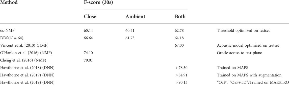
TABLE 1. Average performance across the first 30 s of the classical pieces contained in the MUS subset of MAPS—played on the Yamaha Disklavier in Close and Ambient recording conditions. The F-score metrics for DDS and the NMF baseline were calculated from binarized activations using oracle thresholds (see Section 4.1.6). The F-score for the deep neural network baselines were all calculated using fixed thresholds of 0.5.

4.1.3.1 The overcomplete NMF baseline

To assess the improvements in decomposition performance that we expect as a result of our non-linear source modeling, we will compare to an overcomplete semi-supervised NMF baseline. “Overcomplete” refers to the fact that each source will be represented in the dictionary W by the set of all training and validation samples, that are otherwise also used for training and model selection of the DDS dictionary source model. With the dictionary W fixed and only activations H adapting during the decomposition, this formulation will allow us to see the differences between the respective linear and non-linear extrapolation capacities, as the remaining properties between this baseline and our DDS formulation are similar. In this regard, we follow the comparison made in (Marták et al., 2021) as closely as possible. We expect to find the increased capacity of DDS to model unseen sources, to have positive effects on the decomposition performance relative to this baseline. In the following, we will call this model simply “NMF” for short.

4.1.3.2 The “onsets and frames” model

As a third point of comparison, we chose a model that can be considered representative of the current state of the art in polyphonic piano note transcription, in terms of recognition performance: the “Onsets and Frames” transcription system by Hawthorne et al. (2019), which was trained on the MAESTRO dataset. For this model, we will use the author provided code, as well as the model checkpoint that they generously made available⁸. Please note that the MAESTRO training set is approximately 10× larger than the MAPS training set, and about 170× larger than the set of isolated notes we used to train DDS. Furthermore, the model is geared towards a somewhat different task: rather than framewise polyphonic pitch identification, it transcribes entire notes (onset, offset, key, volume). It is also much more complex and sophisticated than our simple model. In particular, it involves task-specific temporal post-processing routines conditioned on the onsets of individual notes. Any experimental comparison will thus have to be taken with a grain of salt.

4.1.4 Training

To train our unified conditional density model that generates the dictionary entries, we use the modified 1-dimensional Glow architecture as described in Section 3.4. The model is built with 32 flow steps. Each affine coupling layer is parameterized as a multi-layer perceptron with 3 densely connected layers of 2048 units, using the LeakyReLU activation function. The Adam optimizer (Kingma and Ba, 2014) is used with the learning rate set to 1 ⋅ 10^–5 for up to 2,500 epochs with a minibatch size of 512, and an early stopping patience of 100 epochs. We compute the average log-likelihood on 20% of the training data that we set aside for validation purposes and early stopping.

For the overcomplete variant of NMF that we compare the proposed method to, we construct the dictionary W from all training samples, including the 20% of data, which is held out for validation in the training of the DDS dictionary model. This means that NMF has a small advantage in terms of direct access to data, compared to DDS.

4.1.5 Decomposition

For an NMF dictionary W with M components, the activation matrix H is initialized to $\frac{1}{M}$ everywhere. For DDS, the differentiable dictionary Z is initialized according to the description in Section 3.5, while the activation matrix H is initialized to small, random numbers in the range $[0;\sqrt{\frac{\bar{\mathbf{S}}}{KN}}]$, where $\bar{\mathbf{S}}$ denotes the grand average of the whole spectrogram matrix S.

During decomposition, we use a step size of 1 ⋅ 10^–2 for NMF and 1 ⋅ 10^–3 for DDS. The global likelihood weight c is set to 1 ⋅ 10^–4. Each decomposition is run for at most 1,000 iterations. We follow the early stopping conditions as described in (Marták et al., 2021), but do not find them triggered in our experiments.

4.1.6 Calculating metrics

To make framewise evaluation as objective as possible, we tried normalizing the dictionary entries to equal-length vectors (for both NMF and DDS), such that the values of H are on comparable scales of activity contribution, in terms of explained magnitude spectral energy. Enforcing equal norms of vectors after each step proved to heavily burden the optimization in DDS by disrupting the dynamics of dictionary search. Also, such a basis re-normalization strategy has been shown to be suboptimal in sparse NMF, at least for sound separation (Le Roux et al., 2015), compared to incorporating the normalization into the parameterization of W directly.

We choose to keep the dictionary norms free, and as a remedy, when computing metrics, we first re-scale each scalar activation in H by the norm of its corresponding dictionary vector from W, the one that is “activated” by it. Only afterwards is the activity of sources summed up across their components. This is a cheap way to express the activation values in H on a consistent, W-independent scale. In Section 5.1, we will refer to such W-norm-scaled version of the activation matrix as H_score.

When computing the F-score metric from the thresholded activation matrix H for our results in Section 4.3 we assume the existence of an oracle (in the form of the ground truth), that enables us to compute the optimal threshold in terms of F-score for each snippet. This is done so we can compare the decomposition quality of both methods in terms of familiar metrics, while avoiding any variance in performance measures that would be due to the thresholding technique. We include it merely to enable a fair comparison to the state-of-the-art, deep neural network baseline.

In order to control for the effects of the thresholding method, we compute and report the area under the precision-recall curve (AUC-PR), as a general quantifier of the upper bound on performance in terms of frame-wise AMT metrics. This relates to the fact that frame-level pitch labels are heavily imbalanced, due to most notes being inactive most of the time. Since we generally care more about the positive class (active notes) in an AMT problem that is generally sparsely labeled, AUC-PR as a quantifier of average precision is a well-suited metric.

Finally, we also report the reconstruction error (RE) of a frame, defined as the mean absolute error summed over frequency and averaged over time $\mathrm{R}\mathrm{E}(\mathbf{S},\widehat{\mathbf{S}})=(\sum \text{abs}(\mathbf{S}-\widehat{\mathbf{S}}))/T$. Alternatively, one could average over both the time and frequency dimensions, to get the average error for a single time-frequency bin. However, since we use constant spectral resolution throughout the reported results, we choose to report the average frame error.

4.2 Evaluation on non-musical piano sounds

The samples of random note combinations in the RAND subset of MAPS come in two different ranges of loudness: 60–68 (mezzo-forte) and 32–96 (from piano to forte).⁹ The samples with smaller dynamics range (only mezzo-forte notes) could be taken to correspond to a typical chord situation, where all notes are played together with similar intensity. The samples with a larger dynamics range (notes ranging from piano to forte) may represent the polyphonic music scenario where several melodic lines mix together more heterogeneously. The samples also come in 6 different polyphony levels ranging from P2 to P7.

As mentioned in Section 4.1, the spectral decomposition methods (DDS and NMF) in our comparison were trained using only samples from the ISOL subset of MAPS, while the deep neural network approach was trained on the considerably larger MAESTRO dataset, which gives it a certain advantage with respect to musical content. Each of the testing snippets used in this evaluation is created by concatenating the active parts from the relevant files of the used subset of MAPS, where notes are being played, to avoid spending compute time on silence. In a separate experiment, we tested the propensity of the compared methods to produce false positives on the parts that were cut out, and conclude that all methods behave similarly, with no false positives for silent parts.

We evaluated our modified DDS model together with an overcomplete NMF baseline on the samples with both dynamics ranges separately, and measured consistently higher performance of both methods on the samples with smaller dynamics range 60–68. This result confirms the intuition that recognizing soft notes in a mixture that may also include loud ones, is a more difficult problem. In Figure 3, we report results for the harder scenario, using samples with larger dynamics range 32–96, showing the aggregated metrics for different polyphony levels separately. We used samples of Disklavier (Dk) piano recorded in “Close” (Cl) microphone conditions, identified via instrument code ENSTDkCl within MAPS.

FIGURE 3

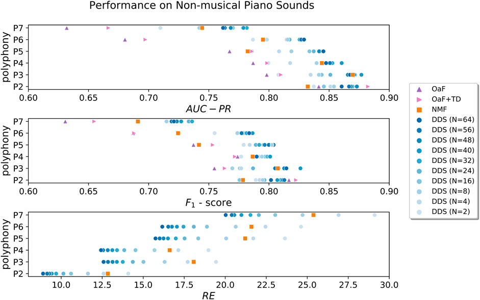
FIGURE 3. Frame-level pitch identification performance of the three methods (DDS, NMF, and OaF), quantified in terms of the AUC-PR metric and F-score, is shown in the top and middle rows of the figure. The reconstruction error of the two spectrogram decomposition methods is additionally assessed by the RE metric in the bottom row. Our new formulation of DDS is evaluated multiple times, for a set of different values for the components per source parameter N, introduced in Section 3.3. Remember that it can be viewed as controlling the “flexibility” or “representational power” of the method. The darker shades of blue would then correspond to larger representational power. This allows us to examine its influence on the two aspects of method behavior.

The framewise pitch identification performance comparison of the DDS method with the NMF baseline in the top row of Figure 3 is accompanied by performance numbers for the state-of-the-art “Onsets and Frames” system (OaF, OaF+TD), which we introduced as our second baseline above (see Section 4.1.3.2). The bottom row of Figure 3 features comparison of reconstruction performance, which is only relevant to the two spectrogram decomposition methods.

Unsurprisingly, across all methods in all three metrics (AUC-PR, F-score and RE) we see a dependency of performance on the degree of polyphony. As performance decreases with increasing polyphony level, the latter can be viewed as the determining property of the problem complexity.

We note that DDS appears to consistently outperform the linear NMF baseline across all metrics, with larger margins at higher polyphony levels, hinting at the possibility that its superior source modeling capacity is more useful in more complex problem scenarios. This can be seen as evidence for the improved capacity of DDS to deal with unseen sources, because the Disklavier instrument used in our testing samples has not been seen by either method during training. In particular, the more “flexible” parameterizations of DDS (those with higher values of N) appear to consistently improve the reconstruction performance (RE). However, this does not seem to be the case for the frame-wise pitch identification performance, as assessed by the AUC-PR and F-score metrics. Even though DDS generally performs better at higher capacity settings, the largest N parameterizations do not always translate into the best decomposition results (i.e. the darkest blue dots in the AUC-PR and F-score subplots of Figure 3 are not necessarily the rightmost ones).

Our interpretation of this is two-fold. On the one hand, the superior representational power of DDS clearly benefits the overall transcription performance potential. It most certainly does allow the method to explain increasingly larger amounts of magnitude spectral energy, reducing the reconstruction error as a result. Nonetheless, this flexibility can be a double-edged sword, as too much of it can have detrimental effects on performance. We have seen this in a separate set of experiments with the initial, unconstrained formulation of DDS, where the dictionary adaptation is overall much less constrained, as its entries are not reused over time. In a degenerate case, the DDS model finds ways to misuse its spare capacity, explaining leftover residual energy of the magnitude spectrum with “un-exhausted” dictionary components of arbitrary sources. This ends up reducing the reconstruction error at the cost of impairing pitch identification accuracy. In theory, this may happen whenever the gains achieved in reconstruction performance do not get outweighed by the likelihood penalties associated with the misused dictionary components, as they should. This, in turn, may point towards imperfections in the model, or the weighting of the likelihood penalty.

We identify three fundamental handles through which a practitioner of the DDS method can attempt to control the extent to which its modeling capacity is used to their benefit: (i) tweaking N to adjust $\frac{N}{T}$ — the ratio of number of components to number of time frames across which they may be reused; (ii) adjusting the global likelihood penalty weight, in an attempt to strike a balance between the incentive to explain magnitude activity and the incentive to explain it correctly; and (iii) the rather more abstract behavior of the trained source model, which can be inspected and addressed by assessment of such qualities as generalization or discriminative performance. In Section 5.1, we will see an example of such malfunction in Figure 4, demonstrating a particular way to draw actionable insights from the model, by leveraging its modular nature.

FIGURE 4

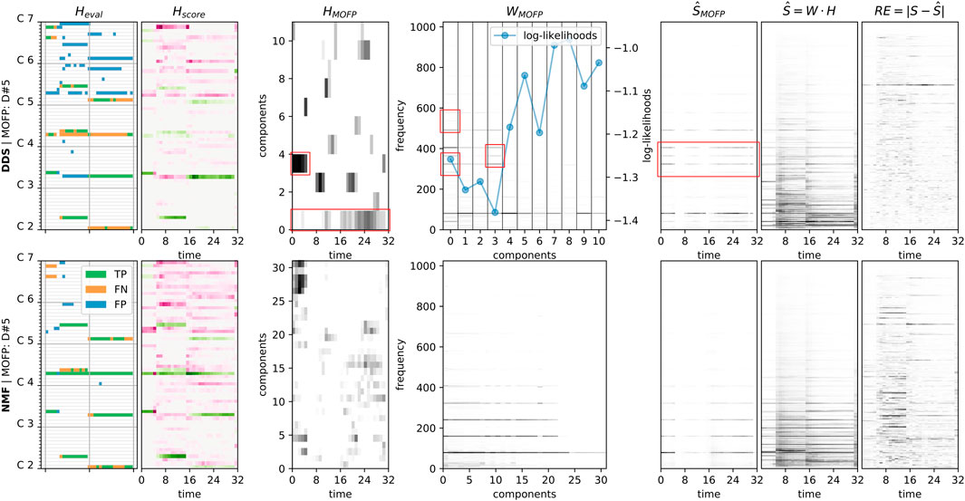
FIGURE 4. In this figure, we juxtapose the components of interest to inference of frame-level transcription of short spectrogram snippet of 32 frames, by two decomposition methods. The top row shows DDS, the bottom NMF. The columns, introduced from left to the right, have the following contents: 1) H_eval is the evaluation matrix based on oracle threshold (threshold computed using ground truth labels, such that highest potential F-score is reached) computed by thresholding H_score; 2) H_score contains source-aggregated activity of H, after re-scaling by the norms of W, related to ground truth through color (green for correctly attributed activity, purple for mis-attributed activity); 3–4) subsets of the activation matrix H_MOFP and of the dictionary W_MOFP showing the active components (the ones with total activity above 0.05) of the Most Offending False Positive (MOFP) note—found as a note with the highest total mis-attribution of activity (purple color in H_score summed across time frames), ordered by total spectral energy of the component (calculated as sum across frequency components), ordered from highest to lowest in terms of total spectral energy, for better clarity; 5) part of the approximation $\widehat{\mathbf{S}}$ generated by the sub selected components of the MOFP note—as illustrated by the red framing in Figure 2A; 6) full approximation of the snippet $\widehat{\mathbf{S}}$; and finally 7) reconstruction error.

Finally, and perhaps quite surprisingly, we observe that the state-of-the-art, deep neural network baseline (OaF, OaF+TD) performs worse than linear decomposition methods on these unusual chords, at least for a degree of polyphony greater than two. We conjecture that due to the large shift between the distribution of note combinations occurring in classical piano music (which the neural network was trained on), and the uniform distribution used to generate note combinations in the test data, we can see evidence of the corpus bias we mentioned before. As the amount of possible (random) two combinations is far smaller than for greater degrees of polyphony, and therefore also has much greater coverage in musical corpora, we can observe the neural network outperforming the decomposition-based methods for P2. Perhaps, then, this result is only surprising in the context of how these systems have always been evaluated: using musical pieces of the same genre (or musical style) as the pieces used for training, where the genre property encompasses the specific distribution of note combinations. In this more typical evaluation scenario involving musical pieces (see Section 4.3), the deep neural network-based models consistently outperform their decomposition-based counterparts, as their bias towards musical content is actually beneficial in this scenario.

Regarding the evaluation of the state-of-the-art “Onsets and Frames” polyphonic piano transcription model (Hawthorne et al., 2019), denoted by “OaF” and “OaF+TD” in the first and middle rows of Figure 3, there are a few things to note. In order to compute AUC-PR and maximum attainable F-score, we had to modify the provided code. The binarization thresholds for onset, frame and offset output heads were originally set to a constant 0.5, and then post-processed with a straightforward, hard-coded, temporal decoding routine. We modified the code slightly, in order to change the three aforementioned binarization thresholds simultaneously, and only subsequently run the temporal decoding routine afterwards. In the interest of fairness, we evaluated the neural network model twice: with and without temporal decoding, referred to by “OaF+TD” and “OaF” respectively in Figure 3. We did this for the following reason: due to the nature of the temporal decoding routine, which is fully dependent on an onset being present, the AUC-PR and F-score values might have been unduly influenced by detection errors propagated over time. As we can see from the performance numbers, our concerns were largely unnecessary, as it appears that the temporal decoding step improves over the framewise result for almost all degrees of polyphony.

4.3 Evaluation on musical piano sounds

We now turn to the evaluation scenario where the test snippets contain musical piano sounds, coming from the MUS subset of MAPS, while the training material—except for the Deep Neural Network (DNN) based methods (Hawthorne et al., 2018, 2019) — is still isolated notes (MAPS/ISOL). Let us reiterate that the samples of isolated notes used to train NMF and DDS were all selected to contain all the other instruments than the Disklavier—the synthesizers. On the other hand, the testing pieces used for evaluation were all selected to contain only the Disklavier. Thus, the realistic transcription scenario, where we evaluate on previously unseen sources, fully applies to our results in Table 1. In fact, this particular split strategy corresponds to configuration II in (Sigtia et al., 2016).

Since the DDS and NMF methods are both restricted to the sources in the 5 central octaves of piano claviature (C2-C7), any labels outside of this range (of which there are very few) are excluded from the metric computations. In cases where spectral activity produced by a note outside of this range occurs, the compared decomposition methods are at equal disadvantage when presented with the challenge of explaining this activity somehow. This naturally decreases their performance globally, but does not impair the quality of their relative comparison. We report the measures averaged over the pieces in Table 1. Please do note the comments in the last column of Table 1 that outline the many differences between train/test protocols, which make many of the measures not directly comparable.

First, we observe that the DDS approach outperforms the NMF baseline on musical signals by slightly smaller, but generally similar margins, as on the non-musical ones shown in Figure 3. We conjecture that the lower performance of both methods on real music can be attributed to certain intuitive musical differences between the tasks: real music may contain larger note dynamics ranges, especially with different parts of various notes overlapping, as well as generally higher levels of polyphony.

Multiple variants of an adaptive decomposition method with harmonic constraints on the dictionary are described in (Vincent et al., 2010), and for Table 1 we picked the highest F-score that is reported. This result is not readily comparable to others, however, as the authors state that all parameters of their harmonic constraints were optimized on the testset (to facilitate a fair comparison of the potential of their approach and reimplementations of other approaches). The method proposed in (O’Hanlon et al., 2016) learns its dictionary specifically from isolated notes recorded in the same acoustic conditions as the musical pieces it is tested on. Similarly, the “Attack/Decay” temporal post-processing approach proposed in (Cheng et al., 2016) achieves a rather high F-score, while also learning their dictionary from isolated notes of the piano in the testset. Given that all the NMF based methods in the table either use information that is unavailable to DDS or the NMF baseline we chose, or whose adaptive acoustic models are tuned to maximize performance on the testset, this essentially makes a fair comparison nigh impossible.

If we now compare the performance of the proposed, modified DDS approach and the best performing deep neural network-based system (“Onsets and Frames”, “OaF”) that is described in (Hawthorne et al., 2019), the performance gap is almost $\sim 27$ percentage points in frame-wise polyphonic pitch detection performance on the MAPS MUS subset.

To summarize: for classical music, as represented by both the MAPS and MAESTRO datasets, all deep neural network-based solutions outperform DDS by a very large margin. Yet, even the system that was trained with more than 170 h of polyphonic piano data still struggles with “unusual chords”, as shown in Figure 3 in Section 4.2. We take this as strong empirical evidence that the “corpus bias” problem that was initially outlined in (Kelz and Widmer, 2017) is not yet solved, and simply increasing the amount of training data with additional music will most likely not fix it. Let us assume, we were to try to remedy the situation, and “just include all unusual chords during training”. Such approaches face a combinatorial explosion of possible chords with a (very conservative) lower bound of ${\sum }_{k=0}^5\left(\genfrac{}{}{0ex}{}{88}{k}\right)\approx 41.6\cdot 10^6$, where we assume that the degree of polyphony is restricted to a maximum of 5 notes (two or three fingers playing per hand, no pedal). If we go on and assume that each individual chord is recorded for about half a second, this would amount to roughly 5,780 h of extra training data for this rather simplistic scenario alone.

5 Additional insights

In this section, we report on some additional experiments and investigations that should give some further insights into the workings and potential of the proposed method.

5.1 Model transparency

The following example attempts to demonstrate the benefits of the innate transparency of our modified DDS model. The modular nature inherited from the NMF decomposition structure, along with the explicit-likelihood multi-source dictionary model with source conditioning, enables its practitioner to relatively straightforwardly trace an error on the output of the system towards its source.

The example presented in Figure 4 shows decompositions of a 1-second-long snippet from the MAPS/RAND samples that was deliberately chosen to showcase the statistically least common situation—one in which the DDS model significantly underperforms its NMF baseline. In particular, the AUC-PR of the DDS decomposition shown in the upper half of the figure evaluates to only 40.51, as opposed to the NMF decomposition shown in the lower half, which scores 85.14. This corresponds to the biggest DDS underperformance of the NMF baseline that can be found among our MAPS/RAND decompositions. We use this example to show how simple it is to spot “what went wrong”.

As per the caption of Figure 4 describing its individual components, the evaluation against ground truth in H_eval is computed from the H_score matrix after thresholding with oracle thresholds (see Section 4.1.6). The subset of DDS dictionary entries detailing only the “most active” (see figure caption) components of the note which was responsible for the “most offending false positive” (see figure caption) — shown in the matrix W_MOFP along with its activations H_MOFP and resulting part of approximation ${\widehat{\mathbf{S}}}_{\mathit{MOFP}}$ — reveals the issue. Specifically, the two dictionary components indexed by 0 and 3 contain spectral activity in between the true harmonic partials of the source in question, which is clearly misplaced, as highlighted by red colored bounding boxes in the figure. A practitioner of the DDS method can take this insight and use it, for example, to elaborate an investigation into the behavior of their source model, or alternatively, into the current balance between the likelihood constraint term and the reconstruction error term, in the objective of the optimization.

This can be related to the example of note comprehension as a concept, examined by (Kelz and Widmer, 2019) in an invertible transcription neural network (cf. Figure 7 in (Kelz and Widmer, 2019)). As opposed to the end-to-end approach of (Kelz and Widmer, 2019), the linear mixing assumption of our model allows us to use transcription errors to automatically identify possible failures of our note model in grasping how a particular note should look like.

5.2 Conditioning the sampling and search

When it comes to conditioning our generative model on the class labels of samples (to express the differentiable dictionary in our DDS formulation), we simply fix the semantic dimensions to 1-hot vectors according to the class labels, and keep them fixed as we “search” the dictionary. We take the testing samples of isolated notes from the Disklavier instrument (unseen during training), and inspect how closely they land around their intended binary coordinates, in the semantic part of the latent space, after projection through our multi-source model.

By using the conditioning mechanism described in Section 3.4.2 for dictionary adaptation, we are practically making the following set of assumptions:

1. The training procedure succeeded in concentrating the class information in z_s by tightening the lower bound on the minimized mutual information I(y; z_n) sufficiently: and

2. The training procedure succeeded in minimizing the semantic error term sMSE all the way to zero

As a result, we expect the model to generalize to unseen sources in a way that any novelty in intra-class feature variance—such as a previously unseen timbre—will be mostly captured by novel variance in the nuisance dimensions of the model’s latent space $\mathcal{Z}$. However, considering the nature of the learning algorithm applied and the function class used to do the approximation, some margin for generalization error necessarily needs to be considered.

In particular, since the model architecture used to express the bijective mapping F_θ between the data space $\mathcal{X}$ and latent space $\mathcal{Z}$ is a normalizing flow, the function it learns is an instance of a diffeomorphism—a smooth map between two smooth manifolds—with all dimensions of the two spaces mutually interacting through the map. As a result, even in the case of highly successful learning with our modified iCE objective (Eq. 4), some amount of intra-class data variance should still be expected to be “leftover” mapped onto the semantic dimensions z_s, possibly within a small neighborhood of the exact 1-hot semantic code of the given class.

In the following, we inspect the behavior of the conditional density model that was used for all of the DDS experiments reported throughout this manuscript. We used this model F_θ, to project all samples from the held-out test set of all notes in the modeled range (C2-C7), onto the latent space $\mathcal{Z}$, and report on values of semantic dimensions z_s to see how much they deviate from their 1-hot binary labels y ∈ {0,1}^K. The results are shown in Figure 5 as a histogram with the counts on a logarithmic scale.

FIGURE 5

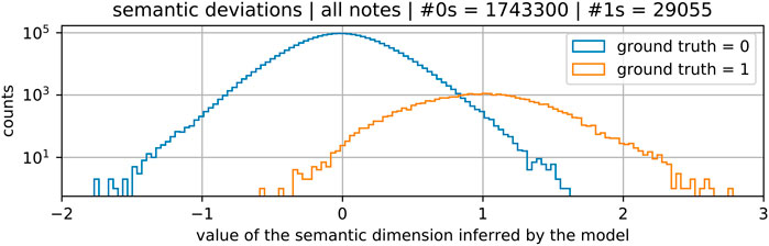
FIGURE 5. Histograms of scalar values found in the semantic dimensions z_s inferred by our multi-source model F_θ from the set of testing samples of isolated notes x coming from ISOL subset of MAPS. The multiple orders of magnitude difference between the total counts of zeros and ones, as indicated in the figure title, stems from the nature of 1-hot labeling. The blue histogram shows counts of numbers that should be “landing on” 0s, according to the labeling, while the orange one shows counts for the 1s, as indicated in the legend. The logarithmic scale of the histogram counts allows for direct comparison of relative rates of displacements for the two types of indicative dimensions, despite the large discrepancy in total counts.

Keeping in mind the logarithmic scale of the vertical axis, the slight difference in shapes of the two ‘bells’ indicates higher relative rates of larger deviations from 1s, than those from 0s. We hypothesize that the flexibility of dictionary search could be additionally increased simply by allowing a certain bounded amount of deviation from the ground truth 1-hot code, within the semantic dimensions z_s. However, in order to devise an approach that would allow the DDS method to capitalize on such increased flexibility without impairing its performance by introducing more potential for finding degenerate solutions, it will be necessary to further study the dynamics of such a trained model.

6 Conclusion

We proposed a modification of a recent audio decomposition method (DDS), in order to allow its application to the task of framewise polyphonic piano transcription, and introduced a way to constrain its flexibility at the time of decomposition. We compared its transcription performance to an overcomplete variant of NMF under almost equal conditions, with NMF being slightly favored in terms of available training data. The experiments were designed to evaluate the raw performance potential of the method, without introducing specialized constraints that boost performance by leveraging task domain knowledge. Our experimental results show the potential of DDS for polyphonic transcription. The method manages to successfully integrate the high modeling capacity of deep generative models into the NMF framework, without sacrificing explainability. We also demonstrated the mechanism of interpretability, by which the prediction errors made by the DDS model can be subjected to scrutiny. Additionally, we showed that existing frame-wise piano transcription systems based on deep end-to-end neural networks strongly suffer from corpus bias–a bias towards the note combinations encountered the most in the training corpus. Thus, we hope to have demonstrated how deep, high capacity non-linear models can be applied to frame-wise polyphonic piano transcription, without introducing corpus bias.

Obviously, this is only a starting point, and the DDS method is still limited in several respects. The upper bound on its performance is conceptually given by the discrepancy between the linear mixing assumption and the non-linearity of magnitude spectra feature space. To some extent, this can be potentially improved through the use of increased spectral resolutions, which reduces the amount of problematic feature overlap stemming from the aforementioned discrepancy. Higher spectral resolution, however, comes with increase in computational cost, and is further limited by the capacity of the dictionary model to correctly capture the feature space arising from those spectral resolutions. This could be addressed by further improving computational efficiency and modeling capacity of the used source model. In any case, the variant evaluated in this work is a “bare” one. Whether at the level of dictionary modeling, regularizing decomposition objectives, or sophisticated post-processing techniques, plenty of avenues to boost its transcription performance remain open for future exploration.

Data availability statement

The original contributions presented in the study are included in the article/supplementary material, further inquiries can be directed to the corresponding author.

Author contributions

LM and RK jointly developed the DDS models; LM carried out the implementation and all of the experimental work; GW provided supervision throughout; LM, RK, and GW jointly wrote the paper.

Funding

The LIT AI Lab receives funding by the Federal State of Upper Austria. GW’s work is supported by the European Research Council (ERC) under the EU’s Horizon 2020 research and innovation programme, grant agreement No. 101019375 (“Whither Music?”)-.

Conflict of interest

The authors declare that the research was conducted in the absence of any commercial or financial relationships that could be construed as a potential conflict of interest.

Publisher’s note

All claims expressed in this article are solely those of the authors and do not necessarily represent those of their affiliated organizations, or those of the publisher, the editors and the reviewers. Any product that may be evaluated in this article, or claim that may be made by its manufacturer, is not guaranteed or endorsed by the publisher.

Footnotes

¹This particular aspect of the highly controlled experiment design was motivated strictly by the objective to quantify direct effects of the non-linear extrapolation capability of DDS, when juxtaposed against an over-complete NMF baseline that is equipped with merely linear capacity to extrapolate from the basis. It is also what makes scaling this formulation up to a more practical problem scenario–such as piano music transcription–extremely difficult and expensive.

²For an insightful illustration of how DDS approximation of individual spectral frame could look like for piano music—including certain details (which are omitted from Figure 1B in the interest of clarity) of the generative source model—an interested reader may look at Figure 2 in (Marták et al., 2021).

³This needs to be done in the original approach in order to quantify the potential for confusion of one source with another, potentially similar source, during the dictionary search, with implications for calibrating the global weight coefficient applied to scale the likelihood penalty term in the decomposition objective. Demonstration of such quantification can be found in Section IV.B of (Marták et al., 2021).

⁴An interested reader may refer to Lemma 10 in Appendix C of (Jacobsen et al., 2018).

⁵Nonetheless, a 1-dimensional analogue of the multi-scale architecture can be devised and applied, in the interest of further computational cost optimization.

⁶We used a single GeForce RTX 2080 Ti GPU with a VRAM capacity of 11GB.

⁷For each set of recording conditions, the 30 pieces were randomly selected from a set of about 238 pieces, available at the time of database creation in the online collection of “Classical Piano MIDI files” at http://www.piano-midi.de. Therefore, some of them were chosen into several sub sets.

⁸https://github.com/magenta/magenta/tree/main/magenta/models/onsets_frames_transcription

⁹These numbers represent the velocity attribute of notes in the MIDI standard. Ranging from 0 to 127, these values represent the full dynamic range of a MIDI instrument, from silent (0) to loudest possible (127).

References

Cheng, T., Mauch, M., Benetos, E., and Dixon, S. (2016). “An attack/decay model for piano transcription,” in Proceedings of the 17th International Society for Music Information Retrieval Conference, ISMIR 2016, New York City, United States, August 7-11, 2016. Editors M. I. Mandel, J. Devaney, D. Turnbull, and G. Tzanetakis, 584–590.

Google Scholar

Cheuk, K. W., Luo, Y. J., Benetos, E., and Herremans, D. (2021). “Revisiting the onsets and frames model with additive attention,” in International Joint Conference on Neural Networks (IJCNN 2021), Shenzhen, China, July 18-22, 2021 (IEEE), 1–8. doi:10.1109/IJCNN52387.2021.9533407

CrossRef Full Text | Google Scholar

Dinh, L., Sohl-Dickstein, J., and Bengio, S. (2017). “Density estimation using Real NVP,” in 5th International Conference on Learning Representations, ICLR 2017, Toulon, France, 24–26 April 2017.

Google Scholar

Ege, K., Boutillon, X., and Rébillat, M. (2013). Vibroacoustics of the piano soundboard: (Non)linearity and modal properties in the low- and mid-frequency ranges. J. Sound Vib. 332, 1288–1305. doi:10.1016/j.jsv.2012.10.012

CrossRef Full Text | Google Scholar

Emiya, V., Badeau, R., and David, B. (2009). Multipitch estimation of piano sounds using a new probabilistic spectral smoothness principle. IEEE Trans. Audio Speech Lang. Process. 18, 1643–1654. doi:10.1109/tasl.2009.2038819

CrossRef Full Text | Google Scholar

Hawthorne, C., Simon, I., Swavely, R., Manilow, E., and Engel, J. H. (2021). “Sequence-to-sequence piano transcription with transformers,” in Proceedings of the 22nd international society for music information retrieval conference (ISMIR 2021). Online, November 7-12, 2021.

Google Scholar

Hawthorne, C., Elsen, E., Song, J., Roberts, A., Simon, I., Raffel, C., et al. (2018). “Onsets and frames: Dual-objective piano transcription,” in Proceedings of the 19th International Society for Music Information Retrieval Conference, ISMIR 2018, Paris, France, September 23-27, 2018. Editors E. Gómez, X. Hu, E. Humphrey, and E. Benetos, 50–57.

Google Scholar

Hawthorne, C., Stasyuk, A., Roberts, A., Simon, I., Huang, C. A., Dieleman, S., et al. (2019). “Enabling factorized piano music modeling and generation with the MAESTRO dataset,” in 7th International Conference on Learning Representations, ICLR 2019, New Orleans, LA, USA, May 6-9, 2019. (OpenReview.net).

Google Scholar

Jacobsen, J.-H., Behrmann, J., Zemel, R., and Bethge, M. (2018). “Excessive invariance causes adversarial vulnerability” in International Conference on Learning Representations (ICLR 2019), New Orleans, Louisiana, May 6-9, 2019.

Google Scholar

Kelz, R., Böck, S., and Widmer, G. (2019). “Deep polyphonic ADSR piano note transcription,” in IEEE International Conference on Acoustics, Speech and Signal Processing, ICASSP 2019, Brighton, United Kingdom, May 12-17, 2019 (IEEE), 246–250. doi:10.1109/ICASSP.2019.8683582

CrossRef Full Text | Google Scholar

Kelz, R., and Widmer, G. (2017). “An experimental analysis of the entanglement problem in neural-network-based music transcription systems,” in Proceedings of the 2017 AES International Conference on Semantic Audio, Erlangen, Germany, June 22-24, 2017. (Audio Engineering Society).

Google Scholar

Kelz, R., and Widmer, G. (2019)“Towards interpretable polyphonic transcription with invertible neural networks,” in Proceedings of the 20th International Society for Music Information Retrieval Conference (ISMIR 2019), Delft, Netherlands, November 4-8, 2019, 376–383.

Google Scholar

Kim, J. W., and Bello, J. P. (2019). “Adversarial learning for improved onsets and frames music transcription,” in Proceedings of the 20th International Society for Music Information Retrieval Conference, ISMIR 2019, Delft, The Netherlands, November 4-8, 2019. Editors A. Flexer, G. Peeters, J. Urbano, and A. Volk, 670–677.

Google Scholar

Kingma, D. P., and Ba, J. (2014). “Adam: A method for stochastic optimization,” in 3rd International Conference on Learning Representations, ICLR 2015, San Diego, CA, USA, 7–9 May 2015.

Google Scholar

Kingma, D. P., and Dhariwal, P. (2018). “Glow: Generative flow with invertible 1x1 convolutions,” in Proceedings of Advances in Neural Information Processing Systems 31 (NeurIPS 2018), Montréal, Quebec, Canada, December 3-8, 2018. (Curran Associates, Inc).

Google Scholar

Le Roux, J., Weninger, F. J., and Hershey, J. R. (2015). Sparse nmf–half-baked or well done? 11. Cambridge, MA, USA: Mitsubishi Electric Research Labs, 13–15. Tech. Rep., no. TR2015-023.

Google Scholar

Marták, L. S., Kelz, R., and Widmer, G. (2022). “Differentiable dictionary search: Integrating linear mixing with deep non-linear modelling for audio source separation,” in Proceedings of the 24th International Congress on Acoustics (ICA 2022), Gyeongju, Korea, October 24-28, 2022.

Google Scholar

Marták, L. S., Kelz, R., and Widmer, G. (2021). “Probabilistic modelling of signal mixtures with differentiable dictionaries,” in Proceedings of the 29th European Signal Processing Conference (EUSIPCO 2021), Dublin, Ireland, August 23-27, 2021 (IEEE), 441–445. doi:10.23919/EUSIPCO54536.2021.9616145

CrossRef Full Text | Google Scholar

O’Hanlon, K., Nagano, H., Keriven, N., and Plumbley, M. D. (2016). Non-negative group sparsity with subspace note modelling for polyphonic transcription. IEEE/ACM Trans. Audio Speech Lang. Process. 24, 530–542. doi:10.1109/TASLP.2016.2515514

CrossRef Full Text | Google Scholar

Sigtia, S., Benetos, E., and Dixon, S. (2016). An end-to-end neural network for polyphonic piano music transcription. IEEE/ACM Trans. Audio Speech Lang. Process. 24, 927–939. doi:10.1109/TASLP.2016.2533858

CrossRef Full Text | Google Scholar

Smaragdis, P., and Venkataramani, S. (2017). “A neural network alternative to non-negative audio models,” in 2017 IEEE International Conference on Acoustics, Speech and Signal Processing, ICASSP 2017, New Orleans, LA, USA, March 5-9, 2017 (IEEE), 86–90. doi:10.1109/ICASSP.2017.7952123

CrossRef Full Text | Google Scholar

Sübakan, Y. C., and Smaragdis, P. (2018). “Generative adversarial source separation,” in 2018 IEEE International Conference on Acoustics, Speech and Signal Processing, ICASSP 2018, Calgary, AB, Canada, April 15-20, 2018 (IEEE), 26–30. doi:10.1109/ICASSP.2018.8461671

CrossRef Full Text | Google Scholar

Tabak, E. G., and Vanden-Eijnden, E. (2010). Density estimation by dual ascent of the log-likelihood. Commun. Math. Sci. 8 (1), 217–233. doi:10.4310/cms.2010.v8.n1.a11

CrossRef Full Text | Google Scholar

Venkataramani, S., Tzinis, E., and Smaragdis, P. (2020). “End-to-end non-negative autoencoders for sound source separation,” in 2020 IEEE International Conference on Acoustics, Speech and Signal Processing, ICASSP 2020, Barcelona, Spain, May 4-8, 2020 (IEEE), 116–120. doi:10.1109/ICASSP40776.2020.9053588

CrossRef Full Text | Google Scholar

Vincent, E., Bertin, N., and Badeau, R. (2010). Adaptive harmonic spectral decomposition for multiple pitch estimation. IEEE Trans. Audio Speech Lang. Process. 18, 528–537. doi:10.1109/TASL.2009.2034186

CrossRef Full Text | Google Scholar

Ycart, A., McLeod, A., Benetos, E., and Yoshii, K. (2019). “Blending acoustic and language model predictions for automatic music transcription,” in Proceedings of the 20th International Society for Music Information Retrieval Conference, ISMIR 2019, Delft, The Netherlands, November 4-8, 2019. Editors A. Flexer, G. Peeters, J. Urbano, and A. Volk, 454–461.

Google Scholar