The performance of domain-based feature extraction on EEG, ECG, and fNIRS for Huntington’s disease diagnosis via shallow machine learning

1 Introduction

Huntington’s disease (HD) is a neurodegenerative disorder characterized by motor, cognitive, and/or behavioral disturbances, which manifest at a mean onset of 30–50 years of age (Ajitkumar and De Jesus, 2022). HD is autosomal dominant, with the cause being cytosine–adenine–guanine (CAG) repeats in the Huntingtin (HTT) gene. The CAG repeats cause the mutational expansion of polyglutamine in the HTT proteins, resulting in protein folding restriction (Ajitkumar and De Jesus, 2022). With almost 30,000 patients in the United States, CAG encoded polyglutamine expansion causes progressive neurodegeneration (McColgan and Tabrizi, 2018). HD currently has no cure.

The early detection of HD can greatly improve projections for quality of life through clinical intervention at the earliest stages of neurodegeneration (Oguz, 2011). As demonstrated in the Predict-HD study (Paulsen et al., 2008), current accurate early diagnosis techniques rely on a combination of behavioral, clinical, imaging, genetic, and familial factors. When evaluation includes all factors, however, HD diagnosis demands costly scans and extensive doctor time. HD’s generic symptoms are also mimicked by several other diseases (Schneider and Bird, 2016), making the disease more elusive in under-resourced clinics with limited factors available for analysis.

It is therefore useful to seek cheaper and more univariate diagnosis methods. In this paper, we investigate physiological signals, which record large amounts of micro-level information about a patient and can be administered at very low cost with modest amounts of equipment.

We propose a feature extraction-based method for physiological signals which can be used for HD diagnosis. Our method extracts both time- and frequency-domain features from electroencephalography (EEG), electrocardiography (ECG), and functional near-infrared spectroscopy (fNIRS) patient data, which can then be classified into HD-positive and -negative sets via machine learning algorithms. We demonstrate that our procedure is cheaper than other early-diagnosis techniques and achieves superior accuracy over state-of-the-art computational HD diagnosis methods.

2 Research background

In order to construct a complete research background, we referred to recently published reviews of computational methods in neurodegeneration by Tăuţan et al. (2021), Bhachawat et al. (2023) and Ganesh et al. (2023).

2.1 Physiological signals in other neurodegenerative disorders

Physiological signals have been used extensively in more commonly researched neural diseases, where they have been immensely successful as an inexpensive, straightforward, and accurate diagnosis technique. Based on this success, it is reasonable to expect a similar level of results when these signals are applied to HD.

This has been the use of EEG in Alzheimer’s diagnosis. Kulkarni and Bairagi (2014) proposed a support-vector machine and linear discriminant analysis method for Alzheimer’s disease clinical diagnosis via the classification of patient EEG power spectra. McBride et al. (2015) used novel Sugihara causality analysis to capture anomalies in EEG activities caused by cognitive deficits in Alzheimer’s, achieving accuracies ranging from 96% to 98%, depending on the eye position. Colloby et al. (2016) combined raw resting EEG data with MRI index ratings and used classifiers to predict dementia with Lewy bodies and Alzheimer’s disease, achieving a high of 77% accuracy on 71 patients. Jeong et al. (2016) used EEG wavelet features such as relative energy and coherence to differentiate Parkinson’s-related dementia from Alzheimer’s disease, achieving 73% accuracy via linear discriminant analysis. Dauwan et al. (2016) used a random forest classifier on a multimodal dataset including clinical, neuropsychological, neuroimaging, and cerebrospinal fluid data, with an emphasis on quantitative EEG data. Out of 198 patients, the classifier achieved 87% accuracy for Alzheimer’s classification. Cassani et al. (2017) proposed a quantitative EEG-based method for Alzheimer’s diagnosis that uses automated artefact removal algorithms for more realistic clinical use while being configured to function with low-density, seven-channel biowearables. Trambaiolli et al. (2017) tested feature selection algorithms on quantitative EEG data from a set of 22 Alzheimer’s-positive patients and 12 age-matched controls, finding 91% accuracy via classification of the features with a support-vector machine. Durongbhan et al. (2019) achieved 99% accuracy on differentiating Alzheimer’s-positive patients from controls by using k-nearest neighbor classification algorithms on quantitative EEG patient data.

However, EMG and functional MRI (fMRI) signal types have also been used for various neurodegenerative diseases. Kugler et al. (2013) used surface electromyography (EMG) to represent dynamic movements typically affected by Parkinson’s disease. The data were analyzed using a support-vector machine and correctly classified 9 of 10 patients. Zhang et al. (2013) analyzed needle EMG data for amyotrophic lateral sclerosis diagnosis and classified 21 patients via a linear discriminant analysis algorithm, achieving 90%–100% specificity. Ramzan et al. (2019) achieved >90% accuracy in all stages of Alzheimer’s disease using ResNet architecture deep neural networks to classify patients based on fMRI features.

2.2 Previous computational work in HD diagnosis

In order to make HD diagnosis simpler, more reliable, and less expensive, various studies have focused on a variety of computational diagnosis techniques for HD.

The majority of these efforts have focused on neuroimaging, which, while demonstrating high accuracy, still suffer from high cost and equipment demand and a relatively high level of invasiveness. Rizk-Jackson et al. (2011) used the MRI scans of 39 HD patients and 25 control patients to extract region and voxel-based features to train an LDA and obtained 76% accuracy. Mason et al. (2018) trained a support vector machine (SVM) through resting-state and structural fMRI on 19 HD-positive patients and 21 controls by extracting structural and connectivity values and achieved 60% accuracy in direct classification. Eirola et al. (2018) used an extreme learning machine with 1,000 neuron hidden layers to predict HD onset a decade in advance of MRI scans, achieving 80%–90% accuracy. Cheng et al. (2020) used machine learning on a set of 157 HD-positive patients and 157 controls on genetic data, identifying four correlated genes that could be used as markers. Mohan et al. (2022) used 44 motor, cognitive, and functional assessments for each of 3,158 participants aggregated over four observational studies and drew conclusions about how HD progressed into nine disease states of severity.

There has also been limited computational effort regarding physiological signal analysis for HD diagnosis. To the best of our knowledge and from the above review papers, the following are the only computational diagnosis studies for HD that use physiological signals. de Tommaso et al. (2003) selected 13 controls, 7 potential HD patients, and 13 confirmed HD patients and recorded EEG samples. They used the FFT for feature extraction and an artificial, deep neural network for prediction, classifying 12/13 controls and 11/13 HD patients correctly. Nikas and Low (2011) used clustering techniques on nuclear magnetic resonance (NMR) spectroscopy and demonstrated 100% classification accuracy on a small set of mice data. Novotný et al. (2015) trained a syllable onset detector to detect repetitions of the “pa-ta-ka” syllable using the Hilbert’s transform to achieve 80% accuracy. The measurement of neurovascular activity via blood flow changes using fMRI also shows potential for detecting the earliest progressions of HD. Odish et al. (2018) collected 3-minute EEG data samples from 26 HD-gene carriers and 25 controls, and tested only SVMs to classify patients with 83% accuracy based on the single feature of power spectral density. Ponomareva et al. (2023) used computational analysis to reveal notable differences in both EEG power and fMRI functional connectivity between preclinical HD patients and healthy controls, indicating such anomalies could be detected even before symptomaticity.

Within this literature, there is no comprehensive work that focuses on using physiological signals solely as a diagnosis technique for HD. First, the above studies lack depth in terms of feature extraction, and they focus on diagnosis via a single, surface-level feature or the raw data itself. Second, the above papers all use a single signal at a time with a single machine learning algorithm, without comparison or aggregation. In this paper, we will aim to extract and use a variety of features from several signal types in tandem and test the performance of multiple machine learning algorithms.

2.3 Choosing signal types

After reviewing the available biological and technical literature, we selected the following physiological signals for analysis here.

• EEG: From a technical standpoint, EEG is cheaper than other signal types and computational techniques and also requires minimal equipment (Vespa et al., 1999). EEG sessions also do not encroach into the brain or expose the patient to high magnetic fields or radiation, which makes them non-invasive (Rossini et al., 2020). Additionally, EEG recordings have extremely high temporal resolution and density of information (up to 256 leads or more), which is useful for identifying more subtle anomalies such as those found in a presymptomatic patient (Nguyen et al., 2010). Biologically, EEG is relevant to HD neurodegeneration because it records the electrical activity present in HD-inhibited intracellular signaling, which has been shown by Delussi et al. (2020) via discrepancies in power spectral density between presymptomatic/ symptomatic HD patients and controls.

• ECG: High-resolution ECG scans are considered the gold standard for understanding the electrical activity of the heart; they also require extremely little equipment that is even affordable for home use. Additionally, Stephen et al. (2018) demonstrated that the effects of HD extend past the central nervous system, as shown from screening the electrocardiographic abnormalities of 590 early symptomatic HD patients. Altered cardiac rhythms detected via electrocardiography (ECG) were also found in an HD BACHD mouse model by Zhu et al. (2019), who found that HD patients were at a higher risk for arrhythmia. Therefore, ECG is of prime interest.

• fNIRS: While exploration of fNIRS contextual to HD is limited, this study will act as a pilot for the use of fNIRS in computational HD diagnosis. We employ fNIRS because it provides similar resolution and informational value to fMR while being over 10 times cheaper (fNIRS Lab, C. H., 2018). Additionally, fNIRS is logical for HD diagnosis due to the disease’s tendency to affect the cerebral blood flow (Chen et al., 2012)—which fNIRS primarily measures.

3 Materials and methods

3.1 Dataset description

The data for this study came from a HD and controls dataset published by researchers at Lancaster University (Bjerkan et al., 2021). The dataset provides recorded EEG, ECG, and fNIRS data for 69 Slovenian participants who were recruited from the Neurological Clinic in Ljubljana, Slovenia. Of these patients, 27 were diagnosed as having pre-symptomatic or symptomatic HD, 36 were control patients, and 6 were unclassified due to health limitations (Table 1). The researchers did not provide specific demographic information due to confidentiality; however, the subjects between the HD-positive and control sets were age-matched to ensure consistency.

TABLE 1

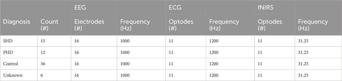
TABLE 1. Dataset signal collection information. Several other signal types were available with the dataset but were omitted due to a lack of relevance to HD. The six “Unknown” patients could not be classified due to health issues.

The data acquisition protocol was conducted as follows. The subjects were seated in a chair with their eyes open and shown/played no visual or audio stimuli. Over the course of a 30 min window, EEG, ECG, and fNIRS were simultaneously recorded. The EEG signal was acquired via a 16-electrode system at a 1-kHz sampling rate through a Brain Products V-Amp system. The ECG was recorded via electrodes placed on each shoulder and on the lower rib at a 1.2 kHz sampling rate. The fNIRS signal was collected at a 31.25 Hz sampling rate over an NIRx NIRScout LED system with 11 optodes. In post-processing, the 30 min samples were all cut down to 20 min.

The EEG and fNIRS sensors were placed according to the standard 10–20 system. Each of the 16 electrodes used for EEG—locations C3, C4, Cz, F3, F4, Fp1, Fp2, O1, O2, P3, P4, P7, P8, Pz, T7, and T8 on the 10–20 system—was mapped to its own channel: 16 in total. The three ECG signal sensors were aggregated to a single channel. For fNIRS, each of the 11 optodes—locations N1, N2, N3, N4, N5, N6, N7, N8, N9, N10, and N11—rendered both deoxygenated and oxygenated blood flow data, giving two channels per optode for a total of 22 fNIRS channels.

3.2 Data pre-processing

To be used for classification, the EEG, ECG, and fNIRS signal data had to be preprocessed to prepare them for feature extraction. Figure 1 displays the preprocessing steps taken immediately after signal acquisition: artifact removal via bandpass filtering and segmentation into epochs. All preprocessing was performed via the MNE library (Gramfort et al., 2013).

FIGURE 1

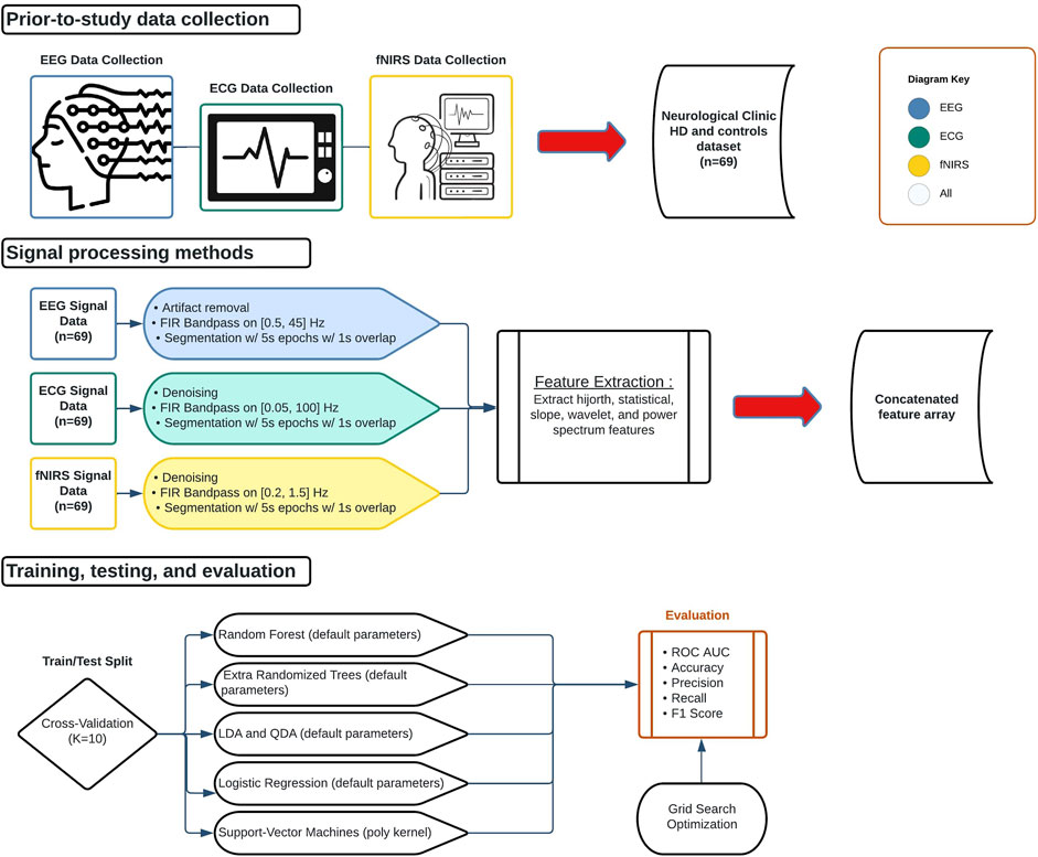
FIGURE 1. Biological signal data applications flowchart. Data collection began outside the scope of the study. Signals were then processed, partitioned, trained, and tested. All signals were processed separately but underwent the same feature extraction procedure and were concatenated into a 1D array for each epoch.

The data were first converted to an MNE object in accordance with the 10–20 standard system for electrode placement to allow us to utilize MNE preprocessing functions. Next, the EEG, ECG, and fNIRS data were filtered via finite impulse response (FIR) bandpass in order to standardize the frequency spectrum across a signal and remove the noise from high and low frequencies. The EEG signal was bandpassed on a domain of [0.5 Hz, 45 Hz] to isolate the delta, theta, and alpha frequency bands, in which abnormalities can be indicative of HD (Ponomareva et al., 2014). The ECG data were filtered on a domain of [0.05 Hz, 100 Hz], where the low pass is the lowest frequency recorded by the machine, and the high pass was to eliminate high-frequency noise (Kher, 2019). The fNIRS signal was filtered on a domain of [0.2 Hz, 1.5 Hz] to remove artifacts caused by blood pressure fluctuations (Klein and Kranczioch, 2019).

The filtered signals for EEG, ECG, and fNIRS were then segmented into 5s epochs with 1s overlap (4s of unique data each) with the goal of increasing training samples and readability (due to high Hz recording). Each patient finally had 1,200s of data for each of EEG, ECG, and fNIRS, and thus the segmentation created 300 epochs per signal per patient. Finally, each data array was normalized by subtracting the mean of the channel for the signal and then packaged in a .npy file.

3.3 Feature extraction procedure

The time and frequency domain features shown in Table 2 were extracted from the processed signals. Figure 2 shows the overall feature extraction procedure, where the extracted time domain and frequency domain features were subsequently concatenated into a single feature array. In terms of specific parameters, a single value for each of the features is calculated for all of the epoch intervals for each patient. The specific bands used for power spectral density and the wavelet functions chosen will be articulated later. Apart from this, there were no particular parameters used other than the formulas themselves.

TABLE 2

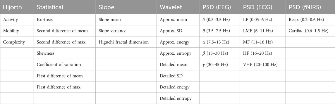
TABLE 2. List of all extracted features. Features were extracted from the time domain signal, the wavelet transformed frequency domain signal, and the Welch-transformed frequency domain signal. In the ECG power spectrum analysis: LF, low frequency; LMF, lower-middle frequency; MF, middle frequency; HF, high frequency; VHF, very-high frequency.

FIGURE 2

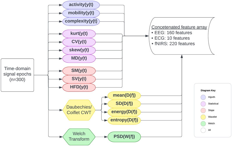
FIGURE 2. Full feature extraction procedure flowchart. The formulas used are detailed elsewhere. Features were extracted for each patient on a per-epoch basis, and for each epoch, a concatenated feature array with the features from all channels and signal types was created.

3.3.1 Time domain features

In signal processing, time domain features can be calculated directly from the raw, time-series data. For the purposes of this study, we chose time domain features to calculate from the list of signal features outlined in Rabha (2016). These include statistical features calculated via mathematical functions of the time series data, Hijorth parameters which measure the signal’s behavior in relation to variance and power, and slope features which, of course, relate to the slope of the signal graph over various intervals.

3.3.1.1 Statistical values

We began by calculating the common statistical values of kurtosis, coefficient of variation, skewness, 1st difference of mean, 2nd difference of mean, 1st difference of max, and 2nd difference of max. A value for each was calculated per channel, per signal, per epoch, and per patient via the following standard formulas applied to the numerical signal data files.

• Kurtosis, calculated via $\mathrm{k}\mathrm{u}\mathrm{r}\mathrm{t}=\frac{{\mu }_4}{{\sigma }^4}$.

• Coefficient of variation, calculated via $\mathrm{C}\mathrm{V}=\frac{\sigma }{\mu }$.

• Skewness, calculated via $\mathrm{s}\mathrm{k}\mathrm{e}\mathrm{w}=\frac{1}{N}{\sum }_{i=1}^N{[\frac{(X_I-\bar{X})}{\sigma }]}^3$.

• 1st and 2nd difference of mean/max, calculated via MD = M_E − M_C.

3.3.1.2 Hijorth parameters

We then calculated the Hijorth parameters of activity, mobility, and complexity because of its success in mental task discrimination in Vourkas et al. (2000). Activity represents the variance or power of the signal over a certain epoch/segment in time domain and is indicative of the power spectrum surface over the frequency domain. Activity can be calculated for a signal sample using the Eq. 1, where y(t) represents the signal function in an epoch.

$\mathrm{a}\mathrm{c}\mathrm{t}\mathrm{i}\mathrm{v}\mathrm{i}\mathrm{t}\mathrm{y}=\mathrm{v}\mathrm{a}\mathrm{r}(\mathrm{y}(\mathrm{t})).(1)$

Mobility indicates the mean frequency over an epoch in the time domain, also represented as the proportion of the standard deviation (SD) over the power spectrum, calculated by manipulating the output from Hijorth’s activity with Eq. 2:

$\mathrm{m}\mathrm{o}\mathrm{b}\mathrm{i}\mathrm{l}\mathrm{i}\mathrm{t}\mathrm{y}=\sqrt{\frac{\mathrm{v}\mathrm{a}\mathrm{r}\left(\frac{\mathrm{d}\mathrm{y}(\mathrm{t})}{\mathrm{d}\mathrm{t}}\right)}{\mathrm{A}\mathrm{c}\mathrm{t}\mathrm{i}\mathrm{v}\mathrm{i}\mathrm{t}\mathrm{y}(\mathrm{y}(\mathrm{t}))}}.(2)$

Lastly, complexity estimates the bandwidth of the signal over an epoch—essentially, the average power of the second derivative of the signal, calculated by applying functions to Hijorth’s mobility as in Eq. 3:

$\mathrm{c}\mathrm{o}\mathrm{m}\mathrm{p}\mathrm{l}\mathrm{e}\mathrm{x}\mathrm{i}\mathrm{t}\mathrm{y}=\frac{\mathrm{M}\mathrm{o}\mathrm{b}\mathrm{i}\mathrm{l}\mathrm{i}\mathrm{t}\mathrm{y}\left(\frac{\mathrm{d}\mathrm{y}(\mathrm{t})}{\mathrm{d}\mathrm{t}}\right)}{\mathrm{M}\mathrm{o}\mathrm{b}\mathrm{i}\mathrm{l}\mathrm{i}\mathrm{t}\mathrm{y}(\mathrm{y}(\mathrm{t})))}.(3)$

3.3.1.3 Slope features

Finally, we calculated features regarding signal slope. Two simple features were first calculated: slope mean and variance.

• Slope mean, calculated via $\mathrm{S}\mathrm{M}=\frac{{\sum }_{i=1}^N\frac{\text{d}y(t)}{\text{d}t}}{N}.$

• Slope variance, calculated via $\mathrm{S}\mathrm{V}=\frac{{\sigma }^2}{S_{xx}}.$

In addition, the Higuchi fractal dimension (HFD) was calculated due to the information it provides about brain response, demonstrated in Gladun (2020). HFD is calculated via the conceptual method outlined by Higuchi (1988). We specifically used the functions to calculate HFD created by INuritdino (2020).

3.3.2 Frequency domain features

To extract frequency domain features, two transforms were used to extract separate features to convert the time series to the frequency domain: the discrete wavelet transform and the Welch transform.

3.3.2.1 Wavelet features

Wavelet features were calculated using the PyWavelets library (Lee et al., 2019). In order to ensure consistency within the dataset and thus enable optimal training, we chose a wavelet function on a per-signal basis and kept the wavelet function the same across epochs and patients. The wavelet function used was chosen by observing samples of the normalized signals, shown in Figure 5. For the preprocessed EEG and fNIRS data, a Coiflet (coif1) discrete wavelet transform was performed on each sample. For ECG, the Daubechies (db4) discrete wavelet transform was utilized. The coefficients that resulted from these transforms were stored in a .txt file. The approximate mean, detailed mean, standard deviation, energy, and entropy were then calculated from these coefficients for each sample. Energy is the summation of the squared signal, calculated by Eq. 4, where C is a coefficient:

$\mathrm{e}\mathrm{n}\mathrm{e}\mathrm{r}\mathrm{g}{\mathrm{y}}_{\mathrm{s}}={\displaystyle \sum _{i=0}^k}{C}_s^2.(4)$

Entropy is the measure of regularity/fluctuation in a time segment, shown in Eq. 5:

$\mathrm{e}\mathrm{n}\mathrm{t}\mathrm{r}\mathrm{o}\mathrm{p}{\mathrm{y}}_{\mathrm{s}}=\log C_s^2\cdot {\displaystyle \sum _{i=0}^k}{C}_s^2.(5)$

3.3.2.2 Power spectral density

Power spectral density (PSD) indicates the power levels over the frequency domain in each component of a signal segment, informing the model of the range of power. This makes it an effective predictor of abnormalities (Boonyakitanont et al., 2020).

Due to the success of EEG PSD for HD diagnosis in Odish et al. (2018), similar PSD bounds for EEG were used in this work. The bounds for ECG PSD bands were chosen based on the peak powers of typical ECG signals, as calculated in McNames et al. (2002): low [0.05 Hz, 6 Hz], low-medium [6 Hz, 11 Hz], medium [11 Hz, 16 Hz], high [16 Hz, 20 Hz], and very high [20 Hz, 100 Hz]. The bounds for fNIRS were chosen based on respiration and heartbeat frequencies from Rahman et al. (2019): respiration [0.2, 0.6 Hz] and cardiac [0.6 Hz, 1.5 Hz].

Welch’s method of calculating PSD is an alternative approximation to the fast Fourier transform (FFT), represented through the equation in Smith (2011). Welch’s method slices the original signal and averages their spectral periodograms, producing a cleaner output than from FFT. In our case, PSD was calculated via built-in MNE functions as shown below in Eq. 6.

$\mathrm{P}\mathrm{S}{\mathrm{D}}^{{}_{\mathrm{x}}^{\mathrm{Welch}}}{\left({\omega }_k\right)}_{=}^{\mathrm{\Delta }}\frac{1}{K}{\displaystyle \sum _{m=0}^{K-1}}{P}_{x_m},\mathrm{M}({\omega }_{\text{k}}).(6)$

The final concatenated data array was calculated from 300 time-epochs per channel per signal (EEG, ECG, or fNIRS) per patient. The final concatenated data array included statistical, Hijorth, slope, wavelet, and PSD features for each channel per signal per epoch per patient, amounting to 948 feature values for each of 300 epochs for each of 69 patients (20,700 epochs total).

3.4 Model selection

Classical machine learning algorithms were used to bin each of the 20,700 concatenated feature epochs as HD-positive or HD-negative. We began by reviewing all classification models offered by the Scikit-learn library (Pedregosa et al., 2011). We utilized common shallow machine learning models that typically perform well on signal features (Shoeibi et al., 2021), as well as discriminant models due to their success in Alzheimer’s EEG analysis.

• Random forest is an ensemble method that uses many randomized decision trees, each of which are trained/fitted on sub-samples of the dataset and subsets of the features at each split point, with their results averaged. This robust approach of different features at each tree split point has been shown to improve accuracy, reduce variability, and reduce overfitting. The specific classification parameters used were Gini impurity loss, “sqrt” max features, no limit on max depth, and an estimator count of either 100 or 1000.

• Extremely randomized trees (ERTs) are an ensemble method in and of themselves; they are similar to random forest in that ERTs take subsets of the features to train each sub-tree but are unlike it in that ERTs train each sub-tree on the entire dataset instead of a sub-sample. ERTs can also select either a random or the best split for the optimal split, unlike the greedy algorithm of random forest. Apart from the estimator count being set to either 100 or 1,000, all other parameters were kept as the Scikit-learn default.

• Logistical regression is effectively a linear regressor that models the data using a sigmoid function instead of a linear function. The algorithm itself remains similar to a linear regressor until the decision threshold, whereas, in binomial logistical regression, the probabilistic result is reduced to a binary output. Apart from using L2 penalty with intercept fitting, all other parameters kept the default.

• Support vector machines (SVMs) use hyper planes to effectively partition data into classes and are thus better suited for classification rather than regression. Based on the number of features, the algorithm found, in an N-dimensional plane, an equation of N-1 dimensions that partitions the data into various classes—in this case two classes (0 or 1)—by minimizing the distance between the equation graph and the individual data points (functional margin). Preliminary tests showed that a parameter configuration with polynomial kernel, scale gamma, and mid-tolerance led to optimal results, and were thus used.

• Linear discriminant analysis (LDA) uses a similar method to SVM, attempting to draw planes to divide sets of classes in the hyperplane of features, but using different criteria. LDA attempts to maximize the mean distance between the points and the hyperplane and minimize the variance between each class. Apart from using the singular value decomposition algorithm for the solution, all other parameters were kept as default.

• Quadratic discriminant analysis (QDA) uses the same criteria as LDA but with a degree-2 discriminant plane rather than linear. All parameters were kept as default.

3.5 Testing procedure

The patients classified as unknown were considered control patients to avoid interfering with training. The classification was performed with each of the above machine learning algorithms on the concatenated feature array, which includes all the time-domain and frequency-domain features for all three signals. The metrics of accuracy, precision, recall, f1 score, and receiver operator characteristic area under the curve (ROC AUC) are recorded over three separate runs and then averaged to ensure accurate results.

For the validation technique, the models were evaluated with 10-fold cross validation (10:1 partitioning ratio). The folds were stratified, meaning that the distribution of controls to HD patients was kept the same as the ratio in the original dataset, leading to more legitimate training. Data were split on folds in accordance with a group array that specified which epochs belonged to which patient, preventing different epochs of the same patient from being placed in both the training and testing sets—which would cause overfitting. Instead, the entirety of any given patient’s epochs would be placed in either the training or the testing set.

4 Results

4.1 Model results

The models outlined were first run with default hyperparameters that tested a variety of metrics on a personal computer with an Intel Core i7-3930k CPU and NVIDIA GeForce RTX-2060 GPU. The concatenated feature vectors were created along with the label and group arrays and were fed into cross-validation. The results of the models are shown in Table 3. As can be seen, the ERT performed best, with random forest close behind on all metrics except recall and f1 score, where the random forest respectively outperformed and tied with the ERT. Plots were created for the ERT and random forest models (estimators = 1000) from the AUC of the receiver operating characteristic, as well as the AUC from the precision and recall for the precision–recall curve (Figure 3).

TABLE 3

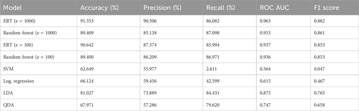
TABLE 3. Results for binary classification with all models using default hyperparameters. Tested with k = 10 with a group array with all epochs of all patients (n = 20,700). Metrics were calculated from sci-kit functions from saved prediction thresholds. “cross_val_predict” was used.

FIGURE 3

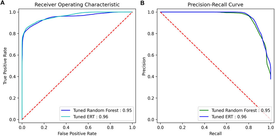
FIGURE 3. ROC AUC and precision–recall AUC for random forest and ERT (estimators = 1000). (A) ROC curve, (B) precision–recall curve.

4.2 Validation

4.2.1 Statistical analysis

To further analyze the results, statistical analysis between the independent variables (the features extracted from the signal data) and the dependent variable (binary HD positivity) was conducted using Statsmodels (Seabold and Perktold, 2010).

Between the entire feature array and the ground truth results, the R² coefficient of determination—representing the proportion of variation of the dependent variable (diagnosis result) explainable by the independent variable (extracted features)—was calculated to be 0.89 or 89%.

The probability-F-statistic was calculated to be 0, representing the probability that the observed correlation between the extracted features and HD positivity occurred by chance. Effectively, this probability approaches 0%.

Statistical significance was also calculated on a per-feature basis, where each feature calculated from each channel was treated as a separate point. It was observed that 577 out of the 948 total features had p < 0.05, with 357 of them having p-values close or equal to zero. The complete list of feature counts across various intervals of p is shown in Table 4.

TABLE 4

TABLE 4. Variety of statistical significance values for various p-value thresholds on a feature-by-feature basis (n = 948). Statistical significance was calculated independent of any prediction model, with a p-value for each feature.

4.2.2 The “black box” problem

The nature of shallow machine learning combined with a large number of features, as in this study, makes it difficult to directly explain the model’s logic. Feature importance can thus be used to at least specify which features the model utilized most for decision making. As Gini impurity was used with random forest, feature importance was calculated via a mean decrease in impurity. The feature array was split up on the basis of various attributes, such as the general group of feature, the type of signal, the specific channels, and the bands, with feature importance calculated on each. Each importance is shown in Figure 4.

FIGURE 4

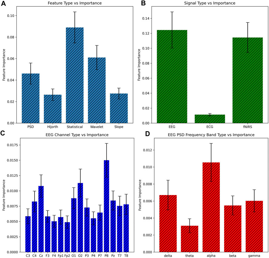
FIGURE 4. Comparison of feature importance ± 1 SE based on various subsets of features. Feature importance was calculated based on the mean decrease in impurity, and all features of a certain subset were added together for the bar graph. (A) Basis of feature, (B) basis of signal, (C) basis of EEG channel, and (D) basis of the EEG PSD band.

5 Discussion

In this study, the aggregation of a number of time-domain and frequency-domain features from EEG, ECG, and fNIRS demonstrated promising predictive power in differentiating both presymptomatic HD patients and symptomatic HD patients from controls. It is safe to conclude that the random forest and ERT tree-based algorithms perform best on large numbers of features such as used here. The hierarchical structure and ability to build connections between trees seemed to allow the ERT and random forest approaches to train with more multivariates. Nevertheless, it is interesting that increasing the number of estimators tenfold led to only a small improvement in the metrics, perhaps because the given number of estimators was sufficient to build enough connections to correlate signal abnormalities to HD positivity.

While providing a full explanation of the procedure we outline is difficult, we do attempt to reveal some insights via statistical analysis. The statistics show that about 11% of the variance of the HD diagnosis result was inexplicable by variance in the independent feature variables, indicating that there could be other signal types of features that could lend more predictive power to the independent variables.

Additionally, the feature importance observations provide insights into the values most indicative of HD. The prime importance of the EEG signal is to be expected since the effects of HD principally inhibit intracellular communication via neurodegeneration, which the signal captures in differences in electrical transfer behavior. This reduction in electrical activity can even be observed in Figure 5. The lack of ECG significance was somewhat disappointing but was also to be expected for two reasons. The first was the existence of presymptomatic patients, who had only experienced mild neural differences, let alone carryover effects, in the rest of the body. Second, the electrical activity of the heart varies in baseline significantly more from patient-to-patient than the brain, and 69 patients were likely not enough to cancel this effect.

FIGURE 5

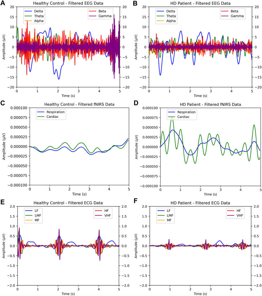
FIGURE 5. Side-by-side comparison of single-epoch samples of EEG, ECG, and fNIRS HD-positive patients versus control patients. As shown, visual discrepancies can be observed between the healthy patient and HD-afflicted patient: the wider amplitude in EEG and ECG, and the closer behavior of respiration and cardiac bands in fNIRS. In (A) and (B), EEG samples for healthy and HD-positive patients are shown. In (C)—(F), the same two patients’ fNIRS and ECG samples are shown.

In terms of feature type, the statistical and wavelet features were the most significant. Since the statistical values encode the most information about signal fluctuation and other surface-level behavior, it seems reasonable that statistical features should be the most important. The wavelet feature importance is more interesting and does suggest that the degree to which a biomedical signal aligns with a pre-chosen waveform helps expose irregular patterns. Another interesting observation is that the P8 channel type was the most significant while the P7 channel was one of low importance, despite both electrodes being attached to directly opposite sides of the head; this was likely due to the asymmetry of the human brain. Each feature importance in the EEG PSD frequency bands was mostly as expected, except for the apparent insignificance of the theta band. Since the theta band is sandwiched between the significant delta and alpha, its poor significance suggests that the theta band recording could have included more noise—our results here thus do not match those of the previous literature.

As outlined previously, computational analysis of biomedical signals for HD is extremely limited. Of these, papers that attempt to directly and computationally diagnose HD with signals used in this paper are limited to two: Odish et al. (2018) and de Tommaso et al. (2003). In Table 5, a comparison with these competing methodologies is shown. Overall, the following advancements/contributions are made over the SOTA by this model:

1. Highest accuracy achieved at 91% and highest ROC AUC at 0.96.

2. Largest dataset with 69 patients, including presymptomatic HD patients.

3. Most signals, feature types, and machine learning models benchmarked.

4. New insights into the types of features most relevant to HD diagnosis and hypotheses as to why.

TABLE 5

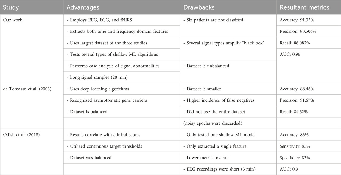
TABLE 5. Summary of advantages, drawbacks, and results of various studies with competing methodologies on the biomedical signal use for HD prognosis.

However, there are noteworthy limitations that arise out of the increased complexity of this procedure as well as the non-streamlined experimental design.

1. The large number of features makes it difficult to pinpoint deeper information into the state of HD progression beyond the diagnosis itself.

2. The long procedure calls for a system that better integrates the process.

3. There is no guarantee that the parameters used for feature extraction and classification are at the highest level of optimization.

4. The use of three signals is a little more expensive, emphasizing the need for preventative care.

In terms of future direction, a few steps can be proposed. First, researchers could attempt to build more controlled algorithms that capture observed trends in the signal data, thus solving the issue of explainability. Second, in order to further improve accuracy and build a more robust model, researchers could make use of data fusion techniques to diversify the pool of training data, much like Khare et al. (2023), and even utilize random grid searching over long run times to find optimal parameters. Third, researchers could look into implementing an integrated deep learning model to more consistently classify patients based on more advanced training. This has already been demonstrated in EfficientNet’s use in classifying PPG signals for cardiac health (El-Dahshan et al., 2024). It would even be possible to improve the usability and preventatives of our proposed solution via an implementation in wearable technology.

Data availability statement

The original contributions presented in the study are included in the article/Supplementary Material; further inquiries can be directed to the corresponding author.

Ethics statement

The studies involving humans were approved by the Commission of the Republic of Slovenia for Medical Ethics. The studies were conducted in accordance with local legislation and institutional requirements. Written informed consent for participation was not required from the participants or their legal guardians/next of kin in accordance with national legislation and institutional requirements.

Author contributions

SM: conceptualization, formal analysis, investigation, methodology, software, validation, visualization, writing–original draft, and writing–review and editing.

Funding

The author declares that no financial support was received for the research, authorship, and/or publication of this article.

Acknowledgments

The author would like to thank Christine Yoon for her mentorship and support throughout this project, including in assisting in the iterative process of editing the manuscript for submission.

Conflict of interest

The author declares that the research was conducted in the absence of any commercial or financial relationships that could be construed as a potential conflict of interest.

Publisher’s note

All claims expressed in this article are solely those of the authors and do not necessarily represent those of their affiliated organizations, or those of the publisher, the editors, and the reviewers. Any product that may be evaluated in this article, or claim that may be made by its manufacturer, is not guaranteed or endorsed by the publisher.

References

Ajitkumar, A., and De Jesus, O. (2022). Huntington disease.

Google Scholar

Bhachawat, S., Shriram, E., Srinivasan, K., and Hu, Y.-C. (2023). Leveraging computational intelligence techniques for diagnosing degenerative nerve diseases: a comprehensive review, open challenges, and future research directions. Diagnostics 13, 288. doi:10.3390/diagnostics13020288

PubMed Abstract | CrossRef Full Text | Google Scholar

Bjerkan, J., Stefanovska, A., Lancaster, G., Kobal, J., and Maglic, B. (2021). Huntington’s disease and controls dataset. Lancaster University Research Directory. doi:10.17635/lancaster/researchdata/416

CrossRef Full Text | Google Scholar

Boonyakitanont, P., Lek-uthai, A., Chomtho, K., and Songsiri, J. (2020). A review of feature extraction and performance evaluation in epileptic seizure detection using eeg. Biomed. Signal Process. Control 57, 101702. doi:10.1016/j.bspc.2019.101702

CrossRef Full Text | Google Scholar

Cassani, R., Falk, T. H., Fraga, F. J., Cecchi, M., Moore, D. K., and Anghinah, R. (2017). Towards automated electroencephalography-based alzheimer’s disease diagnosis using portable low-density devices. Biomed. Signal Process. Control 33, 261–271. doi:10.1016/j.bspc.2016.12.009

CrossRef Full Text | Google Scholar

Chen, J. J., Salat, D. H., and Rosas, H. D. (2012). Complex relationships between cerebral blood flow and brain atrophy in early huntington’s disease. NeuroImage 59, 1043–1051. doi:10.1016/j.neuroimage.2011.08.112

PubMed Abstract | CrossRef Full Text | Google Scholar

Cheng, J., Liu, H.-P., Lin, W.-Y., and Tsai, F.-J. (2020). Identification of contributing genes of huntington’s disease by machine learning. BMC Med. Genomics 13, 176. doi:10.1186/s12920-020-00822-w

PubMed Abstract | CrossRef Full Text | Google Scholar

Colloby, S. J., Cromarty, R. A., Peraza, L. R., Johnsen, K., Jóhannesson, G., Bonanni, L., et al. (2016). Multimodal eeg-mri in the differential diagnosis of alzheimer’s disease and dementia with lewy bodies. J. Psychiatric Res. 78, 48–55. doi:10.1016/j.jpsychires.2016.03.010

CrossRef Full Text | Google Scholar

Dauwan, M., van der Zande, J. J., van Dellen, E., Sommer, I. E., Scheltens, P., Lemstra, A. W., et al. (2016). Random forest to differentiate dementia with lewy bodies from alzheimer’s disease. Alzheimer’s Dementia Diagnosis, Assess. Dis. Monit. 4, 99–106. doi:10.1016/j.dadm.2016.07.003

PubMed Abstract | CrossRef Full Text | Google Scholar

Delussi, M., Nazzaro, V., Ricci, K., and de Tommaso, M. (2020). Eeg functional connectivity and cognitive variables in premanifest and manifest huntington’s disease: eeg low-resolution brain electromagnetic tomography (loreta) study. Front. Physiology 11, 612325. doi:10.3389/fphys.2020.612325

CrossRef Full Text | Google Scholar

de Tommaso, M., De Carlo, F., Difruscolo, O., Massafra, R., Sciruicchio, V., and Bellotti, R. (2003). Detection of subclinical brain electrical activity changes in huntington’s disease using artificial neural networks. Clin. Neurophysiol. 114, 1237–1245. doi:10.1016/S1388-2457(03)00074-9

PubMed Abstract | CrossRef Full Text | Google Scholar

Durongbhan, P., Zhao, Y., Chen, L., Zis, P., De Marco, M., Unwin, Z. C., et al. (2019). A dementia classification framework using frequency and time-frequency features based on eeg signals. IEEE Trans. Neural Syst. Rehabilitation Eng. 27, 826–835. doi:10.1109/TNSRE.2019.2909100

CrossRef Full Text | Google Scholar

Eirola, E., Akusok, A., Björk, K.-M., Johnson, H., and Lendasse, A. (2018). “Predicting huntington’s disease: extreme learning machine with missing values,” in Proceedings of ELM-2016. Editors J. Cao, E. Cambria, A. Lendasse, Y. Miche, and C. M. Vong (Cham: Springer International Publishing), 195–206.

CrossRef Full Text | Google Scholar

El-Dahshan, E.-S. A., Bassiouni, M. M., Khare, S. K., Tan, R.-S., and Rajendra Acharya, U. (2024). Exhyptnet: an explainable diagnosis of hypertension using efficientnet with ppg signals. Expert Syst. Appl. 239, 122388. doi:10.1016/j.eswa.2023.122388

CrossRef Full Text | Google Scholar

fNIRS Lab, C. H. (2018). Functional near-infrared spectroscopy (fnirs)

Google Scholar

Ganesh, S., Chithambaram, T., Krishnan, N. R., Vincent, D. R., Kaliappan, J., and Srinivasan, K. (2023). Exploring huntington’s disease diagnosis via artificial intelligence models: a comprehensive review. Diagnostics 13, 3592. doi:10.3390/diagnostics13233592

PubMed Abstract | CrossRef Full Text | Google Scholar

Gladun, K. (2020). Higuchi fractal dimension as a method for assessing response to sound stimuli in patients with diffuse axonal brain injury. Sovrem. Tehnol. V. Med. 12, 63. doi:10.17691/stm2020.12.4.08

CrossRef Full Text | Google Scholar

Gramfort, A., Luessi, M., Larson, E., Engemann, D. A., Strohmeier, D., Brodbeck, C., et al. (2013). MEG and EEG data analysis with MNE-Python. Front. Neurosci. 7, 267. doi:10.3389/fnins.2013.00267

PubMed Abstract | CrossRef Full Text | Google Scholar

Higuchi, T. (1988). Approach to an irregular time series on the basis of the fractal theory. Phys. D. Nonlinear Phenom. 31, 277–283. doi:10.1016/0167-2789(88)90081-4

CrossRef Full Text | Google Scholar

INuritdino (2020). Higuchi fractal dimension (hfd). Available at: https://github.com/inuritdino/HiguchiFractalDimension.

Google Scholar

Jeong, D.-H., Kim, Y.-D., Song, I.-U., Chung, Y.-A., and Jeong, J. (2016). Wavelet energy and wavelet coherence as eeg biomarkers for the diagnosis of Parkinson’s disease-related dementia and alzheimer’s disease. Entropy 18, 8. doi:10.3390/e18010008

CrossRef Full Text | Google Scholar

Khare, S. K., March, S., Barua, P. D., Gadre, V. M., and Acharya, U. R. (2023). Application of data fusion for automated detection of children with developmental and mental disorders: a systematic review of the last decade. Inf. Fusion 99, 101898. doi:10.1016/j.inffus.2023.101898

CrossRef Full Text | Google Scholar

Kher, R. (2019). Signal processing techniques for removing noise from ecg signals

Google Scholar

Klein, F., and Kranczioch, C. (2019). Signal processing in fnirs: a case for the removal of systemic activity for single trial data. Front. Hum. Neurosci. 13, 331. doi:10.3389/fnhum.2019.00331

PubMed Abstract | CrossRef Full Text | Google Scholar

Kugler, P., Jaremenko, C., Schlachetzki, J., Winkler, J., Klucken, J., and Eskofier, B. (2013). “Automatic recognition of Parkinson’s disease using surface electromyography during standardized gait tests,” in 2013 35th Annual International Conference of the IEEE Engineering in Medicine and Biology Society (IEEE), 5781–5784. doi:10.1109/EMBC.2013.6610865

PubMed Abstract | CrossRef Full Text | Google Scholar

Kulkarni, N., and Bairagi, V. (2014). Diagnosis of alzheimer disease using eeg signals. Int. J. Eng. Res. Technol. doi:10.17577/IJERTV3IS041875

CrossRef Full Text | Google Scholar

Lee, G. R., Gommers, R., Waselewski, F., Wohlfahrt, K., and Leary, A. (2019). Pywavelets: a python package for wavelet analysis. J. Open Source Softw. 4, 1237. doi:10.21105/joss.01237

CrossRef Full Text | Google Scholar

Mason, S. L., Daws, R. E., Soreq, E., Johnson, E. B., Scahill, R. I., Tabrizi, S. J., et al. (2018). Predicting clinical diagnosis in huntington’s disease: an imaging polymarker. Ann. Neurology 83, 532–543. doi:10.1002/ana.25171

PubMed Abstract | CrossRef Full Text | Google Scholar

McBride, J. C., Zhao, X., Munro, N. B., Jicha, G. A., Schmitt, F. A., Kryscio, R. J., et al. (2015). Sugihara causality analysis of scalp eeg for detection of early alzheimer’s disease. NeuroImage Clin. 7, 258–265. doi:10.1016/j.nicl.2014.12.005

PubMed Abstract | CrossRef Full Text | Google Scholar

McColgan, P., and Tabrizi, S. (2018). Huntington’s disease: a clinical review. Eur. J. Neurology 25, 24–34. doi:10.1111/ene.13413

CrossRef Full Text | Google Scholar

McNames, J., Crespo, C., Aboy, M., Bassale, J., Jenkins, L., and Goldstein, B. (2002). “Harmonic spectrogram for the analysis of semi-periodic physiologic signals,” in Proceedings of the Second Joint 24th Annual Conference and the Annual Fall Meeting of the Biomedical Engineering Society] [Engineering in Medicine and Biology. doi:10.1109/IEMBS.2002.1134427

CrossRef Full Text | Google Scholar

Mohan, A., Sun, Z., Ghosh, S., Li, Y., Sathe, S., Hu, J., et al. (2022). A machine-learning derived huntington’s disease progression model: insights for clinical trial design. Mov. Disord. 37, 553–562. doi:10.1002/mds.28866

PubMed Abstract | CrossRef Full Text | Google Scholar

Nguyen, L., Bradshaw, J. L., Stout, J. C., Croft, R. J., and Georgiou-Karistianis, N. (2010). Electrophysiological measures as potential biomarkers in huntington’s disease: review and future directions. Brain Res. Rev. 64, 177–194. doi:10.1016/j.brainresrev.2010.03.004

PubMed Abstract | CrossRef Full Text | Google Scholar

Nikas, J. B., and Low, W. C. (2011). Application of clustering analyses to the diagnosis of huntington disease in mice and other diseases with well-defined group boundaries. Comput. Methods Programs Biomed. 104, e133–e147. doi:10.1016/j.cmpb.2011.03.004

PubMed Abstract | CrossRef Full Text | Google Scholar

Novotný, M., Pospisil, J., Cmejla, R., and Rusz, J. (2015). Automatic detection of voice onset time in dysarthric speech, 4340–4344. doi:10.1109/ICASSP.2015.7178790

CrossRef Full Text | Google Scholar

Odish, O., Johnsen, K., Someren, P., Roos, R., and Dijk, J. G. v. (2018). Eeg may serve as a biomarker in huntington’s disease using machine learning automatic classification. Sci. Rep. 8, 16090. doi:10.1038/s41598-018-34269-y

PubMed Abstract | CrossRef Full Text | Google Scholar

Oguz, I. (2011). Early detection of huntington’s disease: longitudinal analysis of basal ganglia and cortical thickness. Vanderbilt Institute for Surgery and Engineering. Project Number: 5R01NS094456-05.

Google Scholar

Paulsen, J., Langbehn, D., Stout, J., Aylward, E., Ross, C., Nance, M., et al. (2008). Detection of huntington’s disease decades before diagnosis: the predict-hd study. JNNP. doi:10.1136/jnnp.2007.128728

CrossRef Full Text | Google Scholar

Pedregosa, F., Varoquaux, G., Gramfort, A., Michel, V., Thirion, B., Grisel, O., et al. (2011). Scikit-learn: machine learning in Python. J. Mach. Learn. Res. doi:10.5555/1953048.2078195

CrossRef Full Text | Google Scholar

Ponomareva, N., Klyushnikov, S., Abramyacheva, N., Malina, D., Scheglova, N., Fokin, V., et al. (2014). Alpha-theta border eeg abnormalities in preclinical huntington’s disease. J. Neurological Sci. 344, 114–120. doi:10.1016/j.jns.2014.06.035

PubMed Abstract | CrossRef Full Text | Google Scholar

Ponomareva, N. V., Klyushnikov, S. A., Abramycheva, N., Konovalov, R. N., Krotenkova, M., Kolesnikova, E., et al. (2023). Neurophysiological hallmarks of huntington’s disease progression: an eeg and fmri connectivity study. Front. Aging Neurosci. 15, 1270226. doi:10.3389/fnagi.2023.1270226

PubMed Abstract | CrossRef Full Text | Google Scholar

Rabha, J. (2016). Feature extraction of mental load eeg signals. Available at: https://github.com/JoyRabha/Feature-Extraction-EEG.

Google Scholar

Rahman, M. A., Rashid, M. A., and Ahmad, M. (2019). Selecting the optimal conditions of savitzky–golay filter for fnirs signal. Biocybern. Biomed. Eng. 39, 624–637. doi:10.1016/j.bbe.2019.06.004

CrossRef Full Text | Google Scholar

Ramzan, F., Khan, M. U. G., Rehmat, A., Iqbal, S., Saba, T., Rehman, A., et al. (2019). A deep learning approach for automated diagnosis and multi-class classification of alzheimer’s disease stages using resting-state fmri and residual neural networks. J. Med. Syst. 44, 37. doi:10.1007/s10916-019-1475-2

PubMed Abstract | CrossRef Full Text | Google Scholar

Rizk-Jackson, A., Stoffers, D., Sheldon, S., Kuperman, J., Dale, A., Goldstein, J., et al. (2011). Evaluating imaging biomarkers for neurodegeneration in pre-symptomatic huntington’s disease using machine learning techniques. NeuroImage 56, 788–796. doi:10.1016/j.neuroimage.2010.04.273

PubMed Abstract | CrossRef Full Text | Google Scholar

Rossini, P., Di Iorio, R., Vecchio, F., Anfossi, M., Babiloni, C., Bozzali, M., et al. (2020). Early diagnosis of alzheimer’s disease: the role of biomarkers including advanced eeg signal analysis. report from the ifcn-sponsored panel of experts. Clin. Neurophysiol. 131, 1287–1310. doi:10.1016/j.clinph.2020.03.003

PubMed Abstract | CrossRef Full Text | Google Scholar

Schneider, S. A., and Bird, T. (2016). Huntington’s disease, huntington’s disease look-alikes, and benign hereditary chorea: what’s new? Mov. Disord. Clin. Pract. 3, 342–354. doi:10.1002/mdc3.12312

PubMed Abstract | CrossRef Full Text | Google Scholar

Seabold, S., and Perktold, J. (2010). “Statsmodels: econometric and statistical modeling with Python,” in Proceedings of the 9th Python in Science Conference. doi:10.25080/Majora-92bf1922-011

CrossRef Full Text | Google Scholar

Shoeibi, A., Sadeghi, D., Moridian, P., Ghassemi, N., Heras, J., Alizadehsani, R., et al. (2021). Automatic diagnosis of schizophrenia in eeg signals using cnn-lstm models. Front. Neuroinformatics 15, 777977. doi:10.3389/fninf.2021.777977

CrossRef Full Text | Google Scholar

Smith, J. O. (2011). Spectral audio signal processing. 2011 edition. CCRMA-Stanford University. Online book.

Google Scholar

Stephen, C. D., Hung, J., Schifitto, G., Hersch, S. M., and Rosas, H. D. (2018). Electrocardiogram abnormalities suggest aberrant cardiac conduction in huntington’s disease. Mov. Disord. Clin. Pract. 5, 306–311. doi:10.1002/mdc3.12596

PubMed Abstract | CrossRef Full Text | Google Scholar

Tăuţan, A.-M., Ionescu, B., and Santarnecchi, E. (2021). Artificial intelligence in neurodegenerative diseases: a review of available tools with a focus on machine learning techniques. Artif. Intell. Med. 117, 102081. doi:10.1016/j.artmed.2021.102081

PubMed Abstract | CrossRef Full Text | Google Scholar

Trambaiolli, L., Spolaôr, N., Lorena, A., Anghinah, R., and Sato, J. (2017). Feature selection before eeg classification supports the diagnosis of alzheimer’s disease. Clin. Neurophysiol. 128, 2058–2067. doi:10.1016/j.clinph.2017.06.251

PubMed Abstract | CrossRef Full Text | Google Scholar

Vespa, P. M., Nenov, V., and Nuwer, M. R. (1999). Continuous eeg monitoring in the intensive care unit: early findings and clinical efficacy. J. Clin. Neurophysiology 16, 1–13. doi:10.1097/00004691-199901000-00001

PubMed Abstract | CrossRef Full Text | Google Scholar

Vourkas, M., Micheloyannis, S., and Papadourakis, G. (2000). “Use of ann and hjorth parameters in mental-task discrimination,” in 2000 First International Conference Advances in Medical Signal and Information Processing (IEE Conf. Publ. No. 476), 327–332. doi:10.1049/cp:20000356

CrossRef Full Text | Google Scholar

Zhang, X., Barkhaus, P., Rymer, W., and Zhou, P. (2013). Machine learning for supporting diagnosis of amyotrophic lateral sclerosis using surface electromyogram. IEEE Trans. neural Syst. rehabilitation Eng. 22, 96–103. doi:10.1109/TNSRE.2013.2274658

CrossRef Full Text | Google Scholar

Zhu, Y., Shamblin, I., Rodriguez, E., Salzer, G. E., Araysi, L., Margolies, K. A., et al. (2019). Progressive cardiac arrhythmias and ECG abnormalities in the Huntington’s disease BACHD mouse model. Hum. Mol. Genet. 29, 369–381. doi:10.1093/hmg/ddz295

PubMed Abstract | CrossRef Full Text | Google Scholar