Direction of arrival estimation using the rotating equatorial microphone

1 Introduction

Estimating the direction of arrival (DOA) of acoustic sources conventionally requires a microphone array consisting of at least two microphones. This poses a problem in situations where space is limited and cost must be minimized. Over the years several approaches have been proposed for DOA estimation using only a single microphone, many of which are inspired from theories of human monaural sound localization. These approaches typically place a synthetic pinna or an arbitrarily shaped scattering body with known DOA-dependent scattering characteristics close to a stationary microphone to induce spatial localization cues. Additionally, knowledge of the spectral characteristics of the sound sources to be localized is required, as it is otherwise impossible to differentiate the localization cues from the sound source.

The first implementation of single microphone localization was performed in Harris et al. (2000), where the DOA of an acoustic pulse was determined using a reflector that was designed to produce two echoes, which arrive at the microphone at different DOA-dependent times. This time difference of arrival is subsequently determined using cross-correlation, from which the DOA is inferred. A more elaborate approach was employed in Takiguchi et al. (2009), where a Gaussian mixture model (GMM) was trained on speech to subsequently estimate the acoustic transfer functions between the microphone and a speech source placed at various locations. As the characteristics of the room are used to induce localization cues, this method requires retraining for each room and microphone placement. This was circumvented in Fuchs et al. (2011), where the head-related transfer function (HRTF) of a dummy head was measured and a speech model was trained using a GMM. Using the HRTF data, the GMMs for speech arriving at various DOAs were computed and subsequently used to estimate the DOA of a speech source. A more sophisticated approach was implemented in El Badawy et al. (2017) and their following work El Badawy and Dokmanić (2018), where the directional-dependent scattering of arbitrary LEGO^® constructions was measured and localization of white noise was performed using non-negative matrix factorization. This approach also allowed for the localization of up to two speech sources utilizing non-negative dictionaries trained on speech.

A more general source localization approach was implemented in Saxena and Ng (2009), where a hidden Markov model was trained on common real-world sounds (i.e., human speech, animal noises and nature sounds) and the DOA-dependent transfer functions of multiple scattering bodies were measured. The DOA of various sounds was subsequently estimated by finding the azimuth angle most likely to produce the observed signal.

A different approach was employed in Kim and Kim (2015), where multiple, differently sized pyramidal horns were placed around a microphone, inducing DOA-dependent acoustic resonance. As this resonance introduces a characteristic fingerprint in the spectrum of recorded wideband sound sources, localization is feasible without knowledge of the spectral characteristics of the sources. The downside to this approach is the large required size and low localization resolution due to the dimensions of the pyramidal horns.

Some approaches require a certain movement of either the microphone or a reflecting element. In Takashima et al. (2010) a parabolic reflection board was attached to a microphone and manually rotated to estimate the acoustic transfer function between the microphone and a speech source for different board orientations. Given a GMM speech model, a characteristic difference could be observed in the acoustic transfer function as the reflection board was directed at a speech source. A more sophisticated approach was implemented in Tengan et al. (2021) and Tengan et al. (2023), where a directional microphone was sequentially oriented in multiple directions and DOA estimation was performed by locating the maxima in an estimated power spectral density (PSD) vector. This vector was obtained by solving a group-sparsity constrained optimization problem using a dictionary composed of the known DOA-dependent microphone responses. A very different approach was employed in Bui et al. (2018) and their following work Wang et al. (2023) where localization of amplitude-modulated noise and speech was performed with a dummy head using a regression model trained on features of these signals in the so-called monaural modulation spectrum, as well as features in the head-related modulation transfer function. Head movement was additionally employed to eliminate incorrect DOA estimates. Unlike the previously described approaches, which only estimate the two-dimensional DOA, this method also provides elevation information.

Finally, some approaches utilize continuous microphone movement. In Schasse and Martin (2010) and Schasse et al. (2012) a single signal is constructed from a circular microphone array by circular sampling, i.e., taking the first sample from the first microphone, the second sample from the neighboring microphone and so on in a circular fashion. The resulting signal can be viewed as having been captured by a rapidly rotating microphone, the movement of which introduces DOA-dependent periodic Doppler shifts into captured sound sources. In Schasse et al. (2012) the captured signal is decomposed into multiple subbands and the instantaneous frequency of each subband is estimated for each spectrogram frame. As these frequencies shift in a periodic and DOA-dependent manner, the phases of these shifts are computed for each subband to yield the DOA estimates. This method allowed for two-dimensional DOA estimation of up to 5 simultaneous speech sources. In Hioka et al. (2018) this approach was implemented in practice using a single rotating microphone as opposed to a circular microphone array, albeit only single monochromatic sound sources with a known frequency were used as test signals. The microphone rotated at a maximum speed of approximately 17 rotations per second and DOA estimation was shown to be accurate only for frequencies above 500 Hz.

As it can be observed, DOA estimation using a single continuously moving microphone has not been comprehensively studied, despite the promising results from Schasse et al. (2012) showing that it potentially enables single microphone localization without requiring a scattering body or prior knowledge of the source signals’ spectral characteristics. In fact, only limited research has been conducted on moving microphones as a whole. The few instances of study on moving microphones almost exclusively cover the measurement of room impulse responses either along the microphone trajectory, e.g., Ajdler et al. (2007), Hahn and Spors (2015) and Hahn and Spors (2017), or in a given volume of interest using rapid microphone movement, e.g., Katzberg et al. (2017) and Katzberg et al. (2021). Since these approaches rely on known excitation signals for room impulse response measurement, they cannot be modified to allow for DOA estimation of unknown signals.

To investigate DOA estimation and other sound field analysis applications using a single moving microphone, we developed the Rotating Equatorial Microphone (REM) prototype described in Lawrence et al. (2022), which achieves rotational speeds between 24 and 42 rotations per second. The lower limit is constrained by hardware limitations and the upper limit is set to ensure that distortions due to wind and motor noise are not too large. The validation of the proposed algorithm will be conducted using the REM.

The primary concept of our proposed DOA estimation algorithm is to compensate for the DOA-dependent distortions introduced by the microphone rotation for multiple candidate DOAs. We subsequently find the candidates that contain the least distortion according to two metrics which will be introduced in Section 2. As we will show in simulations and practical experiments, this method allows for the estimation of the azimuth of multiple simultaneous sound sources without prior knowledge of the spectral characteristics of the sources. We will also illustrate how the algorithm can be extended to estimate the colatitude of sound sources. However, verification of colatitude estimation is left for future work.

This article is structured as follows: In Section 2, we will elaborate on the distortions that arise when a circularly rotating microphone is placed in a sound field, as well as the assumptions and simplifications that we employ. Subsequently, in Section 3, we will present two algorithms that compensate for two of the distortions described in Section 2 and use them to formulate a DOA estimation algorithm. In Section 4, we will conduct numerical simulations and practical experiments to verify and evaluate the presented algorithm. Finally, in Section 5, we will draw our conclusions and discuss future work.

2 Theoretical foundations

Multiple DOA-dependent spectral distortions are introduced as the microphone rotates in a circular manner. These will be discussed in this section to enable their compensation in Section 3.

2.1 Problem formulation

The high rotational speed employed by the REM induces significant frequency shifts in recorded audio signals due to the Doppler effect. To find a mathematical expression for this phenomenon, consider the following setup: A circularly moving omnidirectional microphone is placed in a free field with a sound source situated at azimuth φ ∈ [0, 2π) relative to the initial microphone position. The circular motion is situated in the x-y plane and characterized by a rotational radius r and angular velocity ω_rot = 2πf_rot. Moreover, the sound source emits a single frequency f_src and is placed sufficiently far away from the microphone such that the incoming sound waves can be approximated by plane waves with a constant amplitude. This setup is depicted in Figure 1A. If we decompose the circular movement into two components, one parallel and one perpendicular to the incoming sound waves, we find that only the perpendicular component introduces Doppler shifts. Therefore, we discard the parallel component and simplify the circular movement to a non-uniform linear movement along the red line in Figure 1B. The instantaneous velocity v (t, φ) along this red line is obtained by projecting the circular movement onto the red line, resulting in

$v\left(t,\phi \right)=-{\omega }_{\text{rot}}\cdot r\cdot \sin \left({\omega }_{\text{rot}}t-\phi \right)=2\pi r\cdot f_{\text{rot}}\cdot \cos \left(2\pi f_{\text{rot}}t-{\phi }^{\prime }\right),(1)$

where ${\phi }^{\prime }=\phi -\frac{\pi }{2}$ and positive velocity is defined as moving towards and negative velocity as moving away from the plane waves. The reasons we choose the cosine and rotational frequency f_rot as opposed to the sine and angular velocity will become evident in Section 2.2.

FIGURE 1

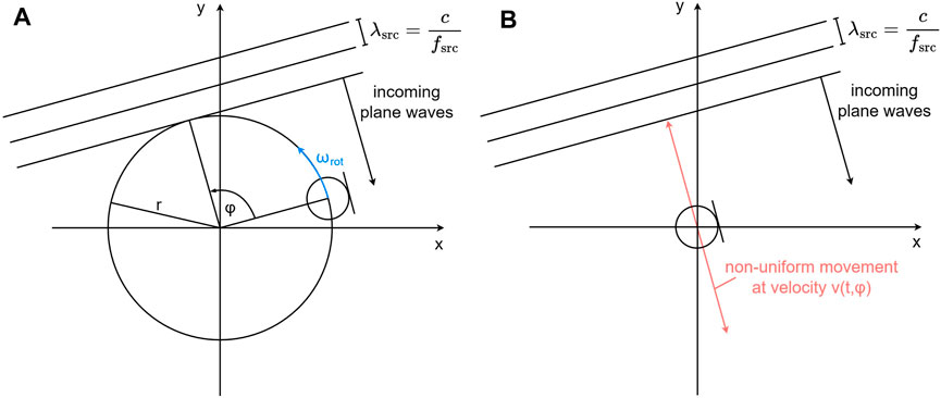
FIGURE 1. Rotating microphone in a two-dimensional sound field composed of plane waves arriving at azimuth φ relative to the initial microphone position. (A) Circular microphone movement. (B) Simplified linear movement

We now extend our considerations to three dimensions, i.e., the plane waves arrive at azimuth φ ∈ [0, 2π) relative to the initial microphone position within the rotational plane and at colatitude θ ∈ [0, π] relative to the rotational plane. The circular motion exhibits the same characteristics as before, as depicted in Figure 2. Once again, we can discard the microphone movement parallel to the incoming sound waves and simplify the microphone movement to an equivalent non-uniform linear movement, which is indicated by the red line. By inserting the purple elements, we can apply basic trigonometry to compute the maximum displacement along the red line relative to the origin as r ⋅ sin(θ). Analogously to Eq. 1, we obtain the instantaneous velocity v (t, φ, θ) of the microphone along the red line by projecting the circular movement onto the red line. This results in

$v\left(t,\phi ,\theta \right)=2\pi r\cdot \sin \left(\theta \right)\cdot f_{\text{rot}}\cdot \cos \left(2\pi f_{\text{rot}}t-{\phi }^{\prime }\right).$

FIGURE 2

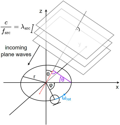
FIGURE 2. Rotating microphone in a three-dimensional sound field composed of plane waves arriving at azimuth φ relative to the initial microphone position and colatitude θ relative to the rotational plane.

Following the well-known definition of the Doppler effect, we can use the previously computed instantaneous velocity to compute the instantaneous frequency observed by the microphone f_obs (t, φ, θ) as

$f_{\text{obs}}\left(t,\phi ,\theta \right)=\left(1+\frac{v\left(t,\phi ,\theta \right)}{c}\right)\cdot f_{\text{src}}=\left(1+\frac{2\pi r\cdot \sin \left(\theta \right)\cdot f_{\text{rot}}\cdot \cos \left(2\pi f_{\text{rot}}t-{\phi }^{\prime }\right)}{c}\right)\cdot f_{\text{src}},(2)$

where c is the speed of sound. The instantaneous phase ϕ_obs (t, φ, θ) is subsequently obtained by integration:

${\varphi }_{\text{obs}}\left(t,\phi ,\theta \right)={\varphi }_{\text{obs}}\left(0,\phi ,\theta \right)+{\int }_0^{t}2\pi f_{\text{obs}}\left(\tau ,\phi ,\theta \right)d\tau =2\pi f_{\text{src}}t+\frac{2\pi r\cdot \sin \left(\theta \right)\cdot f_{\text{src}}}{c}\cdot \sin \left(2\pi f_{\text{rot}}t-{\phi }^{\prime }\right)+{\varphi }_0,$

where ${\varphi }_0={\varphi }_{\text{obs}}(0,\phi ,\theta )+\frac{2\pi r\cdot \sin (\theta )\cdot f_{\text{src}}}{c}\cdot \sin ({\phi }^{\prime })$ is an initial phase offset. We can now express the recorded microphone signal x (t, φ, θ) as

$x\left(t,\phi ,\theta \right)=A_0\cdot \cos \left(\varphi \left(t,\phi ,\theta \right)\right)=A_0\cdot \cos \left(2\pi f_{\text{src}}t+\frac{2\pi r\cdot \sin \left(\theta \right)\cdot f_{\text{src}}}{c}\cdot \sin \left(2\pi f_{\text{rot}}t-{\phi }^{\prime }\right)+{\varphi }_0\right),(3)$

where A₀ is the signal amplitude, which we assume to be unity.

An example spectrogram of $x(t,0,\frac{\pi }{2})$ for f_src = 8 kHz, r = 0.045 m, $c=343\frac{\text{m}}{\text{s}}$, f_rot = 42 Hz, A₀ = 1 and ϕ₀ = 0 is shown in Figure 3A. The spectrogram was computed using a Blackman window, a frame length of L = 512 which has been zero-padded to 8,192, a frame overlap of 97.5% and a sampling rate of f_s = 48 kHz. As it can be observed, the instantaneous frequency fluctuates around the source frequency in a sinusoidal manner. The computation of the phase of this sinusoid allows for the estimation of φ, which is the DOA estimation approach used in Schasse and Martin (2010), Schasse et al. (2012) and Hioka et al. (2018). Moreover, the amplitude of this sinusoid is dependent on θ. Unfortunately, accurate derivation of φ and θ by observing this sinusoid is challenging in practice for wideband and low-frequency signals. This is due to the short required frame length, especially at higher rotational speeds, which results in a low-frequency resolution. Lower rotational speeds are therefore preferred, however, the source signal must also remain sufficiently constant during one rotation to enable accurate amplitude and phase estimation of the sinusoid. Furthermore, lower rotational speeds result in smaller Doppler shifts, further reducing the estimation accuracy. For these reasons, we choose a different approach, which exploits a phenomenon that occurs as we increase the frame length.

FIGURE 3

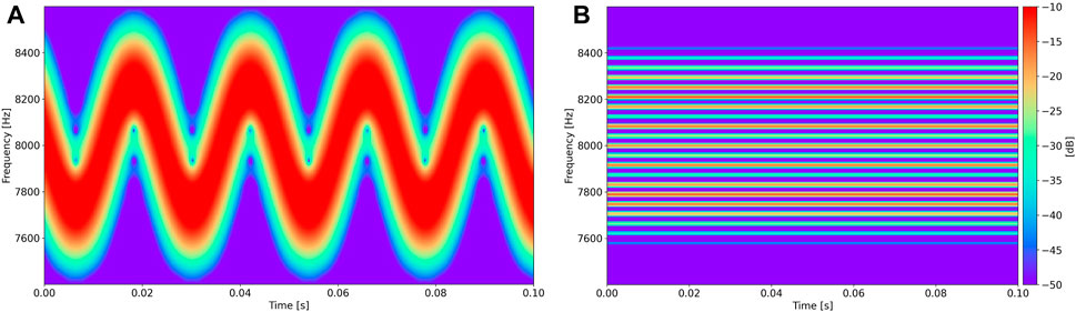
FIGURE 3. Spectrograms of $x(t,0,\frac{\pi }{2})$ for different frame lengths with f_src = 8 kHz, r = 0.045 m, $c=343\frac{\text{m}}{\text{s}}$, f_rot = 42 Hz, A₀ = 1 and ϕ₀ = 0. (A) Frame length L = 512. (B) Frame length L = 8,192.

2.2 Frequency modulation

Figure 3B shows a spectrogram of $x(t,0,\frac{\pi }{2})$ with the same parameters as before, except for the frame length which is now set to L = 8,192. Multiple frequencies can be observed, which are all separated by exactly 42 Hz = f_rot. To explain this phenomenon, note that Eq. 3 resembles a sinusoidal frequency modulated signal x_FM(t), which is commonly used in the field of telecommunications:

$x_{\text{FM}}\left(t\right)=A_c\cdot \cos \left(2\pi f_{c}t+\beta \cdot \sin \left(2\pi f_{m}t\right)\right),(4)$

where f_c is the carrier frequency with amplitude A_c, f_m is the frequency of the modulating wave and β is the so-called modulation index, which quantifies by how much the carrier frequency is modulated. Setting aside phase offsets φ′ and ϕ₀, we can observe that values A₀, f_src and f_rot from Eq. 3 correspond to A_c, f_c and f_m from Eq. 4, respectively. Furthermore, the modulation index shows θ-dependence and corresponds to $\beta (\theta )=\frac{2\pi r\cdot \sin (\theta )\cdot f_{\text{src}}}{c}$. Note that β(θ) is symmetric around $\theta =\frac{\pi }{2}$, indicating that plane waves arriving at $\theta =\frac{\pi }{2}\pm {\theta }^{\prime }$ for ${\theta }^{\prime }\in [0,\frac{\pi }{2}]$ are modulated to the same extent and are therefore not distinguishable from each other. Furthermore, note that the modulation index is independent of the rotational frequency and dependent on the source frequency, i.e., higher frequencies are modulated to a larger extent.

The observation from Figure 3B can now be explained as an alternative representation of sinusoidal frequency-modulated signals, which for Eq. 3 is given by

$\cos \left(2\pi f_{\mathit{src}}t+\beta \left(\theta \right)\cdot \sin \left(2\pi f_{\text{rot}}t-{\phi }^{\prime }\right)+{\varphi }_0\right)={\displaystyle \sum _{n=-\infty }^{\infty }}{J}_n\left(\beta \left(\theta \right)\right)\cdot \cos \left(2\pi \left(f_{\mathit{src}}+n{f}_{\text{rot}}\right)t-n{\phi }^{\prime }+{\varphi }_0\right),$

where J_n (⋅) denotes the Bessel function of the first kind for integer order n. This equation is obtained by following the derivation from Van Der Pol (1930) with the inclusion of initial phase offsets. As it can be observed, a frequency-modulated signal contains infinitely many sidebands spaced at integer multiples of the rotational frequency around the source frequency. Moreover, the modulation index influences the weighting of these sidebands. This is demonstrated in Figure 4A, where the PSDs of frequency modulated 8 kHz sine waves are plotted for an increasing modulation index at frame length L = 8,192.

FIGURE 4

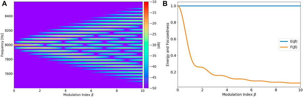
FIGURE 4. Energy and focusedness of an 8 kHz sine wave for an increasing β. The plots in (B) have been normalized by dividing each graph by its maximum value. (A) PSDs of modulated 8 kHz sine waves. (B) Energy and focusedness of (A).

Another noteworthy observation can be made if we estimate the energy of each PSD S_xx(β) from Figure 4A as $E(\beta )={\sum }_{k=0}^{N/2}{S}_{\mathbf{xx}}{(\beta )}_k$, where S_xx(β)_k represents the kth discrete frequency bin of S_xx(β). As Figure 4B shows, the energy stays constant regardless of the modulation index. This is explained by the following property of Bessel functions of the first order:

${\displaystyle \sum _{n=-\infty }^{\infty }}{J}_n^2\left(x\right)=1,\forall x\ge 0,$

as provided by Olver et al., (2023). Sinusoidal frequency modulation can therefore be interpreted as an energy-conserving redistribution of the input energy onto the sidebands. To quantify the degree to which the energy is distributed onto the sidebands, we introduce the following metric:

$F\left(\beta \right)={\displaystyle \sum _{k=0}^{N/2}}{\left(S_{\mathbf{xx}}{\left(\beta \right)}_k\right)}^2.(5)$

We will refer to this metric as focusedness since it becomes larger as the energy is more focused on the source frequency. An example plot of the focusedness is contained in Figure 4B. This metric will be of importance in Section 3.4, where we will compensate for the frequency modulation for multiple candidate DOAs. The frequency modulation present in the resulting compensated signals decreases as the candidate DOAs approach the correct DOA. In other words, the compensated signal associated with the best DOA candidate will feature the highest focusedness.

2.3 Amplitude modulation

Previously, we assumed the microphone to be perfectly omnidirectional. This assumption does not hold in practice, since all microphones feature a direction-dependent non-flat frequency response. Additionally, the apparatus that enables the microphone rotation introduces acoustic scattering, further impacting the effective direction-dependent frequency response of the microphone. These phenomena affect both the amplitude and phase of the captured signal from Eq. 3. In this article, we neglect the influence of the frequency response on the phase and only consider the direction-dependent magnitude response of the microphone.

We will express the direction-dependent magnitude response of the microphone as |H (f_m, φ_m, θ_m)|, where f_m represents the frequency of interest arriving at DOA (φ_m, θ_m) relative to the front of the microphone. The DOA at the front of the microphone is defined as (0, $\frac{\pi }{2}$). The on-axis magnitude response is therefore given by $|H(f_m,0,\frac{\pi }{2})|$. Given knowledge of the direction-dependent magnitude response of the microphone, the DOA-dependent observed amplitude of a sinusoid with frequency f_m and amplitude A₀ can be expressed as A (f_m, φ_m, θ_m) = A₀ ⋅|H (f_m, φ_m, θ_m)|. Considering the setup from Figure 2, we further find that φ_m and θ_m correspond to (φ − 2πf_rot t) mod 2π and θ, respectively. Moreover, f_m corresponds to f_obs (t, φ, θ) from Eq. 2, given by $f_{\text{obs}}(t,\phi ,\theta )=\left(1-\frac{2\pi r\cdot \sin (\theta )\cdot f_{\text{rot}}\cdot \sin (2\pi f_{\text{rot}}t-\phi )}{c}\right)\cdot f_{\text{src}}$.

We can now more accurately represent the amplitude A₀ from Eq. 3 as

$A_0\left(t,f_{\text{src}},\phi ,\theta \right)=A_0\cdot |H\left(\left(1-2\pi r\cdot \sin \left(\theta \right)\cdot f_{\text{rot}}\cdot \sin \left(2\pi f_{\text{rot}}t-\phi \right)/c\right)\cdot f_{\text{src}},\left(\phi -2\pi f_{\text{rot}}t\right)\text{mod}2\pi ,\theta \right)|.(6)$

It can be observed that the amplitude of the signal captured by the microphone is modulated periodically. The period of the modulating wave corresponds to 1/f_rot and its shape is dependent on the microphone’s direction-dependent magnitude response. This periodicity will be exploited in Section 3.4 as follows: Given the direction-dependent magnitude response of our REM prototype, we derive an algorithm that can compensate for the amplitude modulation that is introduced by the microphone rotation for multiple DOA candidates. The compensated signal associated with the best DOA candidate will feature the least amplitude modulation. This signal can be identified by computing the PSD of all compensated signals in a frame-wise manner using a short frame length and shift and finding the signal with the lowest average PSD variance over each rotation period.

2.4 Near field effects, self-induced noise and reverberation

Up until this point we have assumed that the sound field consists of plane waves. In reality, however, sound sources can only be approximated by plane waves in the far field, whereas in the near field the wavefronts will exhibit a non-negligible curvature depending on the geometry of the sound source. This means that in the near field not only the perpendicular but also the parallel component of the microphone movement to the sound waves will introduce Doppler shifts. Additionally, the amplitude A₀ from Eq. 6 will change based on the instantaneous microphone-source distance. It was demonstrated in Duda and Martens (1998) that the acoustic response of a rigid sphere hardly exhibits any distance dependency apart from a scaling of the amplitude if the distance to the sound source is farther than 5 times the sphere radius. In our setup, this factor between source distance and sphere radius is approximately 29. Therefore, we neglect near field effects in this article.

Another significant distortion introduced by the microphone rotation is self-induced noise, also known as ego-noise, due to the mechanical movement of the microphone. The self-induced noise is composed of two primary components: The first component is caused by vibrations due to subtle imbalances of both the motor and the microphone housing. This noise has a harmonic structure with fundamental frequency f_rot. The second component is wind noise, which is caused by the rapid speed of the microphone. Although the friction between the microphone housing and the surrounding air results in airflow around the microphone, causing complex interactions between the airflow and incoming sound waves, we choose to neglect these effects and consider both the wind noise and vibration noise to be independent of recorded source signals. To reduce the self-induced noise we employ spectral subtraction in Section 4 using an estimate of the average noise spectrum directly before each recorded sample. It is worth noting that multiple, more elaborate approaches have been proposed to estimate and reduce self-induced noise, such as those presented in Ince et al. (2011) and Schmidt and Kellermann (2019). For the sake of simplicity, however, we perform noise reduction using spectral subtraction, since noise reduction is not the focus of this article.

The last noteworthy distortion introduced into the recorded signal is caused by acoustic reverberation both within the microphone housing and the room in which the microphone is placed. Although this effect is not specifically caused by the microphone rotation, the reverberation uniquely affects the moving microphone, since the reflected sound waves meet the microphone at different positions in space. Compensating for this phenomenon is a complex problem in itself, which is why we choose to perform our practical experiments in close to anechoic conditions such that the impacts of acoustic reverberation are negligible. Furthermore, we disregard the influence of internal reflections within the microphone housing. DOA estimation using a single moving microphone in reverberant environments will be set aside for future research.

3 Localization algorithm

In this section, two algorithms that compensate for the frequency modulation and amplitude modulation introduced by the microphone rotation will be derived. Subsequently, we show how these algorithms are used to perform DOA estimation.

3.1 Frequency modulation compensation

To compensate for the frequency modulation induced into a source signal for a particular DOA we employ accurate time shifting of the individual microphone samples. We will denote this DOA-dependent frequency modulation compensation as frequency unmodulating the signal for a given DOA, which in this section we further shorten to unmodulating the signal. To derive the unmodulation algorithm, we place a virtual stationary microphone M_S at the center of the rotation of the moving microphone M_M, i.e., at the origin of the coordinate system. M_S captures the unmodulated signal we wish to compute. As an example, consider Figure 5 in which the blue and orange graphs represent a sinusoid and a frequency modulated sinusoid, respectively. These graphs can be interpreted as the signals arriving at M_S and M_M, respectively. The vertical gray lines represent the sampling grid and therefore the blue and orange points correspond to the individual samples captured by both microphones. As illustrated in Figure 5, there are two methods of obtaining the blue points from the orange points. One of these methods requires uniform interpolation, while the other requires non-uniform interpolation. For the sake of accuracy, we choose sinc interpolation, given by

$x\left(t\right)={\displaystyle \sum _{n=-\infty }^{\infty }}x\left(nT\right)\cdot \text{sinc}\left(\frac{\pi \left(t-nT\right)}{T}\right),(7)$

where T corresponds to the sampling period. Since sinc interpolation requires the input data to be uniformly spaced, we choose to obtain the blue points from the orange points as follows: The red points, whose timestamps correspond to the equivalent positions of the blue points on the orange graph, are interpolated from the orange points and subsequently uniformly spaced to obtain the blue points.

FIGURE 5

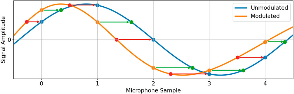
FIGURE 5. Methods of obtaining the unmodulated signal (blue) from the modulated signal (orange): The orange sampling points can be time-shifted to their equivalent positions on the blue graph (green points) and subsequently the blue points are obtained by interpolation. Alternatively, the equivalent positions of the blue points on the orange graph (red points) can be interpolated first and subsequently time-shifted to obtain the blue points.

To obtain the timestamps of the red points, we must compute the time of arrival of wavefronts sampled by M_S at M_M. As before, we simplify the microphone movement to a non-uniform linear movement by projecting it onto the red line from Figure 2. We now define this red line as an axis with its origin at the origin of the coordinate system and its positive direction pointing away from the source of the plane waves. Let us further assume that a given wavefront arrives at M_S at time t₀ and reaches M_M after an additional t₀-and DOA-dependent time Δt_SM(t₀, φ, θ) (which may also be negative). The location of M_M on the red axis can now be expressed as −r ⋅ sin(θ) ⋅ cos (2πf_rot (t₀ + Δt_SM(t₀, φ, θ)) − φ). Additionally, the Δt_SM(t₀, φ, θ)-dependent position of the wavefront on the red axis is given by c ⋅Δt_SM(t₀, φ, θ), since it reaches the origin at time t₀. We can now obtain Δt_SM(t₀, φ, θ) by equating the location of M_M and the wavefront on the red axis as −r ⋅ sin(θ) ⋅ cos (2πf_rot (t₀ + Δt_SM(t₀, φ, θ)) − φ) = c ⋅Δt_SM(t₀, φ, θ). Unfortunately, Δt_SM(t₀, φ, θ) cannot be solved analytically, therefore we instead obtain this value by optimization:

$\mathrm{\Delta }{t}_{\text{SM}}\left(t_0,\phi ,\theta \right)=\underset{\mathrm{\Delta }{t}_{\text{SM}}\left(t_0,\phi ,\theta \right)}{\mathrm{argmin}}(|r\cdot \sin \left(\theta \right)\cdot \cos \left(2\pi f_{\mathit{rot}}\left(t_0+\mathrm{\Delta }{t}_{\text{SM}}\left(t_0,\phi ,\theta \right)\right)-\phi \right)+c\cdot \mathrm{\Delta }{t}_{\text{SM}}\left(t_0,\phi ,\theta \right)|).(8)$

Note that it can be shown that the computation of Δt_SM(t₀, φ, θ) is unique as long as the microphone movement does not exceed the speed of sound.

Unmodulating an arbitrary signal x(t) for a given DOA (φ, θ) can now be performed using the following algorithm:

Algorithm 1.Frequency Unmodulation Algorithm

1: Compute Δt_SM(t₀, φ, θ) by optimizing Eq. 8 for all sample timestamps t₀

2: Calculate the frequency unmodulated timestamps ${\widehat{t}}_{\text{FU}}(t_0,\phi ,\theta )\leftarrow t_0+\mathrm{\Delta }{t}_{\text{SM}}(t_0,\phi ,\theta )$

3: Interpolate x(t) at positions $x({\widehat{t}}_{\text{FU}}(t_0,\phi ,\theta ))$ using Eq. 7

4: Return the frequency unmodulated signal $y(t_0,\phi ,\theta )\leftarrow x({\widehat{t}}_{\text{FU}}(t_0,\phi ,\theta ))$

Despite the ability of the above algorithm to accurately unmodulate a given signal, its direct implementation is slow due to the requirement of solving an optimization problem for each sample and the utilized interpolation method. To speed up the algorithm, we define a frequency unmodulation matrix Z_FU(φ, θ) which unmodulates a signal x = [x₀ x₁ … x_L−1] of length L, where x_i corresponds to the ith microphone sample, for a given DOA via vector-matrix multiplication. This operation can be performed both in the time domain and in the frequency domain. We perform this operation in the frequency domain as

${\mathbf{y}}_{\text{FU}}\left(\phi ,\theta \right)={\text{RFFT}}^{-1}\left\{\text{RFFT}\left\{\mathbf{x}\right\}\cdot {\mathbf{Z}}_{\text{FU}}\left(\phi ,\theta \right)\right\},(9)$

where y_FU(φ, θ) is the frequency unmodulated signal for the given DOA and RFFT{⋅} represents the L-length real-valued Fast Fourier Transform, i.e., the input data is assumed to be real and due to symmetric properties of the complex spectrum only the first n = L/2 + 1 complex frequency bins are computed and returned as a row vector. It is now evident why we choose to perform unmodulation in the frequency domain, since the required dimensions of Z_FU(φ, θ) in the frequency domain are n × n as opposed to L × L in the time domain. This results in an approximately four-fold decrease in the number of computations required for the vector-matrix multiplication.

It is important to note that the usage of the Fast Fourier Transform algorithm requires the length of the input signal L to be a power of two. Furthermore, we assume that RFFT{⋅} applies a scaling factor of 2/L and no scaling is applied by RFFT⁻¹{⋅}.

To obtain Z_FU(φ, θ) we define a function $f(k,t)=A_k\cdot \cos (2\pi k\frac{f_s}{L}t+{\phi }_{\text{k}})$ and subsequently construct a set of vectors as ${\mathbf{x}}_k=[f(k,0)f(k,\frac{1}{f_s})\dots f(k,\frac{L-1}{f_s})]$ for k ∈ [0, 1, … , n − 1]. Each vector x_k contains the first L samples of the center frequencies of the kth RFFT frequency bin (with amplitude A_k and phase offset φ_k) which have been sampled at sampling rate f_s. When computing the magnitude spectra of x_k as |RFFT{x_k}| using a rectangular window, we obtain spectra which appear to have no spectral leakage, i.e., $|\text{RFFT}{\{{\mathbf{x}}_k\}}_k|=A_k$, where RFFT{⋅}_k denotes the kth element of the vector returned by RFFT, and $|\text{RFFT}{\{{\mathbf{x}}_k\}}_{i\ne k}|=0$ for i ∈ [0, 1, … , n − 1]. Similarly, the phase spectra ∠RFFT{x_k} correspond to $\angle \text{RFFT}{\{{\mathbf{x}}_k\}}_k={\phi }_k$ and are indeterminate at the remaining bins. Note that in reality the spectra do have spectral leakage, however, the nulls of the sidelobes fall exactly onto the frequency bins evaluated by RFFT{⋅}. The previously mentioned properties do not hold for other window functions, since they produce a main lobe that spreads to the evaluated neighboring frequency bins. Therefore, we assume that RFFT{⋅} and RFFT⁻¹{⋅} utilize a rectangular window function.

We now define another function $g(k,t)=f(k,t){|}_{A_k=1,{\phi }_k=0}=\cos (2\pi k\frac{f_s}{L}t)$ and construct a set of vectors by sampling g (k, t) at times $t={\widehat{t}}_{\text{FU}}(\frac{i}{f_s},\phi ,\theta )$ for i ∈ [0, 1, … , L − 1] and k ∈ [0, 1, … , n − 1]. The times ${\widehat{t}}_{\text{FU}}(\cdot )$ are given by step (1) of the above algorithm and are computed for the given DOA (φ, θ). The resulting vectors can be expressed as

${\mathbf{z}}_{{\text{FU}}_k}\left(\phi ,\theta \right)=\left[g\left(k,{\widehat{t}}_{\text{FU}}\left(0,\phi ,\theta \right)\right)g\left(k,{\widehat{t}}_{\text{FU}}\left(\frac{1}{f_s},\phi ,\theta \right)\right)\dots g\left(k,{\widehat{t}}_{\text{FU}}\left(\frac{L-1}{f_s},\phi ,\theta \right)\right)\right]$

and represent the signals that are obtained when the unmodulation algorithm is applied to the center frequencies of each frequency bin with unit amplitude and no phase offset. An example plot of $|\text{RFFT}\{{\mathbf{z}}_{{\text{FU}}_{341}}(0,\frac{\pi }{2})\}|$ and |RFFT{x₃₄₁}| for L = 8,192, A₃₄₁ = 0.5, φ₃₄₁ = 0 and f_rot = 42 Hz is depicted in Figure 6. Given that the magnitude spectrum of x_k is concentrated onto the kth frequency bin and the magnitude spectrum of ${\mathbf{z}}_{{\text{FU}}_k}(\phi ,\theta )$ represents the unmodulated counterpart of the kth frequency bin with unit amplitude, we can unmodulate the magnitude spectrum of x_k for the DOA (φ, θ) by computing $|\text{RFFT}{\{{\mathbf{x}}_k\}}_k|\cdot |\text{RFFT}\{{\mathbf{z}}_{{\text{FU}}_k}(\phi ,\theta )\}|$. Similarly, the phase spectrum of x_k can be unmodulated by $\angle \text{RFFT}{\{{\mathbf{x}}_k\}}_k+\angle \text{RFFT}\{{\mathbf{z}}_{{\text{FU}}_k}(\phi ,\theta )\}$. Combining these properties allows for unmodulation of the spectrum of x_k by computing $\text{RFFT}{\{{\mathbf{x}}_k\}}_k\cdot \text{RFFT}\{{\mathbf{z}}_{{\text{FU}}_k}(\phi ,\theta )\}$, which is equivalent to scaling the spectrum of ${\mathbf{z}}_{{\text{FU}}_k}(\phi ,\theta )$ by the phasor $A_k\cdot e^{i{\phi }_k}$.

FIGURE 6

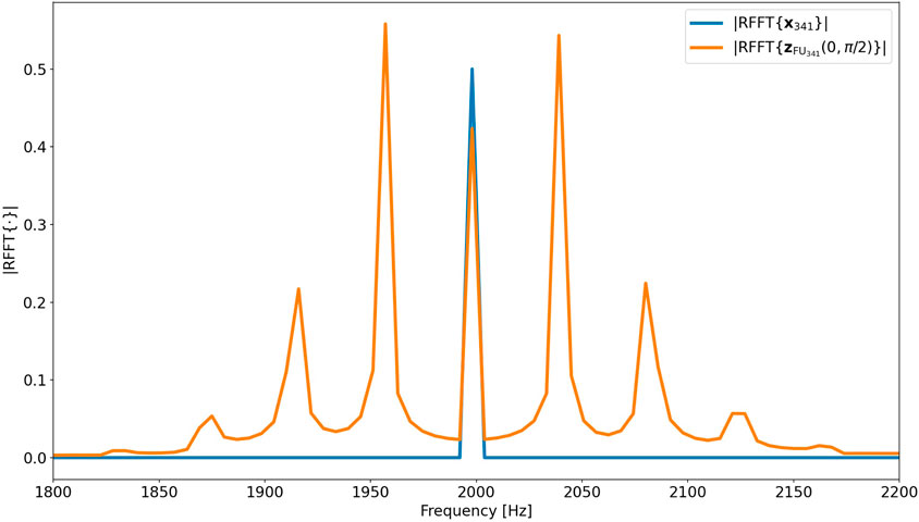
FIGURE 6. Example plot of |RFFT{x₃₄₁}| and $|\text{RFFT}\{{\mathbf{z}}_{{\text{FU}}_{341}}(0,\frac{\pi }{2})\}|$ for L = 8,192, f_s = 48 kHz, A₃₄₁ = 0.5, φ₃₄₁ = 0, f_rot = 42 Hz and r = 0.045 m.

These considerations can now be extended to more general source signals x. Since the spectrum of x is fully characterized by the amplitudes A_k and the phases φ_k of every RFFT bin, we can unmodulate each frequency bin individually using the corresponding spectra of ${\mathbf{z}}_{{\text{FU}}_k}(\phi ,\theta )$. The unmodulated signal y_FU(φ, θ) can then be obtained by computing the sum of the unmodulated spectra of each frequency bin and subsequently applying RFFT⁻¹ as:

${\mathbf{y}}_{\text{FU}}\left(\phi ,\theta \right)={\text{RFFT}}^{-1}\left\{{\displaystyle \sum _{k=0}^{n-1}}\text{RFFT}{\left\{\mathbf{x}\right\}}_k\cdot \text{RFFT}\left\{{\mathbf{z}}_{{\text{FU}}_k}\left(\phi ,\theta \right)\right\}\right\}.$

To represent this equation as the vector-matrix computation from Eq. 9 we can stack all ${\mathbf{z}}_{{\text{FU}}_k}(\phi ,\theta )$ to form the unmodulation matrix Z_FU(φ, θ) as

${\mathbf{Z}}_{\text{FU}}(\phi ,\theta )=\left[\begin{array}{c}\hfill \text{RFFT}\{{\mathbf{z}}_{{\text{FU}}_1}(\phi ,\theta )\}\hfill \\ \hfill \text{RFFT}\{{\mathbf{z}}_{{\text{FU}}_2}(\phi ,\theta )\}\hfill \\ \hfill ⋮\hfill \\ \hfill \text{RFFT}\{{\mathbf{z}}_{{\text{FU}}_{n-1}}(\phi ,\theta )\}\hfill \end{array}\right].(10)$

The computational cost of deriving the matrices grows quadratically with L. The same holds for the number of computations necessary to apply the unmodulation matrix to the source signal. Therefore, it is desirable to keep L as low as possible, which incentivizes the usage of frame-wise processing of the source signal. The length of each frame cannot be decreased indefinitely, since inaccuracies occur close to the boundaries of each unmodulated frame. For this reason, subsequent frames must overlap to a certain extent. Additionally, if the shift between the frames is not carefully chosen, the initial microphone position at each frame will differ, resulting in a change in DOA between the initial microphone position and the sound source. This would require the computation of a different modulation or unmodulation matrix for each frame. This is circumvented by using a frame shift of S = f_s/f_rot samples. In case S is not an integer, the frame shift of each frame is chosen such that the start of the nth frame is at ⌊n ⋅ f_s/f_rot⌉ samples. To ensure a frame overlap of at least 25%, S < 0.75 ⋅ L must hold. Therefore, we set L = 2^k, where k represents the smallest integer for which S < 0.75 ⋅ 2^k holds. As an example, for f_s = 48 kHz and f_rot = 42 Hz the frame shift is S ≈ 1,143 samples and therefore the minimum required frame length is L = 2048. Unmodulating a signal for a given DOA now only requires the computation of a matrix of size 1,025 × 1,025 which is subsequently used to process each frame. The resulting time domain frames are added together using equal power crossfades at the overlapping sections.

When comparing the performance of matrix-based unmodulation with Algorithm 1, we find that matrix-based unmodulation is significantly faster, especially as the length of the audio signal increases. For instance, our Python implementation of matrix-based unmodulation requires approximately 0.12  s, 0.16  s and 0.53 s to process 1 s, 10  s and 100 s audio files at a rotational speed of f_rot = 42 Hz. This is in stark contrast with Algorithm 1, which requires around 8  s, 80  s and 800 s for the same audio files.

To unmodulate a signal for multiple colatitude angles requires the computation of an unmodulation matrix for each colatitude. Unmodulating for various azimuth angles, however, can be performed using only one unmodulation matrix computed at, for example, φ = 0. Unmodulation for other arbitrary azimuth angles φ can then be performed by omitting the first $\lfloor \frac{f_s}{f_{\text{rot}}}\cdot \frac{\phi }{2\pi }\rceil$ samples of the signal and subsequently using Z_FU(0, θ) to unmodulate each frame. Using these optimizations and assuming a perfectly constant rotational speed of f_rot = 42 Hz, our Python implementation is capable of unmodulating for 180 different azimuth angles in real-time.

3.2 Amplitude modulation compensation

To compensate for the amplitude modulation present in a signal for a given DOA we proceed in a similar manner to the matrix-based frequency unmodulation from the previous section. Given knowledge of the absolute value of the directivity D (f_m, φ_m, θ_m) and the frequency response H (f_m) we can generate a set of basis functions whose spectra represent the amplitude unmodulated counterparts of each frequency bin. We use the same function $g(k,t)=\cos (2\pi k\frac{f_s}{L}t)$ from the previous section and weight it by the reciprocal value of A₀ (t, f_src, φ, θ) from Eq. 6. The respective scaling factors A₀ are set to $A_0=1/|H(f_{\text{src}},0,\frac{\pi }{2})|$. We then construct a set of vectors ${\mathbf{z}}_{{\text{AU}}_k}(\phi ,\theta )$ by taking L samples of the weighted function at sampling rate f_s for k ∈ [0, 1, … , n − 1]. The resulting set of vectors can be expressed as

${\mathbf{z}}_{{\text{AU}}_k}\left(\phi ,\theta \right)=\left[\frac{1}{A_{0_k}\left(0\right)}\cdot g\left(k,0\right)\frac{1}{A_{0_k}\left(\frac{1}{f_s}\right)}\cdot g\left(k,\frac{1}{f_s}\right)\dots \frac{1}{A_{0_k}\left(\frac{L-1}{f_s}\right)}\cdot g\left(k,\frac{L-1}{f_s}\right)\right],$

where $A_{0_k}(t)=A_0(t,k\frac{f_s}{L},\phi ,\theta )$. To form the amplitude unmodulation matrix we stack all ${\mathbf{z}}_{{\text{AU}}_k}(\phi ,\theta )$ in a similar manner to Eq. 10 to form the amplitude unmodulation matrix Z_AU (φ, θ). The amplitude unmodulated signal y_AU (φ, θ) for DOA (φ, θ) can then be obtained by

${\mathbf{y}}_{\text{AU}}\left(\phi ,\theta \right)={\text{RFFT}}^{-1}\left\{\text{RFFT}\left\{\mathbf{x}\right\}\cdot {\mathbf{Z}}_{\text{AU}}\left(\phi ,\theta \right)\right\}.$

We can now combine Z_AU (φ, θ) and Z_FU(φ, θ) into an unmodulation matrix Z_U (φ, θ), given by

${\mathbf{Z}}_{\text{U}}\left(\phi ,\theta \right)={\mathbf{Z}}_{\text{AU}}\left(\phi ,\theta \right)\cdot {\mathbf{Z}}_{\text{FU}}\left(\phi ,\theta \right),(11)$

which enables simultaneous frequency and amplitude unmodulation. Note that frequency unmodulation is sensitive to amplitude variations due to the utilized interpolation. This is why Z_AU (φ, θ) is positioned to the left of Z_FU(φ, θ) in Eq. 11.

3.3 Modulation algorithm

An algorithm that modulates an arbitrary signal for a given DOA, i.e., the inverse of the unmodulation algorithm, is beneficial for simulation purposes. Let us revisit the moving microphone M_M and the stationary microphone M_S from Section 3.1. A signal can be frequency modulated for a given DOA by interpolating the green points in Figure 5 from the blue points and equally spacing the interpolated points to obtain the orange points. The timestamps of the green points are computed by calculating the time of arrival of wavefronts sampled by M_M at M_S. Let us assume a given wavefront arrives at M_M at time t₀. At this point in time, the position of M_M along the red axis from Figure 2 can be expressed as −r ⋅ sin(θ) ⋅ cos (2πf_rot t₀ − φ). As the wavefront travels along this axis at the speed of sound, the time Δt_MS(t₀, φ, θ) required for the wavefront to reach M_S corresponds to

$\mathrm{\Delta }{t}_{\text{MS}}\left(t_0,\phi ,\theta \right)=\frac{r\cdot \sin \left(\theta \right)\cdot \cos \left(2\pi f_{\mathit{rot}}{t}_0-\phi \right)}{c}.$

Therefore, to frequency modulate an arbitrary signal for a given DOA, we follow the same steps as in Algorithm 1, but we omit step 1 and replace ${\widehat{t}}_{\text{FU}}(t_0,\phi ,\theta )$ by ${\widehat{t}}_{\text{FM}}(t_0,\phi ,\theta )=t_0+\mathrm{\Delta }{t}_{\text{MS}}(t_0,\phi ,\theta )$.

A frequency modulation matrix Z_FM(φ, θ) can now be formulated in a similar fashion to Z_FU(φ, θ) from Eq. 9 by stacking the set of vectors ${\mathbf{z}}_{{\text{FM}}_k}(\phi ,\theta )$ given by

${\mathbf{z}}_{{\text{FM}}_k}\left(\phi ,\theta \right)=\left[g\left(k,{\widehat{t}}_{\text{FM}}\left(0,\phi ,\theta \right)\right)g\left(k,{\widehat{t}}_{\text{FM}}\left(\frac{1}{f_s},\phi ,\theta \right)\right)\dots g\left(k,{\widehat{t}}_{\text{FM}}\left(\frac{L-1}{f_s},\phi ,\theta \right)\right)\right].$

Here the times ${\widehat{t}}_{\text{FM}}(\cdot )$ are given by the previously described frequency modulation algorithm and the function g (⋅) is given in Section 3.1. Note that Z_FM(φ, θ) cannot be obtained by inverting Z_FU(φ, θ) or vice versa since both Z_FU(φ, θ) and Z_FM(φ, θ) feature very large condition numbers for inversion.

The amplitude modulation matrix Z_AM(φ, θ) can be formed in a similar manner to Z_AU (φ, θ) by stacking the set of vectors ${\mathbf{z}}_{{\text{AM}}_k}(\phi ,\theta )$ given by

${\mathbf{z}}_{{\text{AM}}_k}\left(\phi ,\theta \right)=\left[A_{0_k}\left(\frac{1}{f_s}\right)\cdot g\left(k,0\right)A_{0_k}\left(\frac{1}{f_s}\right)\cdot g\left(k,\frac{1}{f_s}\right)\dots A_{0_k}\left(\frac{L-1}{f_s}\right)\cdot g\left(k,\frac{L-1}{f_s}\right)\right].$

where $A_{0_k}(t)=A_0(t,k\frac{f_s}{L},\phi ,\theta )$.

Simultaneous amplitude and frequency modulation can be performed using the modulation matrix Z_M(φ, θ) given by Z_M(φ, θ) = Z_FM(φ, θ) ⋅Z_AM(φ, θ). Note that frequency modulation is sensitive to amplitude variations due to the utilized interpolation. This is why Z_AM(φ, θ) is positioned to the right of Z_FM(φ, θ).

3.4 Direction of arrival estimation

To estimate the azimuth angle of incoming sound sources, we compute ${\mathbf{Z}}_{\text{U}}(0,\frac{\pi }{2})$ and unmodulate a given source signal for an arbitrary number of DOA angles φ ∈ [0, 2π) using the optimization discussed at the end of Section 3.1. We then estimate the PSD of each unmodulated signal $\mathbf{y}(\phi ,\frac{\pi }{2})$ in a frame-wise manner using both a long frame length of L = 8,192 and a short frame length of L = 128. The PSD is estimated by computing the squared magnitude of the RFFT of $\mathbf{y}(\phi ,\frac{\pi }{2})$ which has been windowed using a Blackman window. The frame shift is chosen such that there is one frame for each microphone rotation for L = 8,192 and 30 frames for each microphone rotation for L = 128. We will express the ith PSD frame of the unmodulated signals using a long frame length as ${\mathbf{S}}_{\mathbf{yy}}^{\text{l}}(i,\phi ,\frac{\pi }{2})$ and the one utilizing a short frame length as ${\mathbf{S}}_{\mathbf{yy}}^{\text{s}}(i,\phi ,\frac{\pi }{2})$. The azimuth angle can now be estimated for each microphone rotation p in two different ways: One method is to compute the focusedness F (i, φ) of ${\mathbf{S}}_{\mathbf{yy}}^{\text{l}}(i,\phi ,\frac{\pi }{2})$ for all i and φ using Eq. 5. Subsequently, the azimuth estimate is determined for each i by finding the value of φ for which F (i, φ) attains its maximum. By setting i = p we obtain the estimates for each microphone rotation since the frame shift was selected such that there is one frame for each microphone rotation. We will denote the focusedness-based estimate for the pth microphone rotation as ${\widehat{\phi }}_F(p)$.

The second azimuth estimation method is to compute the energy E^s (i, φ) of ${\mathbf{S}}_{\mathbf{yy}}^{\text{s}}(i,\phi ,\frac{\pi }{2})$ for all i and φ as $E^{\text{s}}(i,\phi )={\sum }_{k=0}^{N/2}{S}_{{\mathbf{yy}}_n}^{\text{s}}{(i,\phi ,\frac{\pi }{2})}_k$ and subsequently calculate the variance V (p, φ) of E^s (i, φ) over the pth microphone rotation as

$V\left(p,\phi \right)=\text{Var}\left(E^{\text{s}}\left(30p,\phi \right),E^{\text{s}}\left(30p+1,\phi \right),\dots ,E^{\text{s}}\left(30p+29,\phi \right)\right).$

The azimuth estimate for the pth microphone rotation corresponds to the value of φ for which V (p, φ) has its minimum value for a given p. We will denote the variance-based estimates as ${\widehat{\phi }}_V(p)$.

There are numerous possibilities of combining all ${\widehat{\phi }}_F(p)$ and ${\widehat{\phi }}_V(p)$ into one final DOA prediction. For the sake of simplicity we choose to compute two weighted histograms, one for all ${\widehat{\phi }}_F(p)$ and the other for ${\widehat{\phi }}_V(p)$, where the weights are given by $F(p,{\widehat{\phi }}_F(p))$ and $V(p,{\widehat{\phi }}_V(p))$, respectively. The histograms are computed using weighted Parzen window density estimation with a kernel size of $\frac{1}{6}\pi$ radians. This kernel size was chosen empirically as we found it provided a good trade-off between the detail and the smoothness of the histograms. Both histograms are subsequently multiplied with each other to obtain a combined histogram. The maximum value of the combined histogram represents the final azimuth angle estimate.

As an example, assume a 2 kHz sine wave arrives at the rotating microphone at DOA $(\pi ,\frac{\pi }{2})$ and the microphone rotation is set to f_rot = 42 Hz. The recorded signal can be simulated by transforming a sampled 2 kHz sine wave with ${\mathbf{Z}}_{\text{M}}(\pi ,\frac{\pi }{2})$. We now unmodulate this signal for 360 uniformly spaced values of φ. Since the microphone takes approximately 1,143 samples within each rotation, the ith unmodulated signal is obtained by omitting the first $\lfloor \frac{1143}{360}\rceil \cdot i$ samples of the recorded signal and subsequently transforming the truncated signal with ${\mathbf{Z}}_{\text{U}}(\pi ,\frac{\pi }{2})$ in a frame-wise manner. The PSDs ${\mathbf{S}}_{\mathbf{yy}}^{\text{l}}(0,\phi ,\frac{\pi }{2})$ of the unmodulated signals are depicted in Figure 7A. It can be observed that as the azimuth angle approaches the correct value, all sidebands of the 2 kHz sine wave gradually disappear. Furthermore, the focusedness F (0, φ) of ${\mathbf{S}}_{\mathbf{yy}}^{\text{l}}(0,\phi ,\frac{\pi }{2})$ exhibits a clear peak at φ = π, as depicted in Figure 7C. A plot of the energy E^l (0, φ) of ${\mathbf{S}}_{\mathbf{yy}}^{\text{l}}(0,\phi ,\frac{\pi }{2})$ is included in the same figure, which, unlike our findings from Section 2.2, does not remain constant. This is caused by amplitude unmodulation, as it does not represent an energy-conserving transformation. To correct this inconsistency, we multiply each F (i, φ) by ${\bar{E}}^{\text{l}}{(i)}^2/E^{\text{l}}{(i,\phi )}^2$, where ${\bar{E}}^{\text{l}}(i)$ represents the mean of E^l (i, φ). The corrected plots of F (0, φ) and E^l (0, φ) are shown in Figure 7C. Moreover, a plot of the energy E^s (i, φ) of ${\mathbf{S}}_{\mathbf{yy}}^{\text{s}}(i,\phi ,\frac{\pi }{2})$ is depicted in Figure 7B for one microphone rotation. As it can be observed, the energies become more uniform over time as φ approaches the correct angle. The variance V (0, φ) of E^s (i, φ) also exhibits a clear minimum at φ = π, as depicted in Figure 7C.

FIGURE 7

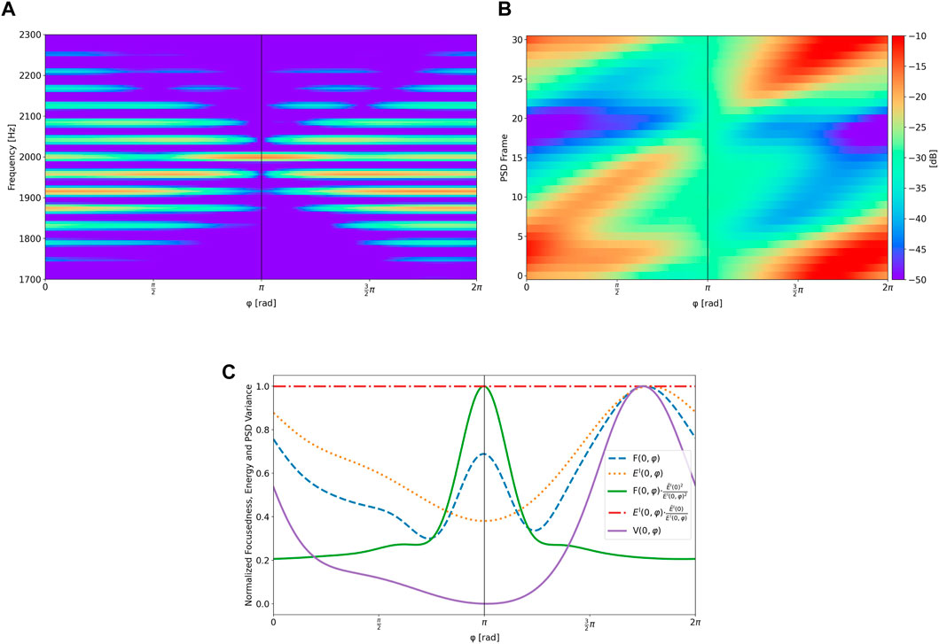
FIGURE 7. Analysis of unmodulated versions of a modulated 2 kHz sine wave with DOA $(\pi ,\frac{\pi }{2})$ using long and short frame lengths. All plots in (C) have been normalized by dividing each graph by its maximum value. The solid lines have a maximum and a minimum at φ = π and are used for DOA estimation. (A) Plot of $S_{yy}^1\left(0,\phi ,\frac{\pi }{2}\right)$. (B) Plot of $E^S(i,\phi )$. (C) Energy, focusedness and PSD variance.

To enable localization of multiple and wideband acoustic sources, both ${\mathbf{S}}_{\mathbf{yy}}^{\text{l}}(i,\phi ,\frac{\pi }{2})$ and ${\mathbf{S}}_{\mathbf{yy}}^{\text{s}}(i,\phi ,\frac{\pi }{2})$ are decomposed into 32 subbands using a logarithmic filterbank. We then compute the focusedness F (n, p, φ), the correction factors $\bar{E}{(n,p)}^2/E{(n,p,\phi )}^2$ and the variances V (n, p, φ) for each subband n, microphone rotation p, and azimuth angle φ. The estimates ${\widehat{\phi }}_F(n,p)$ and ${\widehat{\phi }}_V(n,p)$ for each subband and microphone rotation are now given by:

${\widehat{\phi }}_F\left(n,p\right)=\underset{\phi }{\text{argmax}}\left(F\left(n,p,\phi \right)\cdot \frac{\bar{E}{\left(n,p\right)}^2}{E{\left(n,p,\phi \right)}^2}\right),{\widehat{\phi }}_V\left(n,p\right)=\underset{\phi }{\mathrm{arg\; min}}\left(V\left(n,p,\phi \right)\right).$

The final DOA predictions are made by multiplying the weighted histograms of ${\widehat{\phi }}_F(n,p)$ and ${\widehat{\phi }}_V(n,p)$ with each other and finding peaks in the resulting combined histogram. The histogram computation follows the previously described weighted Parzen window density estimation and the histogram weights are given by $F(n,p,{\widehat{\phi }}_F(n,p))\cdot \bar{E}{(n,p)}^2/E{(n,p,{\widehat{\phi }}_F(n,p))}^2$ and $V(n,p,{\widehat{\phi }}_V(n,p))$, respectively. The resulting combined histogram is then analyzed to find one or multiple peaks. If the number of sources k is known, the predictions correspond to the k tallest peaks of the histogram. However, if the number of sources is unknown, more advanced algorithms are required to determine the number of audio sources, such as those presented in Yamamoto et al. (2003).

After one or multiple azimuth predictions $\widehat{\phi }$ have been made, the colatitude can be estimated similarly by computing ${\mathbf{S}}_{\mathbf{yy}}^{\text{l}}(i,\widehat{\phi },\theta )$ and ${\mathbf{S}}_{\mathbf{yy}}^{\text{s}}(i,\widehat{\phi },\theta )$ for each $\widehat{\phi }$ and an arbitrary number of colatitude angles θ ∈ [0, π]. The colatitude estimates $\widehat{\theta }$ can then be obtained by computing

${\widehat{\theta }}_F\left(n,p\right)=\underset{\theta }{\text{argmax}}\left(F\left(n,p,\theta \right)\cdot \frac{\bar{E}{\left(n,p\right)}^2}{E{\left(n,p,\theta \right)}^2}\right),{\widehat{\theta }}_V\left(n,p\right)=\underset{\theta }{\mathrm{arg\; min}}\left(V\left(n,p,\theta \right)\right)$

and subsequently finding peaks in the combined weighted histograms of ${\widehat{\theta }}_F(n,p)$ and ${\widehat{\theta }}_V(n,p)$. Note that signals arriving at $\theta =\frac{\pi }{2}\pm {\theta }^{\prime }$ for ${\theta }^{\prime }\in [0,\frac{\pi }{2}]$ can only be distinguished from each other if the microphone directivity differs for these angles since the induced frequency modulation is identical for $\theta =\frac{\pi }{2}\pm {\theta }^{\prime }$.

4 Evaluation

To verify the accuracy of the presented algorithm both simulations and practical experiments have been conducted for one and two acoustic sources placed at various locations. The signals used for localization include simple pure tone test signals ranging from 125 Hz to 8 kHz; more complex test signals, i.e., a combination of all those pure tones, an exponential sine sweep, and pink noise; and real-world signals, i.e., male speech, female speech, a drum groove and an excerpt from a piano concerto. All samples are amplitude-normalized and have a length of approximately 2 s.

4.1 Simulation

We perform simulations for rotational speeds of 24 Hz and 42 Hz, since these values correspond to the minimum and maximum speeds of our REM prototype. To simulate the modulated signals we compute the modulation matrix ${\mathbf{Z}}_{\text{M}}(\phi ,\frac{\pi }{2})$ for each rotational speed and loudspeaker location(s) of interest and subsequently use these matrices to modulate the signals from the left column of Table 1. We use the direction-dependent magnitude response $|H(f_m,{\phi }_m,\frac{\pi }{2})|$ of our REM prototype to model the amplitude modulation of the amplitude modulation matrix. These magnitude responses were measured at 72 equidistant values of φ_m and all remaining values are interpolated using linear interpolation. Additionally, we apply smoothing to the interpolated $|H(f_m,{\phi }_m,\frac{\pi }{2})|$, since we found this substantially reduces artifacts introduced by the modulation and unmodulation algorithm. The radius for the computation of the matrices is selected as r = 0.045 m, since this value corresponds to the rotational radius of our REM prototype. Note that following the constraints at the end of Section 3.1 the size of the modulation and unmodulation matrices is 2049 × 2049 for f_rot = 24 Hz and 1,025 × 1,025 for f_rot = 42 Hz. As a consequence, the higher rotational speed leads to an approximately four-fold increase in the algorithm’s speed.

TABLE 1

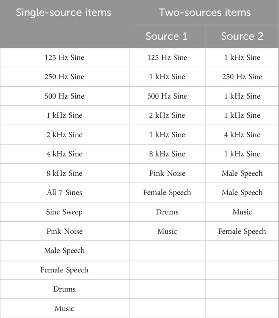
TABLE 1. Used audio samples for single source and two source localization.

To determine the robustness of the algorithm in the presence of noise, randomly generated pink noise is added to each modulated signal at various levels of signal-to-noise ratio (SNR). We employ pink noise as it closely resembles the wind noise that occurs during the microphone rotation. The noise level is adjusted relative to the modulated pink noise signal and mixed with the other signals at the same amplitude.

4.1.1 Single source localization

All signals from the left column of Table 1 are modulated for a DOA of $\phi =\frac{\pi }{2}$ and φ = π and subsequently mixed with pink noise at SNRs ranging from −20 dB to 20 dB. The noise in each signal is then reduced using spectral subtraction, given an estimate of the average noise spectrum obtained from a 1 s noise sample. Each filtered signal is subsequently unmodulated for 360 equidistant azimuth angles using the respective unmodulation matrices. Finally, the estimates ${\widehat{\phi }}_F(n,p)$ and ${\widehat{\phi }}_V(n,p)$ are computed for each unmodulated signal and combined into one histogram, whose largest peak corresponds to the final DOA estimate $\widehat{\phi }$.

To quantify the accuracy of the proposed DOA estimation method we compute the absolute DOA estimation error for each modulated signal. We average the results for $\phi =\frac{\pi }{2}$ and φ = π, as no notable difference in accuracy was observed for different source positions. The results can be found in Figure 8 for errors up to 60°. It can be observed that beyond 10 dB SNR all signals are localized with high accuracy, with the drums signal producing the worst results with a mean absolute error of 22 and 14° for f_rot = 24 Hz and f_rot = 42 Hz, respectively. In the case of single-frequency sources the microphone’s rotational speed has little impact on localization accuracy. For lower frequencies the error approximately halves for each doubling in frequency and frequencies above 500 Hz are localized accurately down to −20 dB. The increase in localization accuracy at higher frequencies can be attributed to a corresponding increase in distortion, which results in a greater discernibility between unmodulated signals associated with good and bad DOA candidates. In the case of wideband sources the localization accuracy at f_rot = 42 Hz is approximately half that of f_rot = 24 Hz above an SNR of 10 dB. Higher rotational speeds introduce more distortion, making it easier to differentiate between good and bad DOA candidates. However, these additional distortions appear to provide no benefit for single frequency source localization. Additionally, our results indicate that wideband signals with a more tonal and stationary nature exhibit greater localization accuracy, whereas signals with a percussive nature demonstrate lower localization accuracy. This is due to the focusedness measure implicitly requiring the input signal to be constant during each spectrogram frame. This also explains why the exponential sine sweep sees no improvement in error beyond −10 dB, since the signal is not constant during any spectrogram frame.

FIGURE 8

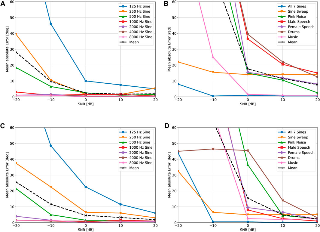
FIGURE 8. Simulated localization accuracy for various source signals, rotational speeds and SNRs. (A) Monochromatic results for f_rot = 24 Hz. (B) Wideband results for f_rot = 24 Hz. (C) Monochromatic results for f_rot = 42 Hz. (D) Wideband results for f_rot = 42 Hz.

4.1.2 Localization of two sources

To simulate two sources arriving from different directions, we modulate the signals from the center column of Table 1 for $\phi =\frac{\pi }{2}$ and the signals from the right column for $\phi =\frac{5}{8}\pi$, φ = π and $\phi =\frac{3}{2}\pi$. The modulated signals are subsequently added together, resulting in an angular separation between the simulated loudspeakers of 22.5, 90 and 180°, respectively. The combined signals are then mixed with pink noise at an SNR of 0 dB. Localization is again performed by reducing the noise using spectral subtraction, unmodulating the signal and computing the combined histogram of the focusedness- and spectrogram variance-based DOA estimates. The final DOA estimates correspond to the tallest and second-tallest peaks in the resulting histograms. The results are displayed in Table 2. Note that we assigned the detected peaks to the true peaks such that the combined error of both peaks is minimized. Furthermore, we assume that we have no knowledge which histogram peak is produced by which signal.

TABLE 2

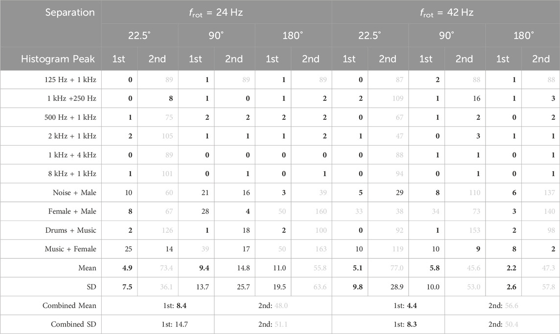
TABLE 2. Simulated absolute localization error for two acoustic sources at 0 dB SNR, given in degrees. The combined mean and standard deviation (SD) refer to the mean absolute error of all first and second peaks, respectively. Values below 10 are highlighted in bold, while values above 30 are shaded in grey.

For f_rot = 24 Hz the tallest histogram peak exhibits an average combined error of 8.4° for all speaker separations. The minimum error of 4.9° is observed at the smallest speaker separation, which is likely due to the merging of histogram peaks. This is supported by the fact that the second histogram peak is incorrect in most cases at 22.5° speaker separation, resulting in an average error of 73.4°. The maximum error of 11.0° of the first peak is observed at the largest speaker separation. However, it is important to note that this error is heavily impacted by two outliers, namely, the “Female + Male” and “Music + Female” signal combinations. The second histogram peak is precise for single-frequency sources above 125 Hz and for speaker separations above 22.5°. These sources can be localized well since their spectra do not overlap. In the case of wideband sources, localization of both sources is only accurate at 90° speaker separation with errors of 9.4 and 14.8° for the first and second histogram peaks, respectively. Localization of the second source at 180° speaker separation likely fails since, in each subband, one signal creates a maximum focusedness and spectrogram variance value where the other source creates a minimum. This increases the likelihood of one signal overpowering the other, leading to the failure of localization of the weaker signal. We hypothesize that for certain signal combinations this effect results in the detection of neither signal, as it was observed for the “Female + Male” and “Music + Female” signal combinations.

Similar results are obtained at a rotational speed of f_rot = 42 Hz, however, there are two notable differences: The average combined error of the tallest histogram peak is significantly lower at 4.4°. This is likely caused by the previously discovered improvements in single source localization accuracy at higher rotational speeds. The second difference is that localization of the second source is less precise for wideband sources on average. We hypothesize that this is caused by a larger spectral spread of the signals at the higher rotational speed, resulting in more interference between the signals in each subband. We therefore conclude that localization of two sources benefits from a lower rotational speed.

4.2 Measurements

All practical measurements were captured with our REM prototype, as depicted in Figure 9, which was placed at a height of 1.2 m in a low-reverberant room with dimensions W× L× H = 2.75 m × 2.5 m × 2.4 m. In contrast to the simulation we not only captured data at rotational speeds of 24 Hz and 42 Hz, but additionally employed a rotational speed of 34 Hz. The choice of 34 Hz was made to balance the trade-off between the increase in single source localization accuracy for higher rotational speeds and the increase in self-induced noise. All signals were played at the same volume by loudspeakers situated approximately 1.3 m from the REM within the rotational plane. The SNR between the pink noise signal and the microphone’s self-induced noise was measured as approximately 1 dB, −2.5 dB and −6.5 dB for the three rotational speeds. More details regarding the recording setup can be found in Lawrence (2023).

FIGURE 9

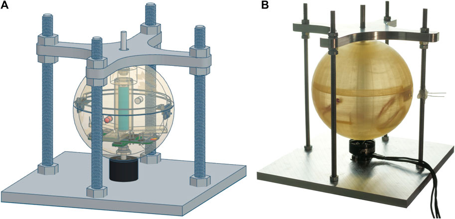
FIGURE 9. 3D-model (A) and photograph (B) of the REM prototype.

Note that, as opposed to the simulation, the microphone’s rotational speed is not perfectly constant in practice. As a consequence, it is necessary to compute multiple unmodulation matrices to account for these fluctuations, which leads to a significant reduction in the algorithm’s speed. Future hardware improvements are expected to help overcome this issue.

4.2.1 Single source localization

The loudspeakers were placed in the same positions as for the simulation. The noise in the captured signals is reduced using spectral subtraction, given a 1 s noise sample captured immediately before the signal was played. Each filtered signal is subsequently unmodulated for 360 equidistant azimuth angles and the DOA estimates are computed. The results are again averaged for $\phi =\frac{\pi }{2}$ and φ = π, since no notable difference in localization accuracy could be observed for different loudspeaker placements, and are displayed in Figure 10. Localization of single-frequency signals is successful at all rotational speeds except for the 125 Hz and the 500 Hz signals. While the inability to localize the 125 Hz signal is consistent with our simulation, the 500 Hz signal presents an anomaly. We hypothesize that the non-anechoic conditions of our recording setup resulted in a standing wave at 500 Hz, which led to additional amplitude modulation as the microphone changed its position relative to the loudspeaker. Furthermore, it can be observed that, unlike our simulation, localization of higher frequencies is not always more accurate. We believe this error is caused by violations of the idealizing assumptions from Section 2, as well as inaccuracies within the microphone’s directivity measurements, which affect higher frequencies more heavily than low frequencies. The best average performance in single frequency localization is achieved at a rotational speed of f_rot = 34 Hz with a mean absolute error of 23°, which is significantly higher than the error range of 3–6° produced by the simulation at 0 dB. The other two rotational speeds exhibit a further increase in the mean absolute error by approximately 13°. Wideband sources are localized more accurately and reliably than single-frequency sources, indicating that the errors occurring in single frequency localization cancel each other out. The best average performance for wideband source localization is achieved at a rotational speed of f_rot = 34 Hz with a mean absolute error of 5.4°, which is significantly lower than the error range of 15–18° produced by the simulation at 0 dB. This is likely attributable to the fact that the harmonic noise present in the REM recordings is more effectively filtered by spectral subtraction than the additive pink noise from the simulation, resulting in a higher SNR after noise reduction. The mean absolute error at f_rot = 24 Hz and f_rot = 42 Hz is also better than the simulation at 10 and 6°, respectively. Given that the accuracy of both single-frequency and wideband localization is highest at a rotational frequency of f_rot = 34 Hz it can be inferred that there exists a trade-off between the increase in single source localization accuracy and the increase in self-induced noise for higher rotational speeds.

FIGURE 10

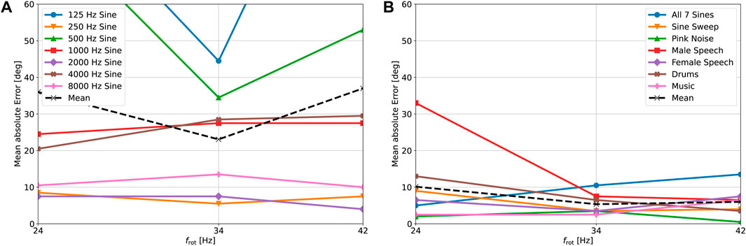
FIGURE 10. Real-world localization accuracy for various source signals and rotational speeds. (A) Results for single frequency signals. (B) Results for wideband signals.

4.2.2 Localization of two sources

Two loudspeakers were placed in the same locations as described in Section 4.1.2 and all signals were captured with the REM at the three previously mentioned rotational speeds. The noise in each captured signal is reduced using the same procedure as explained in the previous section and then the combined histogram is computed. The results for the tallest and second-tallest histogram peaks are shown in Table 3. The tallest histogram peak has an average combined error of 9.8° for f_rot = 24 Hz. This error increases to 12.3 and 13.0° for f_rot = 34 Hz and f_rot = 42 Hz, respectively. This suggests that for two sources the benefit of a higher rotational speed observed in Section 4.1.2 is offset by the drawback of a decrease in SNR at higher rotational speeds. The accuracy of the second histogram peak deteriorates with an increase in rotational speed in a similar manner to the first histogram peak. In the case of f_rot = 24 Hz the second peak exhibits an error of 38.5° which is lower than the error of 48.0° observed in the simulation. Especially in the case of 180° speaker separation there is a significant improvement for wideband signals. Again, this improvement can likely be attributed to more effective reduction of harmonic noise, rather than the reduction of pink noise. Additionally, the phenomenon observed in Section 4.1.2, where one signal dominates the other at the 180° speaker separation, seems to be less prominent in practical scenarios. The results for single frequency sources are not as accurate as the simulation for the same reasons as the inaccuracies observed in Figure 10A. Localization of the second source fails at 22.5° speaker separation for most signals and rotational speeds, with the exception of the “1 kHz + 4 kHz” and “8 kHz + 1 kHz” signals. It is hypothesized that these exceptions are caused by the inaccuracies from Figure 10A, preventing the merging of the histogram peaks. We conclude that both our simulations and practical experiments indicate that the lowest investigated rotational speed of f_rot = 24 Hz leads to the most accurate localization of two sources.

TABLE 3

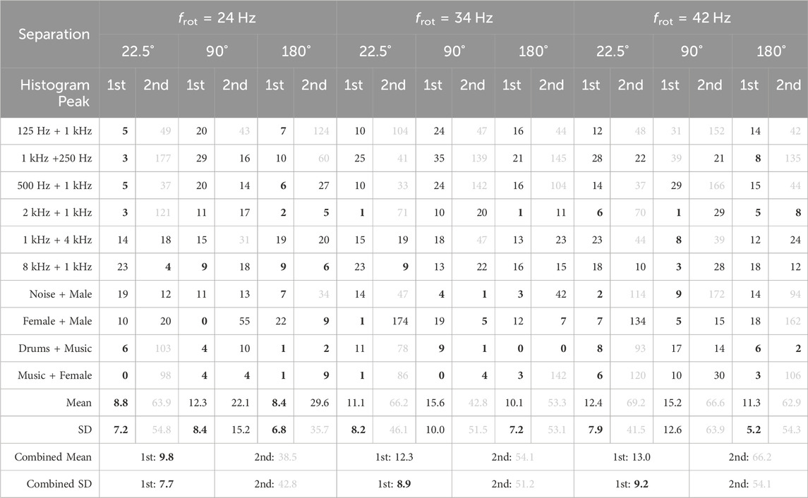
TABLE 3. Real-world absolute localization error for two acoustic sources, given in degrees. The combined mean and SD refer to the mean absolute error of all first and second peaks, respectively. Values below 10 are highlighted in bold, while values above 30 are shaded in grey.

5 Conclusion

We have presented a novel method for direction of arrival estimation of unknown sound sources using a single moving microphone. The method compensates for the induced frequency and amplitude modulation caused by the microphone’s rotation and estimates the direction of arrival of sound sources using spectrogram variance and focusedness measures of the unmodulated signals. We have evaluated the performance of the method in 2D using simulations and measurements with different types of signals, rotational speeds, and source positions. Our results demonstrate that the proposed method can achieve high localization accuracy for single sources, with wideband signals exhibiting particularly strong performance in practice with a mean absolute error of 5.4°. Single frequency sources are localized with a mean absolute error of 23°. Moreover, our findings indicate that a greater localization accuracy is achieved if signals are stationary and tonal in nature and consist of frequencies above 500 Hz. Multiple sources are also localizable for certain signal combinations, provided the angular separation between the loudspeakers is sufficiently large. Although our simulations indicate that single source localization is more effective at higher rotational speeds, the benefits of the increased speed are outweighed by the negative impact of wind and motor noise on the algorithm’s performance in practice. Our practical measurements showed that of the three tested rotational speeds 34 Hz performed best for single sources and 24 Hz for two sources. We conclude that the presented algorithm can be considered the new state-of-the-art in sound localization using a single continuously rotating microphone. To the best of our knowledge, no other practical implementation currently exists which is capable of localizing multiple unknown signals under the given conditions.

Since we used a simplistic method to combine the DOA estimates for each subband and microphone rotation into one or multiple DOA estimates, we plan to develop a more optimized, data-driven approach. We anticipate this will increase the algorithm’s performance and enable an automatic detection of the number of sources. Additionally, we intend to verify and evaluate the algorithm in three dimensions. To achieve full 3D localization, it is necessary to have significant differences between the magnitude responses above and below the microphone. Therefore, this endeavor will involve improving the REM prototype to exhibit distinct three-dimensional direction-dependent magnitude responses above and below the rotational plane. We expect that improvements will also be made to mitigate the effects of wind and motor noise. Finally, we plan to localize moving sources, enable localization in reverberant environments and estimate the distance between the microphone and the sources by exploiting near field effects. These enhancements will enable us to create a more robust and versatile localization system using a single moving microphone. Such a localization system has potential applications in settings that involve rotating elements. For instance, it could be integrated into Lidar sensors for self-driving cars. This application may enable acoustic vehicle detection around corners, as demonstrated in Schulz et al. (2021) using a car-mounted microphone array.

Data availability statement

The raw data supporting the conclusion of this article will be made available by the authors, without undue reservation.

Author contributions

JL: Conceptualization, Investigation, Methodology, Resources, Software, Validation, Visualization, Writing–original draft, Writing–review and editing. JA: Conceptualization, Investigation, Supervision, Writing–review and editing. NP: Conceptualization, Investigation, Supervision, Resources, Writing–review and editing.

Funding

The author(s) declare financial support was received for the research, authorship, and/or publication of this article. The International Audio Laboratories Erlangen are a joint institution of the Friedrich-Alexander-Universität Erlangen-Nürnberg (FAU) and the Fraunhofer Institute for Integrated Circuits IIS.

Acknowledgments

Special thanks to the Fraunhofer IIS for granting access to its sound laboratory “Mozart,” which enabled the acquisition of the REM’s direction-dependent frequency responses. Thanks also to the FAU LMS Chair for providing access to their low-reverberant room, enabling the practical verification of the presented algorithm.

Conflict of interest

The authors declare that the research was conducted in the absence of any commercial or financial relationships that could be construed as a potential conflict of interest.

Publisher’s note

All claims expressed in this article are solely those of the authors and do not necessarily represent those of their affiliated organizations, or those of the publisher, the editors and the reviewers. Any product that may be evaluated in this article, or claim that may be made by its manufacturer, is not guaranteed or endorsed by the publisher.

References

Ajdler, T., Sbaiz, L., and Vetterli, M. (2007). Dynamic measurement of room impulse responses using a moving microphone. J. Acoust. Soc. Am. 122, 1636–1645. doi:10.1121/1.2766776

PubMed Abstract | CrossRef Full Text | Google Scholar

Bui, N. K., Morikawa, D., and Unoki, M. (2018). “Method of estimating direction of arrival of sound source for monaural hearing based on temporal modulation perception,” in 2018 IEEE International Conference on Acoustics, Speech and Signal Processing (ICASSP), 5014–5018. doi:10.1109/ICASSP.2018.8461359

CrossRef Full Text | Google Scholar

Duda, R. O., and Martens, W. L. (1998). Range dependence of the response of a spherical head model. J. Acoust. Soc. Am. 104, 3048–3058. doi:10.1121/1.423886

CrossRef Full Text | Google Scholar

El Badawy, D., and Dokmanić, I. (2018). Direction of arrival with one microphone, a few legos, and non-negative matrix factorization. IEEE/ACM Trans. Audio, Speech, Lang. Process. 26, 2436–2446. doi:10.1109/TASLP.2018.2867081

CrossRef Full Text | Google Scholar

El Badawy, D., Dokmanić, I., and Vetterli, M. (2017). “Acoustic DoA estimation by one unsophisticated sensor,” in Latent variable analysis and signal separation. Editors P. Tichavský, M. Babaie-Zadeh, O. J. Michel, and N. Thirion-Moreau (Cham: Springer International Publishing), 89–98.

CrossRef Full Text | Google Scholar

Fuchs, A. K., Feldbauer, C., and Stark, M. (2011). Monaural sound localization. Proc. Interspeech, 2521–2524. doi:10.21437/Interspeech.2011-645

CrossRef Full Text | Google Scholar

Hahn, N., and Spors, S. (2015). “Continuous measurement of impulse responses on a circle using a uniformly moving microphone,” in 2015 23rd European Signal Processing Conference (EUSIPCO), 2536–2540. doi:10.1109/EUSIPCO.2015.7362842

CrossRef Full Text | Google Scholar

Hahn, N., and Spors, S. (2017). “Continuous measurement of spatial room impulse responses using a non-uniformly moving microphone,” in 2017 IEEE Workshop on Applications of Signal Processing to Audio and Acoustics (WASPAA), 205–208. doi:10.1109/WASPAA.2017.8170024

CrossRef Full Text | Google Scholar

Harris, J., Pu, C., and Principe, J. (2000). A monaural cue sound localizer. Analog Integr. Circuits Signal Process. 23, 163–172. doi:10.1023/A:1008350127376

CrossRef Full Text | Google Scholar

Hioka, Y., Drage, R., Boag, T., and Everall, E. (2018). “Direction of arrival estimation using a circularly moving microphone,” in 2018 16th International Workshop on Acoustic Signal Enhancement (IWAENC), 91–95. doi:10.1109/IWAENC.2018.8521297

CrossRef Full Text | Google Scholar

Ince, G., Nakadai, K., Rodemann, T., Imura, J.-i., Nakamura, K., and Nakajima, H. (2011). “Assessment of single-channel ego noise estimation methods,” in 2011 IEEE/RSJ International Conference on Intelligent Robots and Systems, 106–111. doi:10.1109/IROS.2011.6094424

CrossRef Full Text | Google Scholar

Katzberg, F., Maass, M., and Mertins, A. (2021). “Spherical harmonic representation for dynamic sound-field measurements,” in 2021 IEEE International Conference on Acoustics, Speech and Signal Processing (ICASSP), 426–430. doi:10.1109/ICASSP39728.2021.9413708

CrossRef Full Text | Google Scholar

Katzberg, F., Mazur, R., Maass, M., Koch, P., and Mertins, A. (2017). Sound-field measurement with moving microphones. J. Acoust. Soc. Am. 141, 3220–3235. doi:10.1121/1.4983093

PubMed Abstract | CrossRef Full Text | Google Scholar

Kim, K., and Kim, Y. (2015). Monaural sound localization based on structure-induced acoustic resonance. Sensors 15, 3872–3895. doi:10.3390/s150203872

PubMed Abstract | CrossRef Full Text | Google Scholar

Lawrence, J. (2023). Sound source localization with the rotating equatorial microphone (REM). Master thesis. Erlangen, Germany: Friedrich-Alexander-Universität Erlangen-Nürnberg. doi:10.13140/RG.2.2.34073.19045/1

CrossRef Full Text | Google Scholar

Lawrence, J., Ahrens, J., and Peters, N. (2022). “Comparison of position estimation methods for the rotating equatorial microphone,” in 2022 International Workshop on Acoustic Signal Enhancement (IWAENC), 1–5. doi:10.1109/IWAENC53105.2022.9914776

CrossRef Full Text | Google Scholar

Olver, F. W. J., Olde Daalhuis, A. B., Lozier, D. W., Schneider, B. I., Boisvert, R. F., Clark, C. W., et al. (2023). NIST digital library of mathematical functions. 12-15 Available at: https://dlmf.nist.gov/10.23.

Google Scholar

Saxena, A., and Ng, A. Y. (2009). “Learning sound location from a single microphone,” in 2009 IEEE International Conference on Robotics and Automation, 1737–1742. doi:10.1109/ROBOT.2009.5152861

CrossRef Full Text | Google Scholar

Schasse, A., and Martin, R. (2010). “Localization of acoustic sources based on the teager-kaiser energy operator,” in 2010 18th European Signal Processing Conference, 2191–2195.

Google Scholar

Schasse, A., Tendyck, C., and Martin, R. (2012). “Source localization based on the Doppler effect,” in IWAENC 2012; International Workshop on Acoustic Signal Enhancement, 1–4.

Google Scholar

Schmidt, A., and Kellermann, W. (2019). “Informed ego-noise suppression using motor data-driven dictionaries,” in ICASSP 2019 - 2019 IEEE International Conference on Acoustics, Speech and Signal Processing, Brighton, United Kingdom (Piscataway, NJ: ICASSP), 116–120. doi:10.1109/ICASSP.2019.8682570

CrossRef Full Text | Google Scholar

Schulz, Y., Mattar, A. K., Hehn, T. M., and Kooij, J. F. P. (2021). Hearing what you cannot see: acoustic vehicle detection around corners. IEEE Robotics Automation Lett. 6, 2587–2594. doi:10.1109/LRA.2021.3062254

CrossRef Full Text | Google Scholar

Takashima, R., Takiguchi, T., and Ariki, Y. (2010). Monaural sound-source-direction estimation using the acoustic transfer function of a parabolic reflection board. J. Acoust. Soc. Am. 127, 902–908. doi:10.1121/1.3278603

PubMed Abstract | CrossRef Full Text | Google Scholar

Takiguchi, T., Sumida, Y., Takashima, R., and Ariki, Y. (2009). Single-channel talker localization based on discrimination of acoustic transfer functions. EURASIP J. Adv. Signal Process. 2009, 918404. doi:10.1155/2009/918404

CrossRef Full Text | Google Scholar

Tengan, E., Dietzen, T., Elvander, F., and van Waterschoot, T. (2023). Direction-of-arrival and power spectral density estimation using a single directional microphone and group-sparse optimization. EURASIP J. Audio, Speech, Music Process. 2023, 38. doi:10.1186/s13636-023-00304-8

CrossRef Full Text | Google Scholar

Tengan, E., Taseska, M., Dietzen, T., and van Waterschoot, T. (2021). “Direction-of-arrival and power spectral density estimation using a single directional microphone,” in 2021 29th European Signal Processing Conference (EUSIPCO), 221–225. doi:10.23919/EUSIPCO54536.2021.9616239

CrossRef Full Text | Google Scholar

Van Der Pol, B. (1930). Frequency modulation. Proc. Inst. Radio Eng. 18, 1194–1205. doi:10.1109/JRPROC.1930.222124

CrossRef Full Text | Google Scholar

Wang, R., Bui, N. K., Morikawa, D., and Unoki, M. (2023). Method of estimating three-dimensional direction-of-arrival based on monaural modulation spectrum. Appl. Acoust. 203, 109215. doi:10.1016/j.apacoust.2023.109215

CrossRef Full Text | Google Scholar

Yamamoto, K., Asano, F., van Rooijen, W. F. G., Ling, E. Y. L., Yamada, T., and Kitawaki, N. (2003). “Estimation of the number of sound sources using support vector machines and its application to sound source separation,” in 2003 IEEE International Conference on Acoustics, Speech, and Signal Processing, 2003 (ICASSP ’03), Hong Kong, China, 6–10 April, 2003 (IEEE). doi:10.1109/ICASSP.2003.1200012

CrossRef Full Text | Google Scholar