Center Pivot Irrigation Systems and Where to Find Them: A Deep Learning Approach to Provide Inputs to Hydrologic and Economic Models

Availability and quality of administrative data on irrigation technology varies greatly across jurisdictions. Technology choice, however, will influence the parameters of coupled human-hydrological systems. Equally, changing parameters in the coupled system may drive technology adoption. Here we develop and demonstrate a deep learning approach to locate a particularly important irrigation technology—center pivot irrigation systems—throughout the Ogallala Aquifer. The model does not rely on super computers and thus provides a model for an accessible baseline to train and deploy on other geographies. We further demonstrate that accounting for the technology can improve the insights in both economic and hydrological models.

Introduction

Groundwater is a critical resource globally and in the U.S. While it can be a renewable resource, it is rapidly becoming overexploited (Bierkens and Wada, 2019) with total extractions increasing by 8.3% from 2010 to 2015 while surface water use has declined by 13.9% in that same period (Dieter et al., 2018). This overuse has led to declining groundwater levels, and the Ogallala Aquifer is a prime example of this (Haacker et al., 2016). Irrigation water is the largest use of groundwater in the U.S. accounting for some 57.2 billion gallons of water per day, and the states over the Ogallala Aquifer make up more than a quarter of all irrigated land in the U.S. (Hrozencik, 2019).

Much of the decline in the Ogallala Aquifer's water level can be accounted for by the agricultural sector which has overwhelmingly adopted center pivot irrigation systems (CPIS) that allow farmers to pump groundwater onto their fields efficiently (Gowda et al., 2018; USDA NASS, 2018). This decline of the water level imposes a real cost on groundwater users in terms of electricity use and well upkeep as they must drill their wells deeper which increases the effort necessary to transport the water to the surface (USGS, 2013).

Despite growing concern over declining water tables, and the more localized impacts of groundwater extraction such as cones of depression, very little data exists regarding the location of CPIS. Historically, the data has been limited to aerial observation and the few states that keep a record of irrigation technology. However, there has been a recent surge of interest in utilizing machine learning tools to classify CPIS and irrigation more generally. Utilizing a random forest classifier, Deines et al. (2019) mapped annual irrigation levels from 1984 to 2017, but the model did not specifically classify CPIS. Valencia et al. (2020) maps groundwater abstractions from irrigated areas using a machine-learning approach and crop evaporation rates to determine groundwater extraction from CPIS in Saudi Arabia. Lastly, Saraiva et al. (2020) utilize a U-Net deep learning model to predict the locations of CPIS in Brazil.

This paper builds on the work of Saraiva et al. (2020) and seeks to demonstrate how to address the data gap for CPIS locations by applying a deep learning model to the task of identifying CPIS in the Ogallala Aquifer. It can also be cheaply and quickly implemented without the use of a graphics processing unit (GPU) cluster or supercomputer by using only the resources available from Google Colab Pro and Google Earth Engine. The model is further distinguished by achieving a training time of <6 h by utilizing 30 × 30 m spatial resolution satellite imagery while still maintaining an accuracy of 98% and recall of 88% at the pixel level on test images.

We also demonstrate how the data can inform and improve analysis of the food-energy-water nexus given that irrigation technology plays an important role. The examples provide merit for the inclusion of the CPIS data while the deep learning model provides a basis from which additional CPIS systems can be located in an accessible and computationally inexpensive way.

Data and Deep Learning Model

Overview of Deep Learning

Deep learning is part of the field of machine learning that is based on artificial neural networks (Schmidhuber, 2015). At the most basic level, deep learning models used for image recognition examine the features of an image, guess the user-defined object those features belong to, check those guesses against an answer key known as the ground truth, and repeat this process of guess-and-check cycles called epochs until a user-defined goal has been met (Goodfellow et al., 2016). At the end of each epoch, the model adjusts its parameters based on how close its guesses were to the ground truth then uses these new parameters to go through the next epoch (Goodfellow et al., 2016).

Data

Very little GIS data appropriate for deep learning labels exist for CPIS in the United States. Some GIS data are available from the Illinois State Water Survey and a joint effort by the U.S. Geological Survey and University of Delaware Agricultural Extension for CPIS in Illinois and the Northern Atlantic Coastal Plain (NACP), but the environmental factors in these areas are significantly different than that of the Ogallala Aquifer, so these datasets were not used (ISWS, 2015; USGS, 2021). However, in 2005, the state of Nebraska evaluated aerial imagery over the entire state and labeled more than 50,000 CPIS manually (State of Nebrasksa Open Data, 2019). As Nebraska is firmly over the Ogallala Aquifer, this dataset was determined to be suitable for the ground truth in training the deep learning model.

Satellite imagery recorded by Landsat 5 and Landsat 7 from the 2005 growing season was gathered and formed into a cloud-free mosaic using Google Earth Engine. The imagery is in 30 × 30 m resolution meaning each pixel represents a single 900 m² area. The labels were paired with their corresponding images using ArcMap. In order to avoid overlap in the mosaics for the training process, the state was divided into 13 sections with each section containing 10,000 km² of land. These sections were then randomly assigned into three groups to be used for training, validation, and testing. The training group contained nine of the sections while the validation and testing groups each contained two of the sections.

Model

To identify center pivots over the Ogallala Aquifer, a deep learning approach that utilizes a modified U-Net model described by Saraiva et al. (2020) was used. The primary advantage of using this type of model is that it labels each pixel in the satellite imagery, so the model is able to reliably predict CPIS locations despite their various sizes and shapes unlike some other methods (e.g., Zhang et al., 2018). However, the model is not able to detect the boundaries between neighboring CPIS making it difficult to determine the number of CPIS in a given area without manually counting them. The original model was trained on 3.7 × 3.7 m resolution satellite imagery to predict the location of CPIS in Brazil, and it performed poorly when directly applied to the task of predicting CPIS locations over the Ogallala Aquifer. This is likely due to the original model being trained to detect CPIS in a tropical environment rather than the arid environment of the land overlying the Ogallala Aquifer.

In order to retrain the model, the original parameter specifications were maintained, but it was trained on the labels and satellite imagery over Nebraska using a 25 GB share of a P-100 GPU available through Google Colab Pro. The number of labels used in the training process was increased by rotating each image 90-, 180-, and 270-degrees during preprocessing, ultimately resulting in nearly 200,000 labeled CPIS. The training process went through 40 epochs and took <6 h to complete.

The trained model's performance was evaluated using four metrics for deep learning models common among CPIS detection papers (e.g., Zhang et al., 2018; Saraiva et al., 2020; Tang et al., 2020, 2021): accuracy, precision, recall, and specificity. For clarity, TP, FP, TN, and FN in the equations below represent true positives, false positives, true negatives, and false negatives, respectively.

$\begin{array}{llll}Accuracy& =& \frac{TP+TN}{TP+TN+FP+FN}& (1)\end{array}$

$\begin{array}{llll}Precision& =& \frac{TP}{TP+FP}& (2)\end{array}$

$\begin{array}{llll}Recall& =& \frac{TP}{TP+FN}& (3)\end{array}$

$\begin{array}{llll}Specificity& =& \frac{TN}{TN+FP}& (4)\end{array}$

These metrics were calculated at the pixel level on the two images in the test group, and the results can be seen in Table 1.

TABLE 1

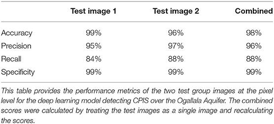
Table 1. Model evaluation metrics.

Even with the differences in imagery resolution used for training, the model performed comparably to the original deployed in Brazil by Saraiva et al. (2020) as evidenced by it achieving the same recall rate and only slightly reduced accuracy and precision scores. Test image 1 had a much larger share of background pixels than test image 2 which accounts for much of the difference between the images in performance metrics. Because these metrics are calculated at the pixel level, they are influenced by the difficulty the model has with accurately predicting the boundaries of the CPIS as shown in the sample image in Figure 1 where the red area is the model's prediction and the yellow area is the ground truth. These dropped pixels lower the accuracy and recall of the model when evaluated at the pixel level. In order to understand how the model performs from a broader perspective, the test images were visually inspected as well. Test image 2 contains 5,186 CPIS, and the model correctly predicted 4,997 of these CPIS giving it a recall rate of about 96% when evaluated at the structure level as seen in Figure 2 which shows the model's output in red.

FIGURE 1

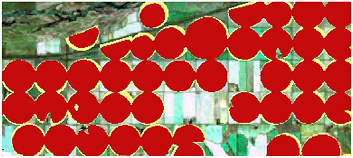
Figure 1. Model output for predicted CPIS from test Image 1. The deep learning model's output (red) superimposed on the manually identified center pivots (yellow). The model is capable of detecting CPIS of varying sizes and shapes as can be seen near the top of the image.

FIGURE 2

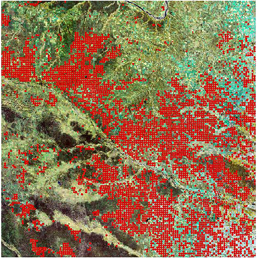
Figure 2. Deep learning model output for test Image 2. This figure shows the predicted CPIS locations (red) from the deep learning model over a 100 × 100 km test image. This image was not used in the training process of the model, so it should be indicative of how the model performs on previously unseen images with environments similar to the training images. As can be seen in the upper right hand side of the figure, the model is able to distinguish farmland irrigated by CPIS from farmland that is irrigated by some other technology.

After the model was trained, satellite imagery covering the entire Ogallala Aquifer was obtained from the same sources for 2008. The model's prediction of CPIS locations is provided in Figure 3 for all of the land overlying the aquifer. The validity of these predictions depends on the environmental factors over the rest of the Ogallala Aquifer being similar enough to those of Nebraska. The test results of the trained model along with the prevalence of CPIS over the Ogallala and the semiarid climate of the region suggest that this assumption holds true.

FIGURE 3

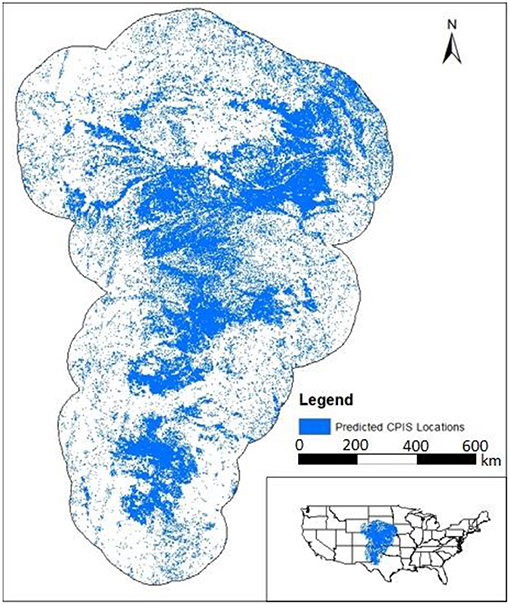
Figure 3. Predicted CPIS in the Ogallala Aquifer region. This figure shows the final product of the deep learning model when used to predict CPIS locations for the Ogallala Aquifer region, including a 100 km buffer zone. Predicted CPIS locations are depicted as blue dots which are largely concentrated in the central Ogallala and become less prevalent in the buffer zone.

Economic Applications

The knowledge of the location and extent of CPIS can improve economic analysis at a variety of scales and applications. Here we demonstrate its importance in a county-level model—a common unit of analysis in agricultural economics—and also discuss other potential uses. In economics many studies have considered irrigation uptake and its effects on farming across the U.S. and the Ogallala specifically (Hornbeck and Pinar, 2014; Edwards and Smith, 2018; Smith and Edwards, 2021). Many have been Kansas specific due to its high-quality data (Hendricks and Peterson, 2012; Pfeiffer and Lin, 2012, 2014; Edwards, 2016; Drysdale and Hendricks, 2018). To get greater geographic coverage and additional outcomes, a popular source of data comes from the USDA Agricultural Census gathered roughly every 5 years back to 1920 and each decade back to 1860. Data is publicly available at the county level and irrigation information has been reported since 1890 (Haines et al., 2018). However, CPIS specific data was only gathered in 1959 and 1969. To illustrate the importance of irrigation technology, we combine the deep learning CPIS data with the USDA data.

Hornbeck and Pinar (2014) demonstrate that irrigation uptake for counties over the Ogallala Aquifer increased dramatically both in absolute terms and relative terms compared to nearby counties not over the aquifer after the arrival of CPIS technology circa 1948. This led to greater production and increased farm values. Other work has shown that not only did average production increase, resilience to drought is greater when counties are over an aquifer even compared to counties with similar irrigation levels but sourcing from surface water (Smith and Edwards, 2021). Neither paper, however, considers the role of the CPIS technology in specifically shaping these relationships. Because our model used data from 2008, we begin with the closest USDA NASS (2009) to provide a few insights.

First, in Figure 4, we show that CPIS is not ubiquitous across the Ogallala region and “irrigated hectares” are not all using the same technology. The scatter plot compares the fraction of the county with irrigated hectares from the census compared to the fraction with CPIS technology from our deep learning model. Using the 45-degree line for reference, many areas had more irrigated hectares than CPIS hectares, meaning that other technologies are deployed, even over the Ogallala Aquifer. However, it also shows that CPIS share can be greater than irrigated share in a given year. Although some of the discrepancy could be related to model error, particularly at lower shares, it is also consistent with other findings that irrigators of groundwater generally (Smith and Edwards, 2021) and over portions of the Ogallala specifically (Deines et al., 2017) are more flexible in reducing and expanding irrigated area than surface water users. In other words, our detection of CPIS captures a measure of irrigation capacity which may or may not be deployed in a given year for reasons related to farm-level decisions.

FIGURE 4

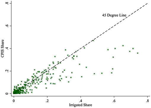
Figure 4. Irrigation share vs. CPIS share, Ogallala. This provides a scatter plot of irrigated share, reported in the 2007 Census, and the CPIS share calculated, from our model, for the Ogallala counties (within 100 km of the aquifer boundary).

Second, we show the positive relationship between center pivots and farm value are stronger than just irrigation and land value over the Ogallala. We regress

$\begin{array}{ll}{Y}_{is}={\gamma }_{1}Ir{r}_{is}+{\gamma }_{2}CPI{S}_{is}+X_{is}+{\theta }_s+{\epsilon }_{is}& (5)\end{array}$

For dependent variables we consider farm value per county hectare and total value of crops sold per county hectare in county i of state s. We take the natural log of both so the coefficient estimates can be interpreted as the percent change of the dependent variable. The coefficients of interest are the γ's on Irr_is (share of county irrigated) and CPIS_is (share of county with a CPIS). The vector X_is includes covariates (and their coefficients) that may also affect crop and farm value: population density, elevation, elevation variation, soil, share within 24 km of a Strahler order 3 or higher stream, 30-year average temperature and precipitation, average wind class, maximum wind class, kilometers of transmission lines, and latitude and longitude. Finally, θ_s is included as a state fixed effect, controlling for similarities of all counties within a given state.

Table 2 shows the results. While counties with an additional 10 percent of irrigated land have 9.79 percent higher farm values on average (column 1), another 10 percent more of CPIS is associated with 13.1 percent more valuable farm land. When both controls are included in the same regression (column 3), the relationship still holds and the effect of CPIS is statistically and economically significantly different from just irrigation alone. Additional results with crop revenue as the dependent variable (columns 4–6) follow similar lines, although the additional value related to CPIS above and beyond irrigation is relatively more for this outcome.

TABLE 2

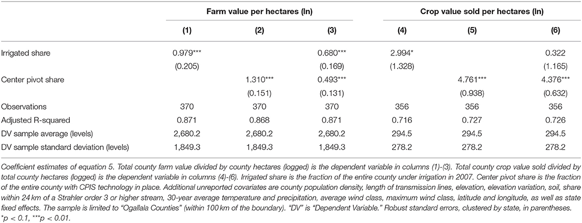
Table 2. Irrigation, farm value and production, 2007.

These results are not causal. They do not claim the CPIS leads to the higher values and it remains plausible that higher productivity, for reasons not captured by the covariates, makes the return on investing in CPIS technology higher. In other words, the higher value could drive more CPIS. The truth of the causality surely lies somewhere between. However, the point is that the irrigation technology information provides additional insights beyond what the simple metric of irrigated area does.

As a third exercise, we consider the resilience irrigation provides agriculture production to various weather anomalies, comparing results for irrigated shares and CPIS shares specifically. The analysis is similar to that in Smith and Edwards (2021) in that it considers the production change within a county under positive and negative deviations from the counties' 100-year temperature and precipitation averages. The analysis encompasses the 15 Agricultural Censuses going back to 1950, once center pivot technology emerged. The baseline weather is “normal” and the coefficient estimates shown in Figure 5 represents the percentage change in crop production (by value) with no irrigation (zero irrigated hectares), for counties' irrigated hectares, and counties' CPIS hectares, both scaled to a one-standard deviation increase in the share of the county irrigated (0.15). Full details are provided in the SI appendix.

FIGURE 5

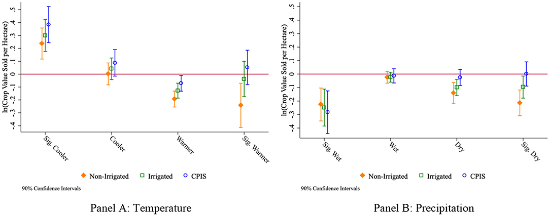
Figure 5. Effect of irrigation on crop revenue resilience. Coefficient estimates of equation SI.1 from the SI Appendix. The dependent variable is the natural log of crop value sold per county hectare from the 1950, 1954, 1959, 1964, 1969, 1974, 1978, 1982, 1987, 1992, 1997, 2002, 2007, 2012, and 2017 Agricultural Censuses. The estimates represent deviations from a county's average relative to normal levels of temperature (A) and precipitation (B). Irrigated and CPIS shares are the fractions of the county irrigated or with CPIS available, respectively, as of 2007. The effect shown is for a one standard deviation increase of irrigated share (0.15). Because “Irrigation” and “CPIS” are not nested, the coefficients come from separate estimations. Year and county fixed effects are included as well as a third-order polynomial of temperature. The sample are the arid counties (west of the 98th meridian) from the “Ogallala counties” (within 100 km of the aquifer boundary).

In Figure 5 we provide the estimated coefficients. The left panel (A) uses temperature as the weather variable. Here, abnormally cool years increase production across the board, but warmer and significantly warmer years reduce baseline production. Irrigation mitigates the losses. Estimates for CPIS indicate a more positive effect in addressing warmer weather, although it is not statistically distinct from irrigation on its own. Resilience to local precipitation shocks is shown in the right panel (B). Here, no matter the irrigation, significantly wetter years hurt production for all counties. Irrigation offsets losses in dry and significantly dry years, but CPIS does even better at maintaining production levels closer to that in normal years.

The upshot of these three exercises is that economic relationships are sensitive to the irrigation technology present and the deep learning model can provide improved inputs for the economic models. Beyond these examples, the deep learning model could be used to develop a panel data set and analyze the adoption of CPIS systems as well as the effects of that adoption. Additionally, these economic models here aggregate data to the county level but the deep learning model outputs a raster and can be deployed at many scales to better characterize economic irrigation decisions (see Smith and Cooley, 2021 for a Public Land Survey System grid example at the square mile, or 2.6 km², scale). Given the relative ease of running the deep learning model, it could pick up on new CPIS systems so that we can better model and understand its adoption and effects on the food-energy-water nexus.

Implications for Hydrologic Modeling

Hydrologic models that include pumping and irrigation are commonly used to assess the effects of agriculture on water availability, particularly groundwater (see e.g., the review by Haacker et al., 2019 and references therein). Such models can be powerful tools for planning and resource management and have grown in scale to include global groundwater use for food production (e.g., Wada et al., 2010; de Graaf et al., 2019) to study economic and environmental limits to pumping. These models all require many input parameters to define the location and extent of irrigated area and pumping wells. As these input data are often not directly available, they are often based on coarser resolution (e.g., county level) information or land cover classification from nation datasets (e.g. Gilbert et al., 2017; Thatch et al., 2020), depletion estimates lumped over major aquifers (e.g., Konikow, 2013), or combined from model simulations and administrative databases (e.g.. Siebert et al., 2010).

As these models grow in size to the national scale and decrease in resolution, these inputs become problematic due to lack of records and inconsistencies across administrative boundaries. As an example, a recent study (Condon and Maxwell, 2019) combined two different datasets (the coarse scale Konikow depletions and the model derived pumping and irrigation from the Wada et al. model simulations) to reconstruct groundwater depletion and ongoing pumping at the national scale. The results of our deep learning model allow for direct input of CPIS into hydrology models, providing a new way to estimate the effects on groundwater pumping. The results of this current work provide an unprecedented, high resolution input dataset for the location of irrigation and pumping wells in the Ogallala Aquifer. The CPIS estimates in Figure 3 were converted to pumping estimates and compared to the groundwater pumping used to drive the Condon and Maxwell (2019) study (Figure 6). The CPIS image was converted to an estimate of groundwater pumping in Kansas based on a detailed study by Pfeiffer and Lin (2014). This study estimated an annual groundwater extraction of 1.995 × 10⁵ m³ (161.73 AF) per center pivot, which can be scaled to an aerial estimate of 1,332 m³. Applying this value to each identified CPIS pixel, we scale up to a 1 km resolution to estimate the location and extent of groundwater pumping in 2008. The result is shown in Figure 6A. The Condon and Maxwell (2019) study combined two long term groundwater depletion and pumping estimates into one product. This product resulted from combining the Wada et al. (2010) pumping estimates at a 6-min (~11 km) native resolution and the Konikow (2013) estimate of total aquifer depletions, is plotted in Figure 6B and represents an estimate of average pumping per year from 1960 to 2010.

FIGURE 6

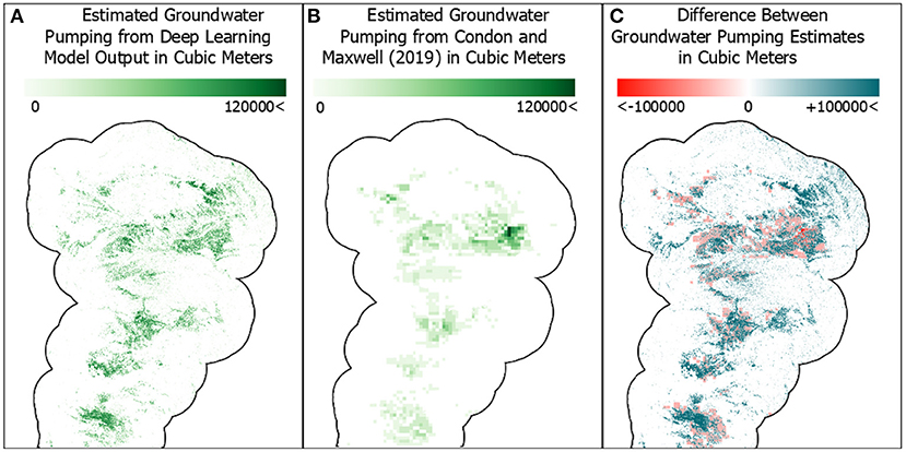
Figure 6. Comparison of groundwater pumping estimates in the Ogallala Aquifer. The maps in all panels are in 1 × 1 km resolution which involved resampling the underlying data from 30 × 30 m resolution for the deep learning model's output and 11 × 11 km resolution for the Condon and Maxwell (2019) data. The map in (C) shows where the estimates in (A) are less than the estimates in (B) in red while the areas marked in blue show where the estimates in (A) are greater than the estimates in (B). Areas with a high concentration of CPIS along with the surrounding land show the most remarkable differences between the two approaches.

Several things are striking about these results. First is the dramatic increase in resolution the ML-based approach provides. Second is the general similarity between the two images; both images show similar patterns in pumping location, despite being derived using very different approaches. Third, and perhaps most importantly, is the difference in overall pumping amount shown in Figure 6C. The ML-based approach estimates a much larger pumping volume than the Condon and Maxwell (2019) estimate. A summation of the two pumping estimates quantifies this difference: the Condon and Maxwell (2019) estimates 6.68 × 10⁹ m³/y (5.42 × 10⁶ AF/y) of total pumping, while the ML-based approach presented here estimates 1.96 × 10¹⁰ m³/y (1.59 × 10⁷ AF/y) of pumping in 2008.

This dramatic (almost three times greater) estimate is likely due to several reasons. First, pumping is likely to have increased during the 1960–2010 time period; the average rate over a half century likely underestimates the rate in 2008. Second, the estimates of pumping in the Condon and Maxwell (2019) dataset rely heavily on the Wada et al. (2010) model simulations which are global in extent and driven to a large degree by water demand. These source data may be subject to uncertainty and are at a coarser resolution than the current study, which might further underestimate the magnitude of pumping. Lastly, the approach used to convert the CPIS density to groundwater pumping is well-validated in Kansas, but may have uncertainties when applied to the entire Ogallala. Nevertheless, these ML-based results suggest an underestimation of pumping in the Great Plains region by prior studies and offer an additional avenue for estimating these quantities.

In addition to the dramatic differences in the estimates of annual pumping rate, the results shown in Figure 6 may be directly input into models used for planning (e.g., Haacker et al., 2019) to improve their representation of agricultural processes. Additionally, the methodology used here can be applied over time to understand the expansion of groundwater pumping and depletion.

Conclusion

We have refined and described a deep learning model that identifies CPIS technology across the Ogallala Aquifer region. The model is meant to overcome the lack of consistent spatial data on irrigation technology adoption across jurisdictions. Manually identifying CPIS from aerial or satellite imagery is a time-consuming and tedious process that may be cheaply replaced by utilizing the open-source deep learning model presented in this paper. It utilizes readily available satellite images and a combination of Google Colab Pro and Google Earth Engine that avoids the need for a GPU cluster or supercomputer, yet trains relatively quickly and performs well on a 30-m spatial resolution.

Furthermore, we provide evidence that CPIS are economically distinct from other forms of irrigation technology and their locations are a useful input to hydrologic models involving groundwater pumping. The final raster produced by the deep learning model used in this paper can provide a valuable input to future economic and hydrologic research concerning the Ogallala Aquifer. The model itself can be applied to identify CPIS in other instances where the climate variables are similar enough to the original dataset. Most immediately, this would be the Ogallala itself in different time periods to explore the dynamic changes in irrigation technology.

In order to keep within the confines of the processing power offered by Google Colab Pro, the model was only trained on data from Nebraska. However, there are a few other sets of manually identified CPIS data (e.g. ISWS, 2015; USGS, 2021) that could be incorporated into the model's training to allow it to be even more generalizable and more accurate. The model, as is, struggles in more humid regions because the boundary between land irrigated by a CPIS and the surrounding area is less clear, yet the technology is increasingly deployed as a climate resiliency tool in humid regions like Illinois (Cooley and Smith, 2021). This shortcoming can be circumvented by drawing on times of major drought when the iconic circular pattern of the CPIS is more distinguishable (e.g., Cooley and Smith, 2021), but additional refinement of the model could improve detection under a wider range of climactic conditions, leading to better temporal and spatial coverage. Finally, the model could also be altered to identify irrigation technologies other than CPIS. While all of these would require more costly and time-consuming methods to run, it could also provide an even more valuable resource to economists and hydrologists making it a useful endeavor for future research.

Data Availability Statement

The raw data supporting the conclusions of this article will be made available by the authors, without undue reservation.

Author Contributions

All authors contributed to the conception and design of the study. DC gathered and organized the data, implemented the deep learning model, and wrote the initial draft. SS performed the data analysis. All authors assisted with interpretation of results, wrote sections of the paper, contributed to manuscript revisions, and approved the submitted version.

Conflict of Interest

The authors declare that the research was conducted in the absence of any commercial or financial relationships that could be construed as a potential conflict of interest.

Publisher's Note

All claims expressed in this article are solely those of the authors and do not necessarily represent those of their affiliated organizations, or those of the publisher, the editors and the reviewers. Any product that may be evaluated in this article, or claim that may be made by its manufacturer, is not guaranteed or endorsed by the publisher.

Acknowledgments

We are grateful for financial support from NSF/USDA (INFEWS Grant #67020-30130).

References

Bierkens, M. F. P., and Wada, Y. (2019). Non-renewable groundwater use and groundwater depletion: a review. Environ. Res. Lett. 14:063002. doi: 10.1088/1748-9326/ab1a5f

CrossRef Full Text | Google Scholar

Condon, L. E., and Maxwell, R. M. (2019). Simulating the sensitivity of evapotranspiration and streamflow to large-scale groundwater depletion. Sci. Adv. 5:aav4574. doi: 10.1126/sciadv.aav4574

PubMed Abstract | CrossRef Full Text | Google Scholar

Cooley, D., and Smith, S. M. (2021). Benefits of Investing in Center Pivot Irrigation Systems in Humid Regions: A Case Study of Illinois. Golden: Working Paper.

de Graaf, I. E. M., Gleeson, T., and van Beek, L. P. H. (2019). Environmental flow limits to global groundwater pumping. Nature 574, 90–94. doi: 10.1038/s41586-019-1594-4

PubMed Abstract | CrossRef Full Text | Google Scholar

Deines, J. M., Kendall, A. D., Crowley, M. A., Rapp, J., Cardille, J. A., and Hyndman, D. W. (2019). Mapping three decades of annual irrigation across the US high plains aquifer using landsat and google earth engine. Remote Sensing Environ. 233:111400. doi: 10.1016/j.rse.2019.111400

CrossRef Full Text | Google Scholar

Deines, J. M., Kendall, A. D., and Hyndman, D. W. (2017). Annual irrigation dynamics in the U.S. Northern high plains derived from landsat satellite data. Geophys. Res. Lett. 44, 9350–9360. doi: 10.1002/2017GL074071

PubMed Abstract | CrossRef Full Text | Google Scholar

Dieter, C. A., Maupin, M. A., Caldwell, R. R., Harris, M. A., Ivahnenko, T. I., Lovelace, J. K., et al. (2018). Estimated use of water in the United States in 2015. USGS 5:1441. doi: 10.3133/cir1441

CrossRef Full Text | Google Scholar

Drysdale, K. M., and Hendricks, N. P. (2018). Adaptation to an irrigation water restriction imposed through local governance. J. Environ. Econ. Manage. 91, 150–165. doi: 10.1016/j.jeem.2018.08.002

CrossRef Full Text | Google Scholar

Edwards, E. C.. (2016). What lies beneath? Aquifer heterogeneity and the economics of collective action. J. Assoc. Environ. Resource Econ. 3, 453–491. doi: 10.1086/685389

CrossRef Full Text | Google Scholar

Edwards, E. C., and Smith, S. M. (2018). The role of irrigation in the development of agriculture in the United States. J. Econ. Hist. 78:608. doi: 10.1017/S0022050718000608

PubMed Abstract | CrossRef Full Text | Google Scholar

Gilbert, J. M., Maxwell, R. M., and Gochis, D. J. (2017). Effects of water-table configuration on the planetary boundary layer over the San Joaquin River Watershed, California. J. Hydrometeorol. 18, 1471–88. doi: 10.1175/JHM-D-16-0134.1

CrossRef Full Text | Google Scholar

Goodfellow, I., Bengio, Y., and Courville, A. (2016). Deep Learning. Cambridge, MA: MIT Press.

Google Scholar

Gowda, P., Steiner, J. L., Olson, C., Boggess, M., Farrigan, T., and Grusak, M. A. (2018). Chapter 10: Agriculture and Rural Communities. Washington, DC: Fourth National Climate Assessment.

PubMed Abstract | Google Scholar

Haacker, E. M. K., Kendall, A. D., and Hyndman, D. W. (2016). Water level declines in the high plains aquifer: predevelopment to resource senescence. Groundwater 54, 231–242. doi: 10.1111/gwat.12350

PubMed Abstract | CrossRef Full Text | Google Scholar

Haacker, E. M. K., Sharda, V., Cano, A. M., Hrozencik, R. A., Núñez, A., Zambreski, Z., et al. (2019). Transition pathways to sustainable agricultural water management: a review of integrated modeling approaches. J. Am. Water Res. 55, 6–23. doi: 10.1111/1752-1688.12722

CrossRef Full Text | Google Scholar

Haines, M., Fishback, P., and Rhode, P. (2018). United States Agriculture Data, 1840-2012. Ann Arbor: Inter-University Consortium for Political and Social Research.

Google Scholar

Hendricks, N. P., and Peterson, J. M. (2012). Fixed Effects estimation of the intensive and extensive margins of irrigation water demand. J. Agri. Res. Econ. 37, 1–19. doi: 10.22004/ag.econ.122312

CrossRef Full Text | Google Scholar

Hornbeck, R., and Pinar, K. (2014). The historically evolving impact of the ogallala aquifer: agricultural adaptation to groundwater and drought. Am. Econ. J. Appl. Econ. 6, 190–219. doi: 10.1257/app.6.1.190

CrossRef Full Text | Google Scholar

Hrozencik, A.. (2019). Irrigation and Water Use. Economic Research Service USDA. Available online at: www.ers.usda.gov/topics/farm-practices-management/irrigation-water-use/ (accessed September 23, 2019).

Google Scholar

ISWS (2015). Illinois State Water Survey: Illinois Center Pivot Irrigation. Illinois Geospatial Data Clearinghouse. Available online at: http://clearinghouse.isgs.illinois.edu/data/hydrology/illinois-center-pivot-irrigation (accessed January 12, 2021).

Google Scholar

Konikow, L. F.. (2013). Groundwater Depletion in the United States (1900-2008). U.S. Geological Survey Scientific Investigations Report 63. doi: 10.3133/sir20135079

PubMed Abstract | CrossRef Full Text | Google Scholar

Pfeiffer, L., and Lin, C. Y. C. (2012). Groundwater pumping and spatial externalities in agriculture. J. Environ. Econ. Manage. 64, 16–30. doi: 10.1016/j.jeem.2012.03.003

CrossRef Full Text | Google Scholar

Pfeiffer, L., and Lin, C. Y. C. (2014). Does efficient irrigation technology lead to reduced groundwater extraction? Empirical evidence. J. Environ. Econ. Manage. 67, 189–208. doi: 10.1016/j.jeem.2013.12.002

CrossRef Full Text | Google Scholar

PRISM Climate Group (2004). PRISM Climate Data. Oregon State University.

Saraiva, M., Protas, E., Salgado, M., and Souza, C. (2020). Automatic mapping of center pivot irrigation systems from satellite images using deep learning. Remote Sensing 12:558. doi: 10.3390/rs12030558

CrossRef Full Text | Google Scholar

Schmidhuber, J.. (2015). Deep learning in neural networks: an overview. Neural Netw. 61, 85–117. doi: 10.1016/j.neunet.2014.09.003

PubMed Abstract | CrossRef Full Text | Google Scholar

Siebert, S., Burke, J., Faures, J. M., Frenken, K., Hoogeveen, J., Döll, P., et al. (2010). Groundwater Use for Irrigation - a Global Inventory. Hydrol. Earth Syst. Sci. 14, 1863–1880. doi: 10.5194/hess-14-1863-2010

CrossRef Full Text | Google Scholar

Smith, S. M., and Cooley, D. (2021). Water and Wind: Tradeoffs of Irrigation and Clean Energy. Golden: Working Paper.

Google Scholar

Smith, S. M., and Edwards, E. C. (2021). Water storage and agricultural resilience to drought: historical evidence of the capacity and institutional limits in the United States. Environ. Res. Lett. 16:358. doi: 10.1088/1748-9326/ac358a

CrossRef Full Text | Google Scholar

State of Nebrasksa Open Data (2019). 2005 Center Pivots in the Central Platte River Basin. Available online at: https://www.nebraskamap.gov/datasets/8e7b99d90da84c82889e00ba8f90ef41_0?geometry=-108.327%2C40.017%2C-90.936%2C42.898 (accessed April 18, 2019).

Tang, J., Arvor, D., Corpetti, T., and Tang, P. (2020). Pvanet-hough: detection and lcation of center pivot irrigation systems from sentinel-2 images. ISPRS Ann. Photogrammetry Remote Sens. Spatial Inform. Sci. 3, 559–564. doi: 10.5194/isprs-annals-V-3-2020-559-2020

CrossRef Full Text | Google Scholar

Tang, J., Arvor, D., Corpetti, T., and Tang, P. (2021). Mapping center pivot irrigation systems in the southern amazon from sentinel-2 images. Water 13:298. doi: 10.3390/w13030298

CrossRef Full Text | Google Scholar

Thatch, L. M., Gilbert, J. M., and Maxwell, R. M. (2020). Integrated hydrologic modeling to untangle the impacts of water management during drought. Groundwater 58, 377–391. doi: 10.1111/gwat.12995

PubMed Abstract | CrossRef Full Text | Google Scholar

USDA NASS (2009). Census of Agriculture: 2007. Available online at: https://www.nass.usda.gov/Publications/AgCensus/2007/ (accessed November 29, 2021).

USDA NASS (2018). Census of Agriculture: 2018 Irrigation and Water Management Survey. Available online at: https://www.nass.usda.gov/Publications/AgCensus/2017/Online_Resources/Farm_and_Ranch_Irrigation_Survey/index.php (accessed September 16, 2021).

USGS (2013). Groundwater Decline and Depletion. USGS. Available online at: https://www.usgs.gov/special-topic/water-science-school/science/groundwater-decline-and-depletion?qt-science_center_objects=0#qt-science_center_objects (accessed September 16, 2021).

USGS (2021). Geospatial Compilation and Digital Map of Center-Pivot Irrigated Areas in the Mid-Adlantic Region, United States. FirstMap. Available online at: https://firstmap.gis.delaware.gov/arcgis/rest/services/Hydrology/DE_Pivot_Irrigation/MapServer (accessed January 21, 2021).

Google Scholar

Valencia, O. M. L., Johansen, K., Solorio, B. J. L. A., Li, T., Houborg, R., Malbeteau, Y., et al. (2020). Mapping groundwater abstractions from irrigated agriculture: big data, inverse modeling, and a satellite-model fusion approach. Hydrol. Earth Syst. Sci. 2020, 5251–5277. doi: 10.5194/hess-24-5251-2020

CrossRef Full Text | Google Scholar

Wada, Y., van Beek, L. P. H., van Kempen, C. M., Reckman, J. W. T. M., Vasak, S., and Bierkens, M. F. P. (2010). Global depletion of groundwater resources. Geophy. Res. Lett. 37:L20402. doi: 10.1029/2010GL044571

CrossRef Full Text | Google Scholar

Zhang, C., Yue, P., Di, L., and Wu, Z. (2018). Automatic identification of center pivot irrigation systems from landsat images using convolutional neural networks. MDPI Agri. Spec. Issue. 8:147. doi: 10.3390/agriculture8100147

CrossRef Full Text | Google Scholar

SI Appendix

The regression framework for resilience is as follows:

$\begin{array}{l}{Y}_{it}={\displaystyle \sum _{j=-2}^2}{\alpha }^j·Bi{n}_{it}^j+{\displaystyle \sum _{j=-2}^2}{\beta }^j·{Ir{r}_i\times Bin}_{it}^j+f(tem{p}_{it})\\ +{\tau }_t+{\gamma }_i+u_{it}(SI.1)\end{array}$

Y_it is the natural log of total farmland value (buildings and land) in county i in year t divided by total county area or the total crop value in county i in year t divided by total county area. County borders are fixed to their 1910 boundaries and USDA census data is reweighted under the assumption of spatially uniform distribution. $Bi{n}_{it}^j$ is a series of indicators of weather indicators for where in the county-specific weather distribution for the growing season (April-September) falls in its standardized distribution built from annual data from 1900 to 2017 (PRISM Climate Group, 2004). The omitted bin is “normal”, taken as -0.5 to 0.5 standard deviations. Higher bin numbers are more drought oriented with bin 1 indicating the year is 0.5 to 1.5 standard deviations less rain (or higher temperatures) and bin 2 indicates the county year observation is greater than 1.5 standard deviations of less rain (or higher temperatures). Bins -1 and -2 are similarly defined as wetter and cooler years. Irr_i is a continuous measure of share of the county irrigated, either irrigated hectares reported in the 2007 census or the share of CPIS systems from our deep learning model. α^j coefficients provide the baseline with no irrigation and the β^j estimates how an irrigated county performs differently from no irrigation. The figure in the text provide α^j for the baseline and α^j + β^j × 0.145, where 0.145 is one standard deviation of the irrigated share in the sample. f(temp_it) is a flexible polynomial for the temperature (a third order polynomial). τ_t is a series of year fixed effects to absorb macroeconomic conditions and price variation among other elements that vary equally for all counties in that year. γ_i is a series of county level fixed effects to absorb any time-invariant features of the county that affects its production. On net, the estimates use variation from the county average and the annual average of production and weather shock. The sample is limited to counties within 100 km of the outer border of the Ogallala Aquifer and west of the 98^th Meridian. Sample includes census observations from 1950, 1954, 1959, 1964, 1969, 1974, 1978, 1982, 1987, 1992, 1997, 2002, 2007, 2012, and 2017.