Robust Behrens–Fisher Statistic Based on Trimmed Means and Its Usefulness in Analyzing High-Throughput Data

In the context of high-throughput data, the differences in continuous markers between two groups are usually assessed by ordering the p-values obtained from the two-sample pooled t-test or Wilcoxon–Mann–Whitney test and choosing a stringent cutoff such as 10^–8 to control the family-wise error rate $\left(FWER\right)$ or false discovery rate $\left(FDR\right).$ All markers with p-values below the cutoff are declared to be significantly associated with the phenotype. This inherently assumes that the test procedure provides valid type I error estimates in extreme tails of the null distribution. The aforementioned tests assume homoscedasticity in the two groups, and the t-test further assumes underlying distributions to be normally distributed. Cao et al. (Biometrika, 2013, 100, 495–502) have shown that in the context of multiple hypotheses testing the approach based on $FDR$ may not be valid under non-normality and/or heteroscedasticity. Therefore, having a test statistic that is robust to these violations is needed. In this study, we propose a robust analog of Behrens–Fisher statistic based on trimmed means, conduct an extensive simulation study to compare its performance with other competing approaches, and demonstrate its usefulness by applying it to DNA methylation data used by Teschendorff et al. (Genome Res., 2010, 20, 440–446). An R program to implement the proposed method is provided in the Supplementary Material.

1 Introduction

In the context of genetic analysis, it is quite common to compare hundreds of thousands of genetic features such as gene expressions or DNA methylations between cases and controls. The well-known two-sample t-test or its robust analog Wilcoxon rank sum test has been commonly utilized to obtain p-values for comparing genetic features between the two groups at each locus. These p-values are then ordered and chosen to control the family-wise error rate $\left(FWER\right)$ or false discovery rate $\left(FDR\right)$ based on a cutoff; all p-values below that threshold are declared to have significantly different genetic features between two groups, for example, see Hochberg and Tamhane (1987), Storey (2002), and Benjamini and Yekutieli (2007). The validity of this approach is based on two underlying assumptions: 1) the p-values under the null hypothesis would be uniformly distributed, whereas the p-values under alternative hypothesis would tend to have values closer to 0; 2) the null distribution of the test statistic is well controlled even for stringent levels of $\alpha .$ However, Robins et al., (2000) have shown that the p-values will be uniformly distributed under $H_0$ (null model) only when the test statistic $T$ generating the p-values consists of a single distribution. On the other hand, if the null distribution of $T$ depends on the nuisance parameters, then the p-values will not be uniformly distributed.

When a study involves testing the differences between several thousands of genes between cases and controls, then it may be reasonable to assume that the sample size would be fixed for all comparisons. However, the p-values for comparing a gene expression profile between the two groups would still be affected by the effect size (standardized difference in the mean expression levels), underlying distributional assumptions (usually normality), and inequality of the variances for the two groups. In the context of a multiple-hypotheses setting, it is clear that $FDR\left(u\right),$ where $u$ denotes the cutoff based on the test statistic, must be an increasing function in $u$, and Cao et al. (2013) have shown that this monotonicity assumption could be violated and could lead to misleading results when the underlying distributions are not normal and/or have significantly different variances.

In the parametric setting, it is well known that the pooled two-sample t-test is optimal for comparing the two means when the underlying distributions are normal and have equal variances. When the variances are not equal, then one uses the Behrens–Fisher statistic with the Satterthwaite approximation; see Welch (1937) and Satterthwaite (1946).

However, it is also well known that these assumptions are rarely met in practice, and an alternative is to use non-parametric approaches that impose fewer conditions on the underlying distributions. For the two-sample location problem, one is often interested in comparing the medians of the two populations, and the widely used Wilcoxon–Mann–Whitney (WMW) test is distribution-free, if the two distributions are continuous and have the same shape. Pratt (1964) has shown that the test does not maintain type I error if the variances are different. Fligner and Policello (1981) proposed a modified WMW statistic for unequal variances but assumed the two populations to be symmetric. Brunner and Munzel (2000) and Neubert and Brunner (2007) further extended the non-parametric statistics to more general situations by further relaxing the underlying assumptions.

In general, it is well recognized, for example, Hampel et al. (1986) showed that the parametric tests would be optimal, that is, they would be valid and have the optimal power, when the underlying assumptions are satisfied. On the other extreme are the non-parametric tests that have minimal assumptions on the underlying distribution, but a price is paid in terms of loss of power. However, when there are modest departures from the target family (usually normal), robust methods serve as a viable alternative as they provide significant gain in power while maintaining the type I error control. In the context of the two-sample problem, assuming the underlying distributions to be in the neighborhood of the normal family with equal variances, Srivastava et al. (1992) and Mudholkar et al. (1991) have proposed robust test procedures based on L-statistics. In particular, the approach based on trimmed means, which is based on the concept of trimming the extreme observations, seems appealing and has shown better operating characteristics particularly for the distributions that are heavier tailed than normal.

It would be a daunting task to test the underlying distributional assumption and the homogeneity of variances at each locus and then use the appropriate test statistic based on the results of those tests. Even if one performed that, one will have to account for the increased number of tests being performed and the conditional nature of the p-values in the second stage. Pounds and Rai (2009) adopted the concept of an assumption adequacy averaging approach, which incorporates an assessment of the assumption of normality and weighs the results of the two alternative approaches based on whether the assumption of normality is satisfied or not. However, their approach does not extend to the situations where the assumptions of normality and homoscedasticity may be violated simultaneously.

The hallmarks of a “good” robust procedure should be that which is able to control the type I error rate and provide significant gain in power when the underlying assumptions are violated. Also, it should be able to maintain the type I error control with minimal loss in power when the underlying assumptions hold. The literature is filled with robust test procedures proposed for comparing two populations, and it is worthwhile to note that majority of them assess the type I error control at the traditional level of $\alpha$ = 0.05, with few exceptions, for example, see Lee (1995). Fagerland and Sandvik (2009) compared the robustness of five two-sample location tests for skewed distributions and concluded that the tests conducted at $\alpha =0.01$ were less robust than those conducted at $\alpha =\mathrm{0.05.}$ However, it may be noted that in the context of testing multiple hypotheses or in the context of controlling $FWER$, it is essential that the performance of a test procedure be evaluated at more stringent type I error rates such as 0.001, 0.0001, or even lower as we are looking for p-values in the tail of the distribution. It is also seen that in the context of designing genomic studies, often the sample size justification uses more stringent level of $\alpha$ such as 10^–4 or 10^–5, as seen in Chow et al. (2008) and Kang et al. (2009). It is not difficult to visualize that, in this context, a test that is valid (could be somewhat conservative without significant loss in power) at stringent levels of $\alpha$ is likely to give fewer false positives than the tests that are unable to control the type I error. Thus, in conducting genetic analysis, one must ensure that the test statistic used is not only robust to the violations of the underlying model assumptions but also exhibits good operating characteristics even at stringent levels of type I error.

In this study, we propose a robust analog of the Behrens–Fisher statistic based on trimmed means that is robust to the violations of underlying assumptions of normality and homogeneity. We use the asymptotic normality of trimmed means, derived by Huber (1970), to obtain the asymptotic distribution of the proposed test statistic. Then, using the first two moments of the proposed test statistics and regression methods, we obtain finite sample approximations to make the statistics useful in small sample sizes. The proposed statistic provides for a robust alternative for comparing two distributions that may not be normal and may be heteroscedastic. It is interesting to note that the proposed test statistic has the best performance for skewed distributions as well. However, in the context of high-throughput studies, the results based on the p-value approach will also be affected by the correlations among the test statistics by virtue of the correlation among genes. In this development, we focus our attention on developing a test statistic that will provide valid p-values when the assumptions of normality and homoscedasticity are violated with the understanding that one could use the approaches described in Benjamini and Yekutieli (2007) or Sun and Cai (2009) to conduct inference with correlated p-values. In Section 2, we provide the details of the motivating example. In Section 3, the background information regarding trimmed means and their asymptotic properties are discussed. In Section 4, a brief account of the Behrens–Fisher statistic for two samples is provided. In Section 5, we propose the new test statistic and obtain null distribution approximations for the proposed test statistic for finite samples. In Section 6, the details of the simulation study to evaluate the performance of the proposed test statistic in terms of type I error control and power properties and its comparison with the existing approaches are provided. In Section 7, the usefulness of the proposed test procedure is demonstrated by applying it to the DNA methylation data. Section 8 is dedicated to discussions and miscellaneous comments.

2 Motivating Example

Teschendorff et al., (2010) conducted a study to investigate the mechanism of diabetic nephropathy by comparing 27580 markers from a genome-wide methylation array between cases and controls. These data were submitted by the authors to the NCBI Gene Expression Omnibus (http://www.ncbi.nlm.nih.gov/geo) under accession nos. GSE20067 and can be easily downloaded. There were 97 cases who had type 1 diabetes (T1D) and nephropathy and 98 controls who had T1D but with no evidence of renal disease. The purpose of this study was to identify the markers that would be differentially expressed between the two groups. Cao et al. (2013) used the two-sample t-test and converted them to p-values to identify the proportions of DNA methylations that were different between the two groups. They further showed that the monotonicity assumption required for the validity of the $FDR$-based approach was violated when the underlying assumption of normality and/or homoscedasticity underlying the two-sample t-test did not hold.

Cao et al. (2013) used the raw proportions of methylation which range between 0 and 100%. However, in practice, the logit transformation is often used before applying any test procedure. The benefit of using this transformation is that it transforms the proportions on a scale that ranges from −∞ to ∞ and possibly achieves variance stabilization; see Box (1953). We checked the assumption of normality in cases and controls and equality of variances between the two groups for all markers using Shapiro and Wilk (1965) and the F-test (Box, 1953) at different significance levels on the raw and logit-transformed methylation data. The results for the logit transformation (raw) are reported, and the results for the raw data were slightly worse.

At the conventional level of $\alpha =0.05,$ there were 88% (92%) of markers that failed the normality test in either cases or controls or had unequal variances between cases and controls, and 30% (46%) of markers failed the normality test for both cases and control and also failed the equal variance test between them. At a more stringent level of $\alpha ={10}^{-4}$, 68% (78%) of the markers failed the normality test in either cases or controls or had unequal variances, and 4% (13%) of the markers failed the normality test for both cases and controls and had unequal variance.

Thus, it is obvious that the assumption of normality and/or equality of variance, in general, is questionable, and robust methods that are robust to such violations should be used. In the following section, we provide the background of the trimmed means and their asymptotic distribution.

3 Trimmed Means and Asymptotic Results

3.1 Trimmed Means

In the univariate case for one sample problem, let $X_1<X_2<\dots <X_n$ be the order statistics of a random sample from a location scale population with the symmetric distribution function $F((x-\theta )/\sigma ).$ For an integer, $g<n$ denotes $\delta -$ trimmed mean, $\delta =g/n,$ by the following equation:

$\tilde{X}=\left(X_{g+1}+\dots +X_{n-g}\right)/\left(n-2g\right),(1)$

where $g$ is the number of observations trimmed from each end. Tukey and McLaughlin (1963) were the first to propose a robust analog of Student’s $t$-test by studentizing given by:

$\tilde{t}=\left(\tilde{X}-\theta \right)/{\tilde{s}}_{TM},(2)$

where

${\tilde{s}}_{TM}^2=\left[(g+1){(X_{g+1}-\tilde{X})}^2+{(X_{g+2}-\tilde{X})}^2+\cdots +(g+1){(X_{n-g}-\tilde{X})}^2\right]/h(h-1),(3)$

is the Winsorized variance, and $h=(n-2g)$ represents the “effective number of observations” obtained by trimming $g$ observations from each end of the ordered observations. They proposed to approximate the null distribution of $\tilde{t}$ by Student’s $t$ distribution with $(h-1)$ degrees of freedom $\left(df\right).$

3.2 Asymptotic Results

Huber (1970) justified the studentization in light of the asymptotic normal distribution of the trimmed means. Specifically, he showed that when the underlying distribution $F$ is symmetric, continuous with mean $\theta$, and variance ${\sigma }^2$ and strictly increasing at points $\pm$ξ, then asymptotically $n\to \infty$:

$\sqrt{n}\left(\tilde{X}-\theta \right)\to N\left(0,{\sigma }^2\left(\delta \right)\right),(4)$

where $\delta =F(-{\xi }_{\delta })$ is the limit of the fraction $g/n$, and

${\sigma }^2\left(\delta \right)=\left[{\displaystyle \underset{-{\xi }_{\delta }}{\overset{{\xi }_{\delta }}{\int }}{x}^{2}dF}+2\delta {\xi }_{\delta }^2\right]/{\left(1-2\delta \right)}^2=b^2\left(\delta \right){\sigma }^2,(5)$

It may be noted that ${\sigma }^2\left(\delta \right)$ is nothing but a function in $\delta$ multiplied by ${\sigma }^2$ that can be explicitly evaluated for a given $F.$ Huber also showed that as $n\to \infty$, then:

$\sqrt{n-1}\left({\tilde{s}}^2-b^2\left(\delta \right){\sigma }^2\right)\to N\left(0,R^2\left(\delta \right){\sigma }^4\right),(6)$

where ${\tilde{s}}^2=\left[(g+1){(X_{g+1}-\tilde{X})}^2+{(X_{g+2}-\tilde{X})}^2+\cdots +(g+1){(X_{n-g}-\tilde{X})}^2\right]/n{(1-2\delta )}^2,$ and $R^2\left(\delta \right)$ can be written as follows:

$R^2\left(\delta \right){\left(1-2\delta \right)}^4{\sigma }^4={{\displaystyle \underset{-{\xi }_{\delta }}{\overset{{\xi }_{\delta }}{\int }}{x}^{4}dF+2\delta \left({\xi }_{\delta }^2+\frac{2\delta {\xi }_{\delta }}{f\left({\xi }_{\delta }\right)}\right)}}^2-{\left[{\displaystyle \underset{-{\xi }_{\delta }}{\overset{{\xi }_{\delta }}{\int }}{x}^{2}dF+}2\delta \left({\xi }_{\delta }^2+\frac{2\delta {\xi }_{\delta }}{f\left({\xi }_{\delta }\right)}\right)\right]}^2.$

Now, if we fix the distribution $F=\Phi ,$ where $\Phi$ represents the normal cumulative distribution function ($cdf$), then Eqs. 4, 6 can be written as follows:

$\sqrt{n}\left(\tilde{X}-\theta \right)\to N\left(0,b_{\mathrm{\Phi }}^2\left(\delta \right){\sigma }^2\right),(7)$

$\sqrt{n-1}\left({\tilde{s}}^2-b_{\mathrm{\Phi }}^2\left(\delta \right){\sigma }^2\right)\to N\left(0,R_{\mathrm{\Phi }}^2\left(\delta \right){\sigma }^4\right),(8)$

where $b_{\Phi }^2\left(\delta \right)$ and $R_{\Phi }^2\left(\delta \right)$ are functions of $\delta$ alone and relatively complex expressions, but they can be very accurately approximated by cubic polynomials. We computed these expressions over a fine grid of $\delta$ from 0 to 0.25, with a step size of 0.01, and used regression methods to find the best polynomial fits. We approximated the functions $b_{\Phi }^2\left(\delta \right)$ and $w_{\Phi }^{\ast }\left(\delta \right)=b_{\Phi }^4\left(\delta \right)/R_{\Phi }^2\left(\delta \right),$ since $R_{\Phi }^2\left(\delta \right)$ appears only indirectly in calculation through $w_{\Phi }^{\ast }\left(\delta \right)$. Hence, we have:

$b_{\mathrm{\Phi }}^2\left(\delta \right)\approx 1+0.48\delta +1.21{\delta }^2,(9)$

$w_{\Phi }\left(\delta \right)=\left(n-1\right)w_{\mathrm{\Phi }}^{\ast }\left(\delta \right)=\left(n-1\right)b_{\mathrm{\Phi }}^4\left(\delta \right)/R_{\mathrm{\Phi }}^2\left(\delta \right)\approx \left(n-1\right)\left(0.5-1.62\delta +1.91{\delta }^2-1.85{\delta }^3\right).(10)$

Using the aforementioned asymptotic theory, Mudholkar et al. (1991) refined the approximation for one-sample trimmed $t$-test and proposed a two-sample pooled trimmed $t$ statistic as a robust analog of the two-sample pooled $t$-test. Now, we provide a brief account of the Behrens–Fisher statistic.

4 Two-Sample Behrens–Fisher Trimmed $\mathit{t}$ Statistic

In the univariate setting for the two-sample problem, let $X_{11}<X_{12}<\dots <X_{1n_1}$ and $X_{21}<X_{22}<\dots <X_{2n_2}$ be the order statistics from two random samples from a location/scale population with a symmetric distribution function $F_i((x-{\theta }_i)/{\sigma }_i)$ for $i=\mathrm{1,2},$ respectively. Under the assumption of normality, $F=\Phi$, the well-known Behrens–Fisher statistic is:

$t_{BF}=\left[\left({\overline{X}}_1-{\overline{X}}_2\right)-\left({\theta }_1-{\theta }_2\right)\right]/\sqrt{s_1^2/n_1+s_2^2/n_2},(11)$

where $s_1^2$ and $s_2^2$ are the sample variances and estimates ${\sigma }_1^2$ and ${\sigma }_2^2,$ respectively. Now, let $R={\sigma }_1^2/{\sigma }_2^2,$ $C=({\sigma }_1^2/n_1)/({\sigma }_1^2/n_1+{\sigma }_2^2/n_2),$ and $f_i=(n_i-1)$ for $i=\mathrm{1,2},$ then it is well known that the rejection region is a function of $R$ and $C$, and many test procedures to conduct the test have been proposed, for example, see Welch (1937, 1947, 1949), Satterthwaite (1946), Lee and Gurland (1975), Cochran and Cox (1950), Wald (1955), and Pagurova (1968). However, the most commonly implemented test procedure is due to Satterthwaite, which approximates the distribution of the Behrens–Fisher statistic in (11) with a $t$-distribution with $\widehat{f}$ degrees of freedom $\left(df\right),$ given by:

$\frac{1}{\widehat{f}}=\frac{{\widehat{C}}^2}{f_1}+\frac{{\left(1-\widehat{C}\right)}^2}{f_2},(12)$

where $\widehat{C}$ is obtained by substituting $s_i^2,$ the sample variance in place of ${\sigma }_i^2,$ where $i=\mathrm{1,2}$. Now, utilizing the background information presented in Sections 3, 4, we present the derivation of the robust Behrens–Fisher statistic.

5 Trimmed $\mathit{t}$ Statistic and its Null Distribution

5.1 Trimmed t Statistic

For the two-sample problem discussed in Section 4, Yuen (1974) substituted trimmed means and Winsorized variances in place of means and variances in (11) and proposed a robust analog of the Behrens–Fisher statistic as:

${\tilde{t}}_{Y,BF}=\frac{\left({\tilde{X}}_1-{\tilde{X}}_2\right)-\left({\theta }_1-{\theta }_2\right)}{\sqrt{{\tilde{s}}_1^2/h_1+{\tilde{s}}_2^2/h_2}},$

where ${\tilde{X}}_i$ for $i=\mathrm{1,2}$ are the ${\delta }_i-$trimmed means for the two samples obtained using (1), and their corresponding Winsorized variances $\left({\tilde{s}}_i^2\right)$ are obtained using (3) suggested to approximate it with a $t$-distribution with the $df$ obtained in a manner analogous to (12) with $f_i$ replaced by $\left(h_i-1\right)$, for $i=\mathrm{1,2.}$ However, in their simulation studies, they assumed equal amount of trimming for both samples, and the simulation studies were limited to smaller sample sizes; the performance of the null distribution was evaluated at nominal levels of $\alpha =0.01,0.05,\text{ and }\mathrm{0.10.}$ However, as noted before, it is important, particularly in the context of analyzing genomic expression data, that a good robust test should be able to maintain good type I error control even at more stringent levels of $\alpha ,$ such as $\alpha ={10}^{-4}$ or ${10}^{-5}.$ It is also critical in the context of developing robust procedures that the test performs optimally when the underlying assumptions are not violated. That is, the test should have well-controlled type I error when the normality assumption holds true. The performance of the proposed statistic to Yuen’s statistic was evaluated (Supplementary Table S1) and will be discussed later, but it was seen that when the underlying distribution is normal, Yuen’s test statistic cannot control type I error for stringent levels of $\alpha ={10}^{-3}\text{and }{10}^{-4}.$ Also, its performance was quite poor for skewed distributions. Thus, it is important to obtain a test that is valid at stringent levels of $\alpha$ and valid for a wide variety of underlying distributions including skewed distributions. We carried out that by modifying the test statistic and obtaining a better null distribution approximation for the proposed test statistic.

Now, assuming the underlying distribution to be normal, that is, $F=\Phi ,$ the analogs of Eq. 7 and 8, after suppressing $\text{Φ}$, can be written as:

$\sqrt{n_i}\left({\tilde{X}}_i-{\theta }_i\right)\to N\left(0,b^2\left({\delta }_i\right){\sigma }_i^2\right),i=\mathrm{1,2},(13)$

$\sqrt{n_i-1}\left({\tilde{s}}_i^2-b^2\left({\delta }_i\right){\sigma }_i^2\right)\to N\left(0,R^2\left({\delta }_i\right){\sigma }_i^4\right),i=\mathrm{1,2.}(14)$

Then, using $w_i$ obtained from Eq. 10 and the asymptotic normality result from Eq. 14, one can approximate the distribution of

$2w_i{\tilde{s}}_i^2/b_i^2\left({\delta }_i\right){\sigma }^2\sim {\chi }_{2w_i}^2,(15)$

which reduces to $(n_i-1)s_i^2/{\sigma }_i^2\sim {\chi }_{n_i-1}^2$ when there is no trimming, that is, ${\delta }_i=0$. Then, using the results of the asymptotic theory as stated in Eqs. 13, 14 and in a manner analogous to Yuen (1974) but replacing $(h_i-1)$ by $(2w_i+1),$ we propose the refined two-sample robust Behrens–Fisher statistic based on trimmed means as:

${\tilde{t}}_{BF}=\frac{\left({\tilde{X}}_1-{\tilde{X}}_2\right)-\left({\theta }_1-{\theta }_2\right)}{\sqrt{\frac{{\tilde{s}}_1^2}{\left(2w_1+1\right)}+\frac{{\tilde{s}}_2^2}{\left(2w_2+1\right)}}},(16)$

where ${\tilde{X}}_i,{\tilde{s}}_i^2,$ and $w_i,$ $i=\mathrm{1,2}$ are obtained using Eqs. 1, 3, and 10, respectively. It may be noted that, unlike Yuen, in our development, equal amount of trimming for the two samples is not required.

Remark: It may be noted that in the aforementioned derivation, the underlying distribution is fixed to normal, that is, $F=\Phi$, to obtain the asymptotic distribution of the proposed test statistic, but the resulting test procedure is robust to the violations of the underlying assumptions of normality and homoscedasticity.

5.2 Null Distribution Approximation

In this section, we have combined the large sample theory of Section 3 and the results of a Monte Carlo study to develop a scaled Student’s $t$ approximation for the distribution of ${\tilde{t}}_{BF}$ given in (16). Again, we have assumed that the underlying populations are normally distributed.

Furthermore, by dividing the numerator and denominator of (16) by $\sqrt{\left\{b_1^2{\sigma }_1^2/(2w_1+1)\right\}+\left\{b_2^2{\sigma }_2^2/(2w_2+1)\right\}},$ we get the numerator to be approximately $N\left(\mathrm{0,1}\right),$ and approximating the denominator within the square root sign by a chi-square variate divided by its degrees of freedom leads to the following approximation:

$\frac{\left[\left\{{\tilde{s}}_1^2/\left(2w_1+1\right)\right\}+\left\{{\tilde{s}}_2^2/\left(2w_2+1\right)\right\}\right]}{\left[\left\{b_1^2{\sigma }_1^2/\left(2w_1+1\right)\right\}+\left\{b_2^2{\sigma }_2^2/\left(2w_2+1\right)\right\}\right]}\approx \frac{W^{\ast }}{d{f}_{W^{\ast }}},(17)$

where $W^{\ast }$ is the chi-square variate with degrees of freedom $d{f}_{W^{\ast }}$ such that $E(W^{\ast }/d{f}_{W^{\ast }})=1$ and $Var(W^{\ast }/d{f}_{W^{\ast }})=2/{\nu }^{\ast }.$ Then, following the logic of Satterthwaite approximation, the $Var(W^{\ast }/d{f}_{W^{\ast }})$ can be shown to be, after some algebraic simplification, the following:

$\begin{array}{c}Var\left(\frac{W^{\ast }}{d{f}_{W^{\ast }}}\right)=\frac{\left\{\frac{R_1^2{\sigma }_1^4{b}_1^4}{{(2w_1+1)}^2(n_1-1)b_1^4}+\frac{R_2^2{\sigma }_2^4{b}_2^4}{{(2w_2+1)}^2(n_2-1)b_2^4}\right\}}{{\left(\frac{b_1^2{\sigma }_1^2}{(2w_1+1)}+\frac{b_2^2{\sigma }_2^2}{(2w_2+1)}\right)}^2},\\ =\frac{{\left(\frac{b_1^2{\sigma }_1^2}{(2w_1+1)}\right)}^2\frac{1}{w_1}+{\left(\frac{b_2^2{\sigma }_2^2}{(2w_2+1)}\right)}^2\frac{1}{w_2}}{{\left(\frac{b_1^2{\sigma }_1^2}{(2w_1+1)}+\frac{b_2^2{\sigma }_2^2}{(2w_2+1)}\right)}^2},\\ =\frac{{\lambda }^2}{w_1}+\frac{{(1-\lambda )}^2}{w_2},\end{array}$

where $\lambda =\left[b_1^2{\sigma }_1^2/(2w_1+1)\right]/\left[b_1^2{\sigma }_1^2/(2w_1+1)+b_2^2{\sigma }_2^2/(2w_2+1)\right].$ Then, equating $Var(W^{\ast }/d{f}_{W^{\ast }})$ to $2/{\nu }^{\ast }$ and ${\nu }^{\ast }$ we obtain:

$\frac{2}{{\stackrel{⌢}{\nu }}^{\ast }}=\frac{{\widehat{\lambda }}^2}{w_1}+\frac{{\left(1-\widehat{\lambda }\right)}^2}{w_2},(18)$

where $\widehat{\lambda }=\left[{\tilde{s}}_1^2/(2w_1+1)\right]/\left[{\tilde{s}}_1^2/(2w_1+1)+{\tilde{s}}_2^2/(2w_2+1)\right]$ is an estimate of $\lambda$. Then, for moderate to large samples, the test statistic in (16) can be approximated by a Student’s $t$ distribution with ${\widehat{\nu }}^{\ast }$ degrees of freedom obtained in (18). It may be noted that when there is no trimming, that is, ${\delta }_1={\delta }_2=0$ or $g_1=g_2=0,$ the statistic reduces to the usual Behrens–Fisher statistic in (11) and the $df$ to $\widehat{f}$ in (12).

In order to render ${\tilde{t}}_{BF}$ usable in small samples, a finite sample approximation to its null distribution was obtained by approximating it by a scaled Student’s $t$ distribution, that is, by $A^{\ast }{t}_{{\widehat{\nu }}^{\ast }}.$ This was done using an extensive simulation study in which two independent samples of sizes $n_1$ and $n_2$ ranging from 10 to 100 in increments of 10 with same means but different variances in the ratio of 0.1, 0.25, 1, 4, and 10 from normal populations were generated. Then, for each combination of sample sizes, variances, and each combination of ${\delta }_1$ and ${\delta }_2,$ ranging from 0–25%, one hundred thousand samples were generated to obtain the empirical estimate of the variance of $A^{\ast }{t}_{{\widehat{\nu }}^{\ast }}.$ The scaling factor was then obtained by equating the empirical variances of ${\tilde{t}}_{BF}$ with the variance of $A^{\ast }{t}_{{\widehat{\nu }}^{\ast }},$ which is $A^{\ast 2}{\widehat{\nu }}^{\ast }/({\widehat{\nu }}^{\ast }-2).$ Regression methods were used to model the scaling factor $A^{\ast }$ as a function of $\delta =({\delta }_1+{\delta }_2)/2$ and ${\widehat{\nu }}^{\ast }$ given in (18). The regression equation was obtained with the boundary condition that $A^{\ast }\to 1$ as either $\delta \to 0$ or ${\widehat{\nu }}^{\ast }\to \infty .$ Among various models considered, the following was found preferable on the grounds of accuracy and simplicity:

$A^{\ast }=1-77\frac{\delta }{{\widehat{\nu }}^{\ast }}+1216\frac{\delta }{{\widehat{\nu }}^{\ast 2}}-7186\frac{\delta }{{\widehat{\nu }}^{\ast 3}}+17525\frac{\delta }{{\widehat{\nu }}^{\ast 4}}-14881\frac{\delta }{{\widehat{\nu }}^{\ast 5}}.(19)$

That is, the test statistic (16) can be approximated by:

${\tilde{t}}_{BF}\approx A^{\ast }{t}_{{\widehat{\nu }}^{\ast }}.(20)$

However, based on the simulations, it was seen that with the finite sample correction in (20) the strict type I error control could not be achieved; see Table 2 (Column 8).

Then, using simulation studies and the logic that a slightly conservative test can be obtained by making the degrees of freedom smaller (the tails would become a little bit heavier), we obtained the modified degrees of freedom ${\nu }_m$ using the following equation instead of (18):

$\frac{1}{{\stackrel{⌢}{\nu }}_m}=\frac{{\widehat{\lambda }}^2}{w_1}+\frac{{\left(1-\widehat{\lambda }\right)}^2}{w_2}.(21)$

Then, obtain the scalar $A_m$ using the approach described before, as follows:

$A_m=1-29\frac{\delta }{{\widehat{\nu }}_m}+215\frac{{\delta }^2}{{\widehat{\nu }}_m}-835\frac{{\delta }^3}{{\widehat{\nu }}_m}-273\frac{\delta }{{\widehat{\nu }}_m^{\ast 5}}+263\frac{{\delta }^2}{{\widehat{\nu }}_m^{\ast 2}}.(22)$

That is, the test statistic in (16) can be approximated by :

${\tilde{t}}_{BF}\approx A_m{t}_{{\stackrel{⌢}{\nu }}_m}.(23)$

The performance of the test statistic (16) using the null distribution approximations given in (20) and (23) were evaluated using extensive simulation studies described in the next section.

6 Simulations

6.1 Simulation Setup

Extensive simulation studies were performed to evaluate the performance of the proposed test statistics ${\tilde{t}}_{BF}$ in (16), denoted by $TRIM,$ in terms of the type I error and power, and compared to the alternatives including the two-sample Behrens–Fisher test statistic denoted by $t_{BF}$ and ${\tilde{t}}_{Y,BF}$ corresponding to Yuen’s test statistic; the non-parametric analog of Behrens–Fisher statistic (modified Mann–Whitney–Wilcoxon test), proposed by Fligner and Policello (1981) and denoted by $mMWW;$ the non-parametric asymptotic statistics by Neubert and Brunner (2007) denoted by $T_{NB}^A$ and its permutation version denoted by $T_{NB}^P;$ the traditional two-sample t-test denoted by $t;$ and the two-sample rank-sum test denoted by $W$. Various trimming proportions, such as 0.05, 0.10, 0.15, and 0.20, were considered, and the trimmed t-tests $\left({\tilde{t}}_{BF}\right)$ corresponding to different trimming proportions were denoted by $TRI{M}_{0.05},TRI{M}_{0.10},TRI{M}_{0.15},$ and $TRI{M}_{0.20},$ respectively, for the approximation given in (20) and by $mTRI{M}_{0.05},mTRI{M}_{0.10},mTRI{M}_{0.15},$ and $mTRI{M}_{0.20},$ respectively, for the approximation given in (23). Similarly, ${\tilde{t}}_{Y,BF}$ for different trimming proportions were denoted by ${\tilde{t}}_{Y,BF\left(0.05\right)},{\tilde{t}}_{Y,BF\left(0.10\right)},{\tilde{t}}_{Y,BF\left(0.15\right)},\text{and }{\tilde{t}}_{Y,BF\left(0.20\right)},$ respectively.

It may be noted that the mWMW or its generalizations proposed by Neubert and Brunner (2007) test the general hypothesis of $P(X<Y)=\mathrm{0.5.}$ However, the results from these tests can be interpreted as test of medians when the two underlying distributions are identical, except for the shift in location. Furthermore, it is not difficult to see, as noted by Neubert and Brunner’s (2007), that testing of the aforementioned hypothesis would be consistent with testing equality of two means when the underlying distributions are symmetric with possibly different variances.

Simulations were conducted where a single hypothesis was simulated and examined at increasingly stringent significance levels of α to mimic the situation of testing multiple hypotheses but assuming the underlying distribution to be same for the two groups. Five families of distributions were considered: normal, contaminated normal, combined normal and uniform (contaminated with normal/uniform distribution), cauchy (all symmetric continuous distributions), and transformed beta (skewed continuous distribution). Although, the theory and derivation of the test statistic in (16) assumes the underlying distributions to be symmetric, it may be argued that, after appropriate trimming, the “middle” of the skewed distribution may also resemble the “middle” of the normal distribution, and it may be reasonable to apply and evaluate the performance of the trimmed test statistic for skewed distributions as well. In addition, in situations where hundreds and thousands of gene expressions are compared, it is likely that some underlying distributions may be skewed in real-life setting. So we included beta distribution in our simulation studies to mimic such a situation.

An independent simulation study was undertaken to compare the type I error control of ${\tilde{t}}_{Y,BF}$ and $mTRIM$ at levels of $\alpha =0.05,0.01,0.001,\text{and }0.0001$ by simulating two samples from normal, contaminated normal, combined normal and uniform, cauchy, and beta distributions of various sample sizes, $n_1$ and $n_2,$ varying from 20, 50, and 100, and the estimate of type I error estimates were obtained based on ${10}^6$ replicates. A selection of the results in presented in Supplementary Table S1).

From Supplementary Table S1, it is clear that Yuen’s approach, based on the Welch-type approximation, cannot control type I error for normal distribution at stringent levels of $\alpha .$ For example, when $\alpha =0.0001,$ for various sample sizes and for 15% and 20% trimmings from the two samples the range of $R$ for $mTRIM$ is (0.01, 0.04), whereas for ${\tilde{t}}_{Y,BF},$ it is (1.10, 2.20), resulting in twice as many false positives than expected. This finding is consistent with Lee’s (1995) observation that Welch’s approximation results in significantly higher percentage errors than that of Welch–Aspin (Welch (1947); and Aspin (1948)) or Lee–Gurland (Lee and Gurland (1975)) approximations for comparing means of two normal populations with unequal variances.

For beta distribution (skewed), neither $mTRIM$ nor ${\tilde{t}}_{Y,BF}$ can control the type I error, but it is also very clear that $mTRIM$ performs significantly better compared to ${\tilde{t}}_{Y,BF}.$ For example, for the choice of scale and shift parameters as specified in the table, for 15% and 20% trimmings from the two samples, the range of $R$ is (0.35, 2.90) and (8.10, 17.0), corresponding to $mTRIM$ and ${\tilde{t}}_{Y,BF},$ respectively.

The results for the contaminated normal and combined normal and uniform suggest that both methods are conservative with $mTRIM$ being somewhat more conservative than ${\tilde{t}}_{Y,BF}.$ This could be because of our fine tuning of the null distribution to obtain a better control of the null distribution when the underlying populations are normal. These simulations suggest that ${\tilde{t}}_{Y,BF}$ may be a reasonable alternative to the Behrens–Fisher statistic in the presence of heterogeneity when the tests are conducted at typical levels of $\alpha$ such as 0.05 or 0.01. However, more refined approximation, such as the one proposed in this study, for the null distribution would be needed when the focus is on conducting the tests at more stringent levels of $\alpha$ such as ${10}^{-4}$ or ${10}^{-5}.$ Since the performance of ${\tilde{t}}_{Y,BF}$ was not satisfactory in controlling type I error at stringent levels of $\alpha ,$ it was not included in further simulation comparisons.

In another independent simulation study, from each of the distributions mentioned before, random samples of sizes $n_1$ (cases) and $n_2$ (controls) we simulated, $n_1$ and $n_2$ varied from 20 to 100 and type I error estimates were estimated based on 10⁵ replicates. The significance levels considered for our evaluations were α = 0.05, 0.01, 0.005, and 0.001. To estimate the power, 10⁵ replicates were simulated for each case-control data. The empirical type I error rates and power estimates were calculated as the proportion of replicates with p-values less than α. Extensive simulation studies corresponding to various combinations of parameters listed in Table 1 were conducted.

TABLE 1

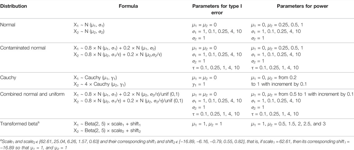
TABLE 1. Parameter setups for simulation studies.

To further evaluate the performance of the tests three possible scenarios arise for various combinations of σ₁ and σ₂ for normal, contaminated normal and contaminated with normal/uniform distributions as described later.

6.1.1 Normal

Scenario I: σ₁ = σ₂ represents the case of two normal distributions with equal variances.

Scenario II: σ₁ < σ₂ represents the case where variance of the second population is larger, and in evaluating power, it corresponds to the situation that the variance is larger for the second population with larger mean, that is, ${\mu }_2>{\mu }_1=0$

Scenario III: σ₁ > σ₂ represents the case where variance of the first population is larger, and in evaluating power, it corresponds to the situation that the variance is smaller for the second population with larger mean (μ₂ > μ₁ = 0).

6.1.2 Contaminated Normal

Scenario I: σ1 = σ₂ represents the case of two normal distributions with unequal variances (no contamination).

Scenario II: σ₁ < σ₂ represents the situation that the variance of the contaminated part of the distribution is larger, that is, contamination with the normal distribution with “outliers”.

Scenario III: σ₁ > σ₂ represents the situation that the variance of the contamination part of the distribution is smaller, that is, contamination with the normal distribution with “inliers”.

6.1.3 Combined Normal and Uniform

Scenario I: σ1 = σ₂ represents the case of two contaminated normal distributions, contaminated with normal/uniform (N/U) distribution, with equal variances.

Scenario II: σ₁ < σ₂ represents that the variance of contamination part of the distribution with N/U is larger, that is, contamination is done with “outliers” coming from N/U distribution.

Scenario III: σ₁ > σ₂ represents that the variance of contamination part of the distribution with N/U is smaller, that is, contamination is done with “inliers” coming from N/U distribution.

For cauchy and transformed beta, the distributions were simulated for the parameters given in Table 1.

6.2 Simulation Results

For ease of readability, we have reported the ratio of empirical estimate of type I error/expected level of significance, that is, $R=\widehat{\alpha }/\alpha$, for all tables and figures reporting type I error results so that for a well-controlled test the ratio should be close to 1.

Based on our extensive simulation studies, it is clear that for all the distributions under study, the empirical type I error rates were better controlled for both trimmed tests, $TRIM$ and $mTRIM,$ corresponding to 15% trimming proportions $(TRI{M}_{0.15},mTRI{M}_{0.15})$ compared to other trimming proportions (data not shown). In addition, from Table 2 (α = 0.001) and for α = 0.05 (data not shown), it is clearly seen that the type I error control for normal distribution for $TRI{M}_{0.15},$ $mMWW,$ $t,$ and $W$ are not maintained, and they get progressively worse with increasing stringent levels of α. Therefore, for all figures evaluating type I error and power properties, for the five distributions, we only included $mTRI{M}_{0.15}$ and its competitors $t_{BF},$ $T_{NB}^A,$ and $T_{NB}^P.$

TABLE 2

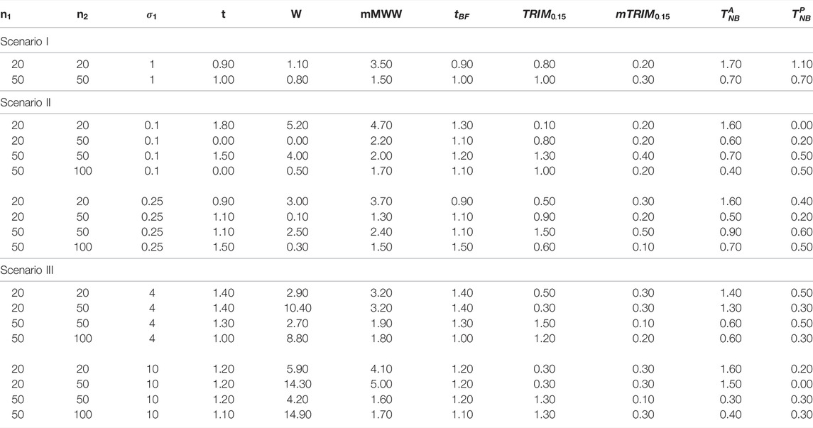
TABLE 2. omparison of the ratios for the eight methods under normal distribution ${\sigma }_2=1$ and $\alpha =0.001$.

Remark: In practice, the choice of trimming proportions would be critical. Our recommendation, supported by our simulation studies, is to use 15% trimming proportions because trimming less than that provides results that would be similar to the normal setting (type I error control often not maintained) and trimming more than that results in more conservative tests and loss of power. In general, higher proportion of trimming would be recommended for settings where the underlying distribution may be very heavy tailed. However, this would not be known a priori and would be a daunting task to check at each loci, particularly, in the context of high-throughput data, but a 15% trimming provides a balance between not trimming enough to trimming too much and generally provides reasonably good results for all underlying distributions (including asymmetric distribution) studied in our simulation studies.It may also be noted that we compared the null distributions at two levels of $\alpha =0.05$ and $\alpha =\mathrm{0.001.}$ We wanted to compare the performance of the test procedures at more stringent levels of α in the range of ${10}^{-4}$and ${10}^{-5},$ but this was not feasible for the permutation test as that would have required us to generate millions of samples to get reasonable estimate of type I error. However, we did estimate type I error control at stringent levels of α for $mTRI{M}_{0.15}$and found that the type I error control was strictly maintained for all the symmetric distributions and was somewhat conservative (data not shown).Extensive simulations studies corresponding to all combination of parameters mentioned in Table 1 were conducted, and the results were very similar, so a summary of the simulation results for each distribution, corresponding to a specific parameter combination, is discussed below. It is worth noting that the performance of the test procedures is relatively good for $\alpha =0.05,$ but it gets progressively worse as the type I error becomes more stringent. Thus, we discussed the results corresponding to $\alpha =0.001$ only. The results corresponding to α = 0.05 for the same parameter combinations are available from the authors on request. Also, the results corresponding to contaminated normal and combined normal and uniform were similar, so we chose to report the results corresponding to the combined normal and uniform distribution.

6.2.1 Normal Distribution

Null Distribution: As seen from Figure 1A, it is clear that, in general, the type I error control at $\alpha =0.001$ is well maintained with $mTRI{M}_{0.15}$ and $T_{NB}^P$being on the conservative side and $T_{NB}^A$being somewhat anti-conservative.

FIGURE 1

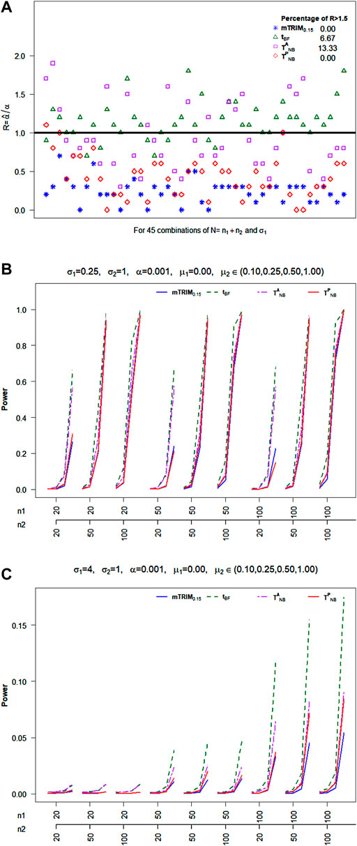
FIGURE 1. (A) Plot of ratio $\mathit{R}=\widehat{\mathit{\alpha }}/\mathit{\alpha }$ for normal distributions (α = 0.001). (B). Empirical power for normal distributions (Scenario II). (C). Empirical power for normal distributions (Scenario III).

Power Properties: For Scenario I, with ${\sigma }_1={\sigma }_2=1$ and $\alpha =0.001$(data not shown), it is seen that power for $t_{BF}$ and $T_{NB}^A$ are quite comparable with having slight advantage, as would be expected. $T_{NB}^P$ does slightly worse followed by $mTRI{M}_{0.15},$particularly when the sample size for one of the groups is smaller. For Scenario II, Figure 1B, taking ${\sigma }_1=0.1$ and ${\sigma }_2=1$ and $\alpha =0.001,$ once again the performance of $t_{BF}$ and $T_{NB}^A$ are quite comparable with $t_{BF}$doing slightly better. The performance of $T_{NB}^P$and $mTRI{M}_{0.15}$ are comparable with $mTRI{M}_{0.15}$ doing slightly better than $T_{NB}^P.$ For Scenario III, Figure 1C, taking ${\sigma }_1=4$ and ${\sigma }_2=1$ and $\alpha =0.001,$ the power for all tests is very low but $t_{BF}$ clearly dominates all other tests, and the performance of $mTRI{M}_{0.15}$ is the worst, but not by much.

6.2.2 Combined Normal and Uniform

Null Distribution: From Figure 2A, it is clear that $mTRI{M}_{0.15}$ has the best type I error control as the percentage of times R > 1.5 among all cases for the tests. $mTRI{M}_{0.15},t_{BF},T_{NB}^A$ and $T_{NB}^P$ are 0.89, 3.91, 20.89 and 6.40, respectively, when the true nominal level is $\alpha =\mathrm{0.001.}$Power Properties: For Scenario I, assuming ${\sigma }_1={\sigma }_2=1,$ $\tau =4$ and $\alpha =0.001,$ (data not shown), the performance of $mTRI{M}_{0.15}$ was comparable to $T_{NB}^P$ with slight advantage for $T_{NB}^P.$ The power estimates are higher for $T_{NB}^A$, but it fails to control type I error. The performance of $t_{BF}$ is the worst. For Scenario II, Figure 2B, ${\sigma }_1=0.1,$ ${\sigma }_2=1,$ $\tau =4$ and $\alpha =0.001,$ it is seen that, in general, $mTRI{M}_{0.15}$ has more power than $t_{BF}$ and$T_{NB}^P$ and is comparable to $T_{NB}^A$ but $T_{NB}^A$ does not control type I error well. For Scenario III, Figure 2C, ${\sigma }_1=4,$ ${\sigma }_2=1,$ $\tau =4,$ and $\alpha =0.001,$ the inliers problem, the trimmed test does worse than $T_{NB}^A$ and but the power, in general, is low. One should also keep in mind that the problem of “inliers” is less common in practice, and the trimmed test is designed to provide protection against “outliers” ; in the presence of outliers, the trimmed test performs well.

FIGURE 2

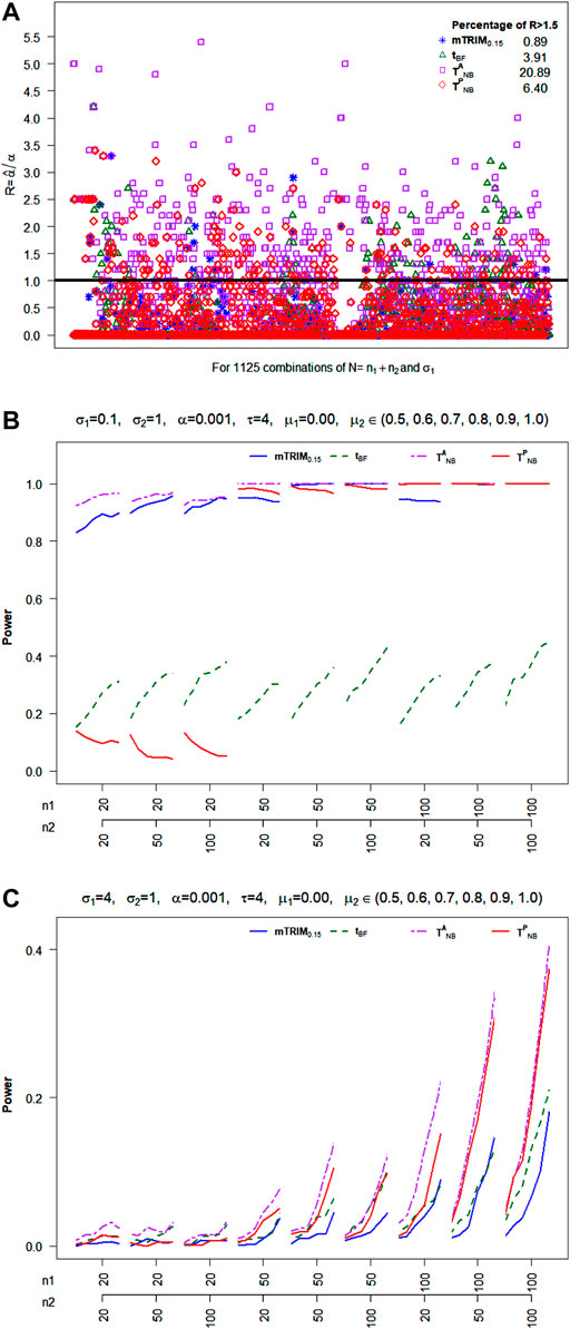
FIGURE 2. (A) Plot of ratio $\mathit{R}=\widehat{\mathit{\alpha }}/\mathit{\alpha }$ for the combined normal and uniform distribution for τ = 4 and α = 0.001. (B) Empirical power for the combined normal and uniform distribution (Scenario II). (C) Empirical power for the combined normal and uniform distribution (Scenario III).

6.2.3 Cauchy Distribution

For cauchy distribution, from Figure 3A, it is very clear that $mTRI{M}_{0.15},T_{NB}^P$ and $t_{BF}$ are conservative but $T_{NB}^A$ could be anti-conservative particularly for small sample sizes. From Figure 3B for power estimates, it is clear that the performance of $t_{BF}$ is the worst, and the performances of $mTRI{M}_{0.15}$ and $T_{NB}^P$ are comparable with having a slight advantage. $T_{NB}^A$ performs the best but one must keep in mind that often the type I error is not controlled, especially for smaller sample sizes.

FIGURE 3

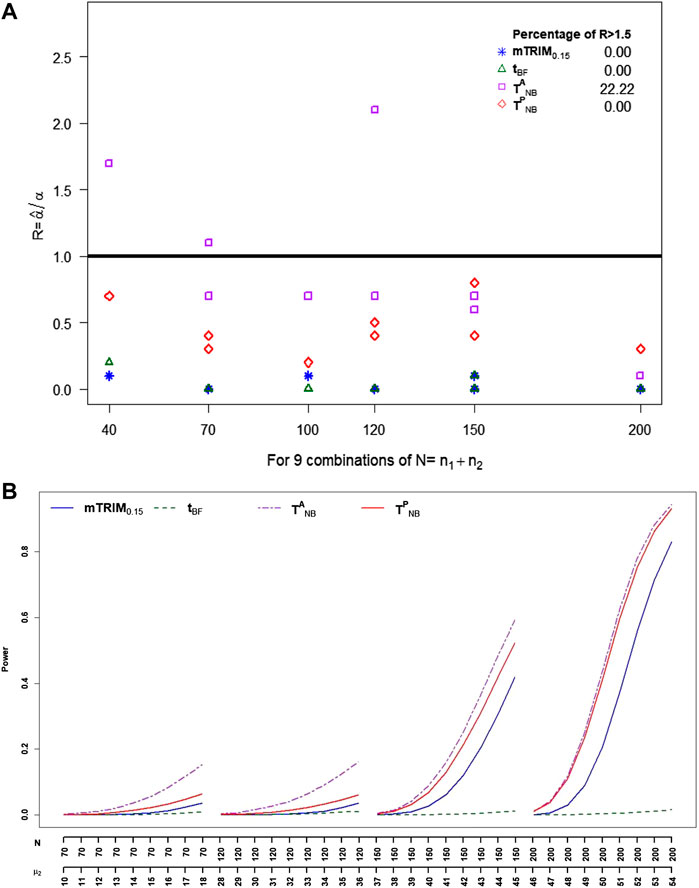
FIGURE 3. (A) Plot of ratio $\mathit{R}=\widehat{\mathit{\alpha }}/\mathit{\alpha }$ for the cauchy distributions α = 0.001. (B) Empirical power for cauchy distributions α = 0.001.

6.2.4 Skewed Transformed Beta

For skewed transformed beta distribution, from Figure 4A, it is very clear that none of the four tests can control type I error well. The percentage of times the type I errors exceeds 1.5 threshold for $mTRI{M}_{0.15},t_{BF},T_{NB}^A$ and $T_{NB}^P$ are 34.44, 50.00, 100.00, and 47.78, respectively. It may be noted that the percentage of times the type I errors exceeds the threshold of 2 for $mTRI{M}_{0.15},t_{BF},T_{NB}^A$ and $T_{NB}^P$ are 14.44, 31.11, 93.33, and 33.33, respectively However, from Figure 4B, it is very clear that the performance of $mTRI{M}_{0.15}$ and $t_{BF}$ are very comparable with $t_{BF}$ performing slightly better than $mTRI{M}_{0.15},$ which is consistent with the observation noted in Fagerland and Sandvik (2009). It may be noted that both $T_{NB}^A$ and $T_{NB}^P$ have higher power estimates, but the type I error is poorly controlled.

FIGURE 4

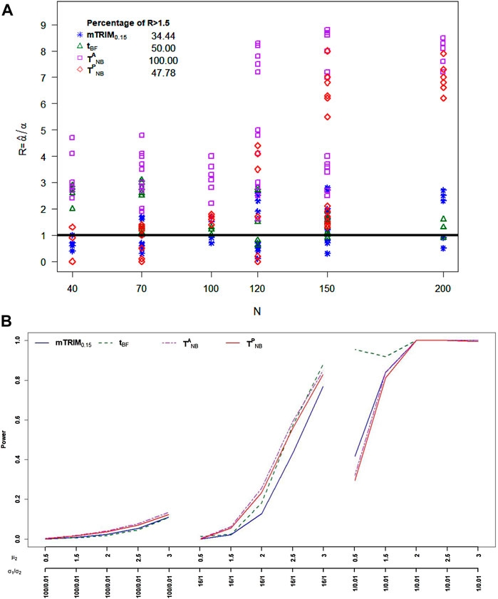
FIGURE 4. (A) Plot of ratio $\mathit{R}=\widehat{\mathit{\alpha }}/\mathit{\alpha }$ for transformed beta distribution α = 0.001. (B) Empirical power for transformed beta distributions for $N=n_1+n_2=100+50$.

7 Application to DNA Methylation Data

We downloaded the data from the NCBI Gene Expression Omnibus website and applied all the approaches discussed before to the example to evaluate their relative performances.

Figure 5 shows the histogram of p-values with the density estimates and the estimated FDR as a function of p-value cutoffs. The estimated non-null proportion are 0, 0.09, 0.28, 0.00005, and 0 corresponding to $mTRI{M}_{0.15},t_{BF},mMWW,T_{NB}^A$ and$T_{NB}^P$, respectively. From Figure 5, it is clear that the estimated $FDRs$ for $mMWW$ and $t_{BF}$ are not monotone functions of the p-value cutoff. Thus, conclusions drawn from such analysis would be misleading. The estimated $FDRs$ of $T_{NB}^A$ and $T_{NB}^P$ are 1 for all p-value cutoffs, but $T_{NB}^A$ and $T_{NB}^P$ output 24 and 17 p-values of exactly 0. For the DNA methylation data, if we set the significance level at α = 0.0001, then the number of SNPs identified to be significantly associated with the phenotype were 6, 7, 1, 24, and 17 corresponding to $mWMW,t_{BF},mTRI{M}_{0.15},T_{NB}^A$ and $T_{NB}^P,$ respectively. A histogram of the five most significant biomarkers for the two groups obtained based on $mTRI{M}_{0.15}$ is presented in Figure 6 to visually examine if the distributions of these markers can be perceived to be significantly different. For the marker cg15121304, it is clear that both distributions are skewed and probably no outliers, then based on our simulations results, we would expect $mTRI{M}_{0.15}$ and $t_{BF}$ to perform similarly as seen with p-values of 3 × 10⁻⁵ and 1.49 × 10⁻⁵, respectively. Furthermore, we expect $T_{NB}^A$ and $T_{NB}^P$ to produce highly significant p-values as they are not able to control type I error, which is confirmed with p-values of 0 for both tests. The distributions for the 4th and 5th marker (cg00491404 and cg16098170) are highly skewed and possibly have outliers, and in such situations, as seen from simulations, the p-values based on $T_{NB}^A$ and $T_{NB}^P$ tests are essentially 0 as we expected as they cannot control type I error rate (false positives), whereas those based on $mTRI{M}_{0.15}$ and $t_{BF}$ are not significant at level ${10}^{-4}$ suggesting that the results based on these two methods are similar and probably more conservative and believable. Of course, realizing that, in general, the $t_{BF}$ test would have significantly lower power than $mTRI{M}_{0.15},$ when the underlying assumptions are violated.

FIGURE 5

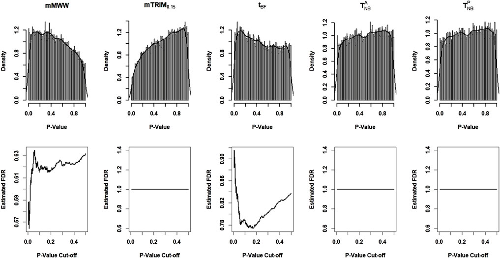
FIGURE 5. Results of the gene methylation array data corresponding to the five methods.

FIGURE 6

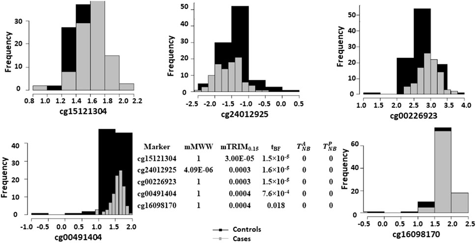
FIGURE 6. Histograms of logistic transformed methylation data for the five most significant markers based on the mTRIM_0.15 method and corresponding p-values for all the five methods.

8 Discussion

The proposed trimmed analog of the Behrens–Fisher statistic is robust in the sense that it can strictly maintain the type I error rate compared to the alternatives currently available in the literature and at the same time can provide significant gain in power when the underlying distributions may be in the neighborhood of normal with possibly unequal variances. However, it is possible that for some other underlying distributions and for some parameter combinations, other test procedures may outperform $mTRI{M}_{0.15}.$ However, based on the simulation studies, which include a broad range of symmetric heavy-tailed and skewed distributions, the example $mTRI{M}_{0.15}$ clearly outperforms its competitors in controlling the type I error rate, even at very stringent levels of $\alpha ,$ and has shown comparable power properties for a broad range of distributions. Thus, it provides for a viable alternative for comparing two distributions even when the assumption of normality or homoscedasticity may not hold. In the context of multiple hypotheses, it may not be feasible to test the assumption of normality and homoscedasticity simultaneously for all the hypotheses and then appropriately incorporate the findings in testing the hypothesis of interest using the most appropriate test. Thus, a procedure that can be implemented in broad settings that has reasonable robustness properties is needed and, we feel that the proposed trimmed statistic $mTRI{M}_{0.15}$ meets that need. Although, our simulation studies have focused on testing single hypothesis at stringent levels of $\alpha$, but since our test is on the conservative side (without much loss in power), it is not hard to visualize that by using the proposed test statistic one should be able to minimize false discoveries in the context of multiple hypotheses setting. It may be noted that the implementation of the trimmed test is straightforward and quick since we can use the well-known t-distribution with modified degrees of freedom. The computing time for $mTRI{M}_{0.15},$ $t_{BF},$ $T_{NB}^A,$and $T_{NB}^P$ (based on 10,000 permutations) were 0.001995087, 0.00199604, 0.009974957, and 9.892611 s, respectively, for one marker with 98 controls and 97 cases.

In a genome wide association study of a continuous outcome, often, we are interested in testing if the continuous outcomes corresponding to three genotypes are same or not. Furthermore, in a gene expression analysis of k samples, based on multiple dose levels, we could be interested in knowing if the gene expressions among k-sample are different or not. To address these issues, the commonly used parametric method will be ANOVA analysis if the data follow normal distribution; otherwise, the alternative of ANOVA will be the Kruskal and Wallis, 1952. However, similar to the two-sample comparison discussed in the study, it may be perceived that the two most popular methods may not be able to maintain type I error rate at a given significance level and may lose significant statistical power when the underlying distributions may not be normal and possibly heteroscedastic. We are currently in the process of investigating it and extending our approach to k-sample heteroscedastic case.

Often, the comparison in the two-sample case or k-sample case needs to be adjusted for covariates of interest that may be associated with the phenotype of interest. We are currently in the process of developing approaches that would provide robust comparisons after adjusting for the covariates.

Although the motivation and presentation of the method lies in identifying genetic features different between two groups, it is also readily applicable to any epidemiology studies of comparing continuous variables between two groups and any clinical trial of comparing continuous responses for two treatments. We have implemented the proposed method in R program (Supplementary Note S1). The method can be easily applied to compare the continuous variables between two groups from one to hundreds of thousands of tests.

Data Availability Statement

The methylation array data can be downloaded from publicly available data base at NCBI Gene Expression Omnibus (http://www.ncbi.nlm.nih.gov/geo) under accession no. GSE20067.

Author Contributions

All authors listed have made a substantial, direct, and intellectual contribution to the work and approved it for publication.

Funding

This research work of GK, SM, HZ, and DS was supported by the Grant CA21765 from the National Institutes of Health (NIH) and by the American Lebanese and Syrian Associated Charities (ALSAC). SR’s work was partially supported by the Wendell Cherry in Clinical Trial Research.

Conflict of Interest

Author LZ was employed by Eisai Inc.

The remaining authors declare that the research was conducted in the absence of any commercial or financial relationships that could be construed as a potential conflict of interest.

Publisher’s Note

All claims expressed in this article are solely those of the authors and do not necessarily represent those of their affiliated organizations, or those of the publisher, the editors, and the reviewers. Any product that may be evaluated in this article, or claim that may be made by its manufacturer, is not guaranteed or endorsed by the publisher.

Supplementary Material

The Supplementary Material for this article can be found online at: https://www.frontiersin.org/articles/10.3389/fsysb.2022.877601/full#supplementary-material.

References

Aspin, A. A. (1948). An Examination and Further Development of a Formula Arising in the Problem of Comparing Two Mean Values. Biometrika 35, 88–96. doi:10.1093/biomet/35.1-2.88

PubMed Abstract | CrossRef Full Text | Google Scholar

Benjamini, Y., and Yekutieli, D. (2007). The Control of False Discovery Rate in Multiple Testing under Dependence. Ann. Stat. 29, 1165–1188.

Google Scholar

Box, G. E. P. (1953). Non-Normality and Tests on Variances. Biometrika 40 (3/4), 318–335. doi:10.2307/2333350

CrossRef Full Text | Google Scholar

Brunner, E., and Munzel, U. (2000). The Nonparametric Behrens-Fisher Problem: Asymptotic Theory and a Small-Sample Approximation. Biom. J. 42, 17–25. doi:10.1002/(sici)1521-4036(200001)42:1<17::aid-bimj17>3.0.co;2-u

CrossRef Full Text | Google Scholar

Cao, H., Sun, W., and Kosorok, M. R. (2013). The Optimal Power Puzzle: Scrutiny of the Monotone Likelihood Ratio assumption in Multiple Testing. Biometrika 100 (2), 495–502. doi:10.1093/biomet/ast001

PubMed Abstract | CrossRef Full Text | Google Scholar

Chow, S. C., Shao, J., and Wang, H. (2008). Sample Size Calculations in Clinical Research. Chapman & Hall/CRC, Taylor and Francis Group.

Google Scholar

Cochran, W. G., and Cox, G. M. (1950). Experimental Designs. New York: John Wiley.

Google Scholar

Fagerland, M. W., and Sandvik, L. (2009). Performance of Five Two-Sample Location Tests for Skewed Distributions with Unequal Variances. Contemp. Clin. Trials 30, 490–496. doi:10.1016/j.cct.2009.06.007

PubMed Abstract | CrossRef Full Text | Google Scholar

Fligner, M. A., and Policello, G. E. (1981). Robust Rank Procedures for the Behrens-Fisher Problem. J. Am. Stat. Assoc. 76, 162–168. doi:10.1080/01621459.1981.10477623

CrossRef Full Text | Google Scholar

Hampel, F. R., Ronchetti, E. M., Rousseeuw, P. J., and Stahel, W. A. (1986). Robust Statistics: The Approach Based on Influence Functions. New York: John Wiley and Sons.

Google Scholar

Hochberg, Y., and Tamhane, A. (1987). Multiple Comparison Procedures. New York: Wiley.

Google Scholar

Huber, P. J. (1970). “Studentizing Robust Estimates,” in Nonparametric Techniques in Statistical Inference. Editor M. L. Puri (Cambridge, England: Cambridge University Press), 453–463.

Google Scholar

Janssen, A. (1997). Studentized Permutation Tests for non-i.i.D. Hypotheses and the Generalized Behrens-Fisher Problem. Stat. Probab. Lett. 36, 9–21. doi:10.1016/s0167-7152(97)00043-6

CrossRef Full Text | Google Scholar

Kang, G., Ye, K., Liu, N., Allison, D. B., and Gao, G. (2009). Weighted Multiple Hypothesis Testing Procedures. Stat. Appl. Genet. Mol. Biol. 8, 1–22. doi:10.2202/1544-6115.1437

CrossRef Full Text | Google Scholar

Kruskal, W. H., and Wallis, W. A. (1952). Use of Ranks in One-Criterion Variance Analysis. J. Am. Stat. Assoc. 47 (260), 583–621. doi:10.1080/01621459.1952.10483441

CrossRef Full Text | Google Scholar

Lee, A. F. S. (1995). Coefficients of lee-gurland Two-Sample Test on normal Means. Commun. Stat. - Theor. Methods 24 (7), 1743–1768. doi:10.1080/03610929508831583

CrossRef Full Text | Google Scholar

Lee, A. F. S., and Gurland, J. (1975). Size and Power of Tests for equality of Means of Two normal Populations with Unequal Variances. J. Am. Stat. Assoc. 70, 933–941. doi:10.1080/01621459.1975.10480326

CrossRef Full Text | Google Scholar

Mudholkar, A., Mudholkar, G. S., and Srivastava, D. K. (1991). A Construction and Appraisal of Pooled Trimmed-Tstatistics. Commun. Stat. - Theor. Methods 20, 1345–1359. doi:10.1080/03610929108830569

CrossRef Full Text | Google Scholar

Neubert, K., and Brunner, E. (2007). A Studentized Permutation Test for the Non-parametric Behrens-Fisher Problem. Comput. Stat. Data Anal. 51, 5192–5204. doi:10.1016/j.csda.2006.05.024

CrossRef Full Text | Google Scholar

Pagurova, V. I. (1968). On a Comparison of Means of Two normal Samples. Theor. Probab. Appl. 13, 527–534. doi:10.1137/1113069

CrossRef Full Text | Google Scholar

Pounds, S., and Rai, S. N. (2009). Assumption Adequacy Averaging as a Concept for Developing More Robust Methods for Differential Gene Expression Analysis. Comput. Stat. Data Anal. 53 (5), 1604–1612. doi:10.1016/j.csda.2008.05.010

PubMed Abstract | CrossRef Full Text | Google Scholar

Robins, J. M., van DER Vaart, A., and Ventura, V. (2000). Asymptotic Distribution ofPValues in Composite Null Models. J. Am. Stat. Assoc. 95, 1143–1156. doi:10.1080/01621459.2000.10474310

CrossRef Full Text | Google Scholar

Satterthwaite, F. E. (1946). An Approximate Distribution of Estimates of Variance Components. Biometrics Bull. 2, 110–114. doi:10.2307/3002019

CrossRef Full Text | Google Scholar

Shapiro, S. S., and Wilk, M. B. (1965). An Analysis of Variance Test for Normality (Complete Samples). Biometrika 52 (3–4), 591–611. doi:10.1093/biomet/52.3-4.591

CrossRef Full Text | Google Scholar

Srivastava, D. K., Mudholkar, G. S., and Mudholkar, A. (1992). Assessing the Significance of Difference between Two Quick Estimates of Location. J. Appl. Stat. 19 (3), 405–416. doi:10.1080/02664769200000036

CrossRef Full Text | Google Scholar

Storey, J. D. (2002). A Direct Approach to False Discovery Rates. J. R. Stat. Soc. Ser. B Stat. Methodol. 64, 479–498. doi:10.1111/1467-9868.00346

CrossRef Full Text | Google Scholar

Sun, W., and Tony Cai, T. (2009). Large-scale Multiple Testing under Dependence. J. R. Stat. Soc. Ser. B Stat. Methodol. 71, 393–424. doi:10.1111/j.1467-9868.2008.00694.x

CrossRef Full Text | Google Scholar

Teschendorff, A. E., Menon, U., Gentry-Maharaj, A., Ramus, S. J., Weisenberger, D. J., Shen, H., et al. (2010). Age-dependent DNA Methylation of Genes that Are Suppressed in Stem Cells Is a Hallmark of Cancer. Genome Res. 20 (4), 440–446. doi:10.1101/gr.103606.109

PubMed Abstract | CrossRef Full Text | Google Scholar

Tukey, J. W., and McLaughlin, D. H. (1963). Less Vulnerable Confidence and Significance Procedures for Location Based on a Single Sample: Trimming/Winsorization I. Sankhya, A 25, 331–352.

Google Scholar

Wald, A. (1955). Selected Papers in Statistics and Probability. New York: McGraw-Hill.

Google Scholar

Welch, B. L. (1949). Further Note on Mrs. Aspin’s Tables and on Certain Approximations to the Tabled Function. Biometrika 36, 293–296.

Google Scholar

Welch, B. L. (1947). The Generalization of “Student’s” Problem when Several Difference Population Variances Are Involved. Biometrika 34 (1-2), 28–35. doi:10.2307/2332510

PubMed Abstract | CrossRef Full Text | Google Scholar

Welch, B. L. (1937). The Significance of the Difference between Two Means when the Population Variances Are Unequal. Biometrika 29, 350–362.

Google Scholar

Yuen, K. K. (1974). The Two-Sample Trimmed T for Unequal Population Variances. Biometrika 61 (1), 165–170. doi:10.2307/2334299

CrossRef Full Text | Google Scholar