1
Department of Anesthesiology, Stony Brook University, Stony Brook, NY, USA
2
Medical Department, Brookhaven National Laboratory, Upton, NY, USA
3
Department of Neuroscience and Advanced Imaging Program, Mount Sinai School of Medicine, New York, NY, USA
4
Department of Neuroscience, McKnight Brain Institute, University of Florida, Gainesville, FL, USA
5
The National High Magnetic Field Laboratory, Tallahassee, FL, USA
In this study, a 3D digital atlas of the live mouse brain based on magnetic resonance microscopy (MRM) is presented. C57BL/6J adult mouse brains were imaged in vivo on a 9.4 Tesla MR instrument at an isotropic spatial resolution of 100 μm. With sufficient signal-to noise (SNR) and contrast-to-noise ratio (CNR), 20 brain regions were identified. Several atlases were constructed including 12 individual brain atlases, an average atlas, a probabilistic atlas and average geometrical deformation maps. We also investigated the feasibility of using lower spatial resolution images to improve time efficiency for future morphological phenotyping. All of the new in vivo data were compared to previous published in vitro C57BL/6J mouse brain atlases and the morphological differences were characterized. Our analyses revealed significant volumetric as well as unexpected geometrical differences between the in vivo and in vitro brain groups which in some instances were predictable (e.g. collapsed and smaller ventricles in vitro) but not in other instances. Based on these findings we conclude that although in vitro datasets, compared to in vivo images, offer higher spatial resolutions, superior SNR and CNR, leading to improved image segmentation, in vivo atlases are likely to be an overall better geometric match for in vivo studies, which are necessary for longitudinal examinations of the same animals and for functional brain activation studies. Thus the new in vivo mouse brain atlas dataset presented here is a valuable complement to the current mouse brain atlas collection and will be accessible to the neuroscience community on our public domain mouse brain atlas website.
Three-dimensional (3D) digital brain atlases have become indispensable tools for scientists in the neuroscience community. The 3D atlases are used to quantify accurately the volumes and shapes of brain structures, for statistical mapping of functional brain activation in a well-defined stereotaxic anatomical space, and for mapping of gene expression patterns (Brill, 2006
; Ng et al., 2007
; Schwaber et al., 1991
; Zaborszky and Vadasz, 2001
; http://www.brain-map.org/). The average human brain atlases that are based on hundreds of magnetic resonance imaging (MRI) scans of different normal individual brains and the probabilistic human brain atlases (Ahsan et al., 2007
; Ashburner and Friston, 2005
; Collins et al., 1995
; Evans et al., 1993
, 1994
; Hammers et al., 2003
; Holmes et al., 1998
; Mazziotta et al., 2001
) have facilitated discoveries of new specific morphometric signatures in several diseases including Alzheimer’s disease (Carmichael et al., 2005
; Chetelat and Baron, 2003
; Sowell et al., 2003
; Thompson et al., 2001
) as well as normal child brain development (Dager, 2007
; Lee et al., 2007
). These approaches may eventually become the gold standard for diagnosis as well as provide clues to alteration in neurocircuitry and gene expression patterns relevant for pathophysiology of a wide variety of diseases.
In parallel to human brain atlas neuroinformatics, morphometric studies of genetically engineered mouse models have also been undertaken to quantify and characterize brain anatomical ‘signatures’ under controlled genetic conditions. Until recently, morphometric data have most frequently been extracted by manually outlining regions of interest in the mouse brain MRI images and compared with corresponding data from wild-type controls. This approach has already lead to discoveries of gross abnormalities both in vivo and in vitro such as enlarged ventricles in vivo in a mouse model of transient cerebral ischemia (McDaniel et al., 2001
), hydrocephalus in SPAG6- and SPAG16L-deficient mice, a model of Knobloch syndrome (Zhang et al., 2007
), and hippocampal atrophy in a PDAPP mouse model of Alzheimer’s disease in vitro (Redwine et al., 2003
) which was not confirmed in vivo (Benveniste et al., 2007
). Volume changes in vitro in amyotrophic lateral sclerosis (ALS) mouse models of genetic (Özarslan et al., 2006
) or dietary origin (Petrik et al., 2007
; Wilson et al., 2004
) have also been demonstrated. Recently, Bock et al. (2006)
reported reduced cerebellar volume and other changes in the inferior colliculus and the olfactory bulbs in cdf mutant mice using both in vivo MRI and atlas-based semi-automated image analysis, demonstrating the utility of atlas-based neuroinformatics for mouse brain phenotyping.
Several 3D mouse brain atlases derived from formalin-fixed samples and in vitro magnetic resonance microscopy (MRM) technology with resolution below or near 100 μm in at least one image dimension (Benveniste and Blackband, 2002
) have recently become available (Badea et al., 2007
; Kovacevic et al., 2005
; Ma et al., 2005
; Mackenzie-Graham et al., 2004
). These newly published atlases are now increasingly being used as templates for semi- or fully- automated brain structure segmentation (Ali et al., 2005
; Badea et al., 2007
; Chen et al., 2005
) or for mapping of other rodent brain imaging modality data especially brain activation data acquired in vivo (Dorr et al., 2007
; Mirrione et al., 2007
; Zhang et al., 2007
). However, the atlas templates derived from in vitro specimens are not ideal for the mapping of in vivo data due to postmortem and/or the formalin fixation process which change brain shape and size. For example, the human average in vivo brain atlases (Montreal Neurological Institute brain or MNI brain) (Evans et al., 1993
) were designed in part to replace the postmortem single brain template of the Talairach and Tournoux atlas (Talairach and Tournoux, 1988
) for more accurate in vivo data interpretation. Thus, large discrepancies were found between the in vivo MNI average brain and the original Talairach coordinates (Brett et al., 2002
; Chau and McIntosh, 2005
; Lancaster et al., 2007
; Toga, 2002
; Uylings et al., 2005
; Van Essen, 2002
).
Similar to the human brain data it is reasonable to hypothesize that for analysis of in vivo mouse brain data, an in vivo atlas system would likely be more suitable. To our knowledge, there are no complete mouse brain atlas templates available that are derived from in vivo MRM images and there is also limited quantitative information in regards to morphological differences between in vivo and in vitro mouse brains. The general lack of in vivo mouse brain atlas templates is probably related to the challenges involved in acquiring in vivo MRM images with sufficiently high SNR and CNR to identify subtle and small anatomical structures (Benveniste and Blackband, 2002
). As a continuation of our previous mouse brain atlas work (Ma, et al., 2005
), we have constructed an adult male C57BL/6J mouse brain atlas database derived directly from in vivo T2-weighted 3D MRM images. To optimize the quality of the MRM images we designed new MR hardware and determined the most favorable parameters for contrast and SNR trade-offs. The new in vivo data are quantified and compared to our previous in vitro atlas data and demonstrate non-trivial and unexpected structural deformations caused by in vitro processing.
Animals and Preparation for Imaging
Inbred C57BL/6J male mice, 12–14-week old, weighing 25–30 g were used (Jackson Laboratory, Bar Harbor, ME). All protocols for live animal experiments were approved by the Institutional Animal Care and Use Committee. For MR microscopy (MRM) the mice were initially anesthetized with an intraperitoneal injection of a mixture of Nembutal (50 mg/kg), glycopyrrolate (0.01–0.02 mg/kg) and 0.9% saline. A gas mixture of oxygen and isoflurane (1–2%) was used for anesthesia maintenance. The electrocardiogram (ECG), respiratory rate and body temperature were monitored and recorded constantly with an MR-compatible small animal monitoring system (PC_SAM, model #1025, SA Instruments). The body temperature of the mouse was kept at 36.5°C and the respiratory rate was maintained around 50–65 bpm by adjusting the concentration of the isoflurane gas mixture.
MR Microscopy
All the in vivo mouse brain MRM images were acquired on a super-conducting 9.4T/210 mm horizontal bore magnet (Magnex) controlled by an ADVANCE console (Bruker) and equipped with an actively shielded 11.6 cm gradient set capable of providing 20 G/cm (Bruker, Billerica, MA). A birdcage radio-frequency (RF) coil (inner diameter 72 mm) was used as the transmission RF coil and a 30-mm-diameter surface RF coil as the receiver coil. We designed a new animal positioning system which provided more robust support to the animal cradle as well as better support of the RF birdcage coil against acoustic vibrations generated by the gradients and other sources. The new design also allowed us to place consistently the region of interest (i.e. the brain of the mouse) within the homogeneous center of the magnetic field (Figure 1
). The system comprises a long bore tube, which is supported at both ends via brackets attached directly to the exterior of the magnet cryostat (Figure 1
). Four foam ‘donut’ shaped gaskets within the bore help dampen acoustically induced vibrations of the bore tube (Figure 1
A). The second major part is the inner tube which holds the animal cradle and the surface coil mounted directly on fixtures built into the animal cradle (shown assembled in Figures 1
B,C). The mouse to be scanned is placed in the supine position with its head fixed on top of the center of the RF surface coil by the head fixture which also includes a mouth bar (for further details on the technical design see Smith et al., 2008
).
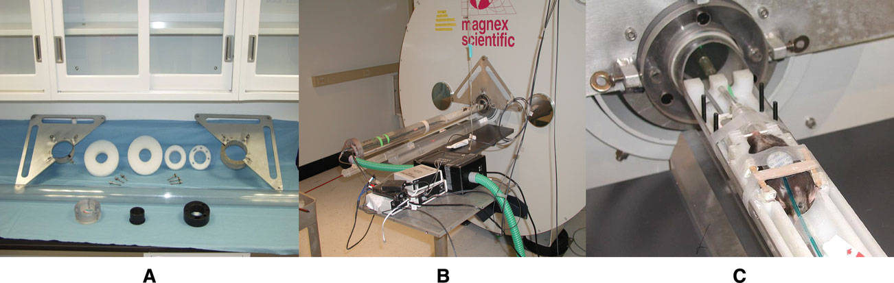
Figure 1. (A) Major parts of the positioning system. (B) Positioning system in place. (C) Mouse positioned supine in the stereotaxic cradle system which fits into the positioning tube that secures the RF volume coil in place.
MR Image Acquisition
T2-weighted MR data were generated with a 3D large flip angle spin echo sequence that shortens TR and the total scan time (Ali et al., 2005
; Bogdan and Joseph, 1990
; DiIorio et al., 1995
; Elster and Provost, 1993
; Ma et al., 1996
). In pilot experiments, optimal SNR and tissue contrast was achieved at a flip angle of 145° (number of excitations = 1; TE = 7.5 ms; TR = 400 ms). The mouse brains were imaged under two different spatial resolution schemes: 100 μm isotropic resolution (scan time ~2.8 hours) and 100 μm in-plane resolution with 200 μm slice thickness (scan time ~1.5 hours). The latter was implemented to determine the spatial resolution effects on the image contrast-to-noise, segmentation conditions and the accuracy of the resulted quantitative morphometry with the overall goal of reducing scan time if at all possible for future studies. The longest dimension of the mouse brain was set as the frequency encoding direction, with the remaining orthogonal directions sampled by phase encoding techniques. Image reconstruction was performed using Bruker Paravision software (version 4.0). A 3D fast Fourier transform was applied without any apodization, filtering or zero-filling. In all cases, 3D datasets were reconstructed into 16-bit grayscale images.
Creation of Individualized Atlases Using a Semi-Automatic Approach
In order to create individualized atlases, a first step is to define and segment the individual anatomical structures from the MRM images of the mouse brain. The segmentation procedure we used was essentially similar to that described previously (Ma et al., 2005
) with the exception that the first in vivo reference brain was segmented semi-automatically using our existing in vitro C57BL/6J mouse brain atlas (http://www.bnl.gov/ctn/mouse). The in vitro reference image was first registered with the in vivo image to be segmented (referred to as ‘target’ image) using linear and non-linear transformations [using both RVIEW (Studholme et al., 1996
) and AIR_5.2.5 software packages (Woods et al., 1998
)]. The same transformation parameters were subsequently applied to bring the atlas of the in vitro brain into registration with the target in vivo brain hereby producing a pilot segmentation of the target image. Due to registration errors and especially due to inherent morphological differences between in vitro and in vivo mouse brains (Figure 6
), the initial pilot segmentation did not match perfectly with the true structure boundaries in the in vivo image. Therefore the automatic segmentation result necessitated further smoothing and refinement which was done semi-automatically using a commercial 3D visualization and modeling software package (Amira 3.1, TGS, San Diego, CA).
The first segmented in vivo brain image was subsequently used as the new reference template to segment all other in vivo images since it registered better with the remaining in vivo group than the original in vitro reference brain. By repeating the above described processes a total of 12 in vivo mouse brain images were segmented. Each of the segmented in vivo data sets serves as an individualized atlas with 20 outlined brain structures which included: neocortex, hippocampus, amygdala, olfactory bulbs, basal forebrain and septum, caudate-putamen, globus pallidus, thalamus, hypothalamus, central gray, superior colliculi, inferior colliculi, the rest of the midbrain, cerebellum, the rest of the brainstem (i.e. pons and medulla), corpus callosum/external capsule, internal capsule, anterior commissure, fimbria, and ventricles. Quantitative structural information such as the averaged volumes and surface areas of each of the 20 structures were also extracted.
Creating the Average Atlas, the Probabilistic Atlas and Average Voxel Deformation Maps
A minimal deformation brain or an average brain is a simulated brain located in the geometric center of the population and represents the average shape and signal intensity of the group (Guimond et al., 2000
; Ma et al., 2005
). Therefore an average brain atlas is assumed to be a better representative of the whole group. The procedure of creating the average brain and atlas has been described in Ma et al. (2005)
. Initially, one of the individual brains and/or atlases was assumed to represent the group average. It was then iteratively updated based on the average transformation parameters of all the brains within the group and finally converged to the true geometric center of the group. As previously reported in Ma et al. (2005)
, we used the similarity index (SI) between two intermediate average atlases to monitor the convergence process. A similarity index close to 1 means little discrepancy between two intermediate average atlases and is an indication of convergence.
A probabilistic atlas contains structural spatial distribution information in the form of a probability within each voxel. The procedure for constructing the probabilistic atlas was the same as described in Ma et al. (2005)
. We used rigid-body transformation to align each individual in vivo brain image to the in vivo average brain template and then determined for each voxel the maximum probability of the structure spatial occupations. The probabi-listic atlas is a powerful tool for phenotyping and provides a priori probabilistic information for Bayesian based automatic segmentation algorithms (Ali et al., 2005
; Evans et al., 1994
; Mazziotta et al., 1995
, 2001
).
The average voxel deformation/displacement map was constructed by an initial linear and subsequent non-linear registration of all the individual brain atlases to the average brain atlas during which the non-linear voxel deformation was measured and recorded. By initially normalizing all individual brains through linear transformations, the deformation map represents a higher order average local geometrical difference within the group and provides direct visualization of these variations. In displacement/deformation maps, structural geometries within or between groups are revealed at the voxel level because the color coding at each voxel represents the average distance that each homologous voxel in the individual brains travels in order to register with the template brain. For example, the brighter the color, the bigger the distance a given voxel traveled to register with the template brain. For further details of the procedure of creating these atlases see Ma et al. (2005)
.
Statistics
Statistical evaluations of volume and surface area measurements were conducted on the extracted data from the 3D images acquired from the 12 mice in vivo. The volume and surface data of each of the 20 structures measured in vivo were compared with previous acquired in vitro data (Ma et al., 2005
) using an unpaired, two-tailed t-test. Intragroup data were analyzed using a paired t-test. A p-value < 0.05 was considered statistically significant.
Anesthesia and Animal Stability During Imaging
In spite of good fixation of the mouse head in the cradle using the mouth bar, the respiratory pattern often induced severe motion artifacts and hence compromised MRM image quality especially for longer scans. Figure 2
displays the time course of the spontaneous respiratory rate of seven individual C57BL/6J mice anesthetized with Nembutal and supplementary isoflurane inhalant gas during a 4-hour MRM scanning procedure. The figure demonstrates that the respiratory rate of the mice was stable during the first 2 hours (e.g. respiratory rate at 1 and 2 hours of scan time was 60.3 ± 9.6 bpm and 60.6 ± 9.6 bpm, respectively). However after 2 hours the respiratory rate trended towards being faster and more fluctuating in the later scan period (e.g. at 3.3 hours the average respiratory rate had increased to 69.8 ± 18.8 bpm, p < 0.05). The relatively non-fluctuating respiratory rate during the first 2 hours could be due to more stable physiological conditions (e.g. open airways, better pulmonary function and less compromise of respiratory muscles) in this initial time period.
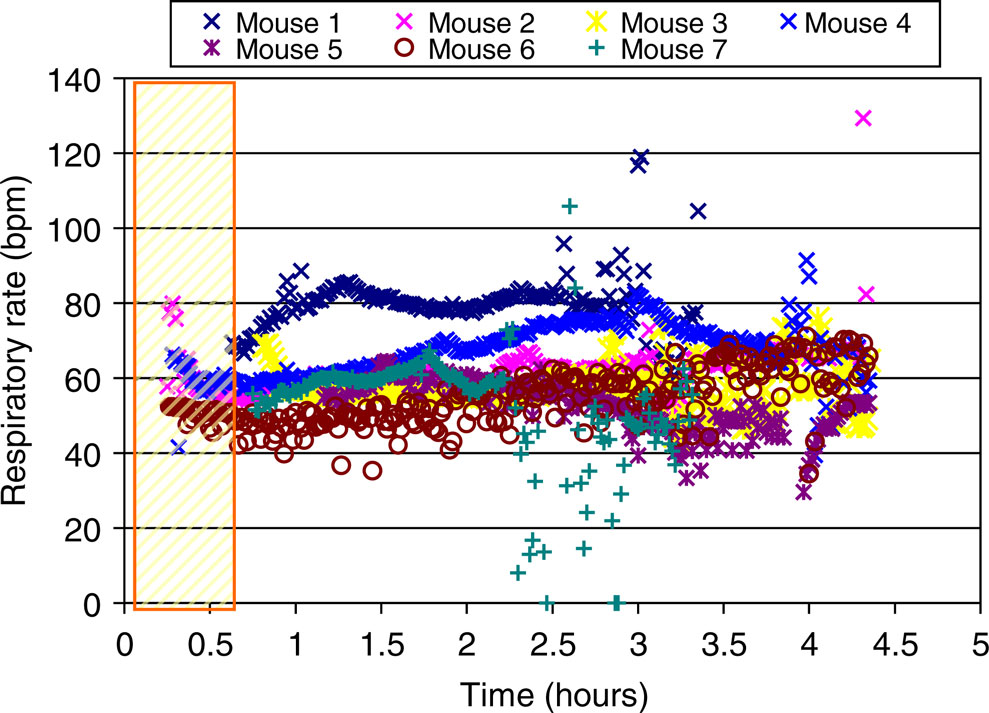
Figure 2. The time course of the respiratory rate of seven individual C57BL/6J mice during in vivo MRI scans (over 4 hours). The rectangle on the left represents the time period which was used for animal positioning, RF coil tuning and acquisitions of anatomical scout images to assure the correct positioning of the mouse brain in the center of the magnet.
Effect of Scan Time and Spatial Resolution on Segmentation
Considering the technical challenges and time demand involved in high resolution in vivo mouse brain imaging, we tested the effect of voxel size on MRM image segmentation. We acquired MRM images with a spatial resolution of 100 × 100 × 200 μm3 requiring 1.5 hour scan time and 100 × 100 × 100 μm3 requiring about 2.8 hours of scan time. Approximately 30% of the 3-hour higher resolution scans were discarded due to motion artifacts and/or animal death which we attribute largely to respiratory failure. In contrast, 95% of the lower resolution scans were successful. Figure 3
shows the clear difference in CNR between the low- and high-resolution scans. For example, the substructures in hippocampus such as the CA1, the hippocampal sulcus and the dentate gyrus were poorly defined on the low-resolution scans. Figure 4
shows the percentage difference between the 20 brain structure’s volumes and surface areas derived from the lower resolution (n = 12) and the high resolution groups (n = 12). As can be observed, for smaller structures such as the fimbria, the anterior commissure or the globus pallidus, the percentage difference in volume and surface area tended to be slightly larger (although not statistically significantly). For example, the volume of fimbria was 22.7% smaller measured from lower resolution scans than from higher resolution scans. In order to maximally reveal subtle structure details, we used the higher resolution scans to create the presented in vivo atlases. But for the majority of brain structures, the lower resolution scans are clearly adequate in volume and surface area measurements (Figure 4
). This information is important when designing future in vivo phenotyping experiments where limiting scan time is desirable in physically fragile transgenic mouse models of human diseases.
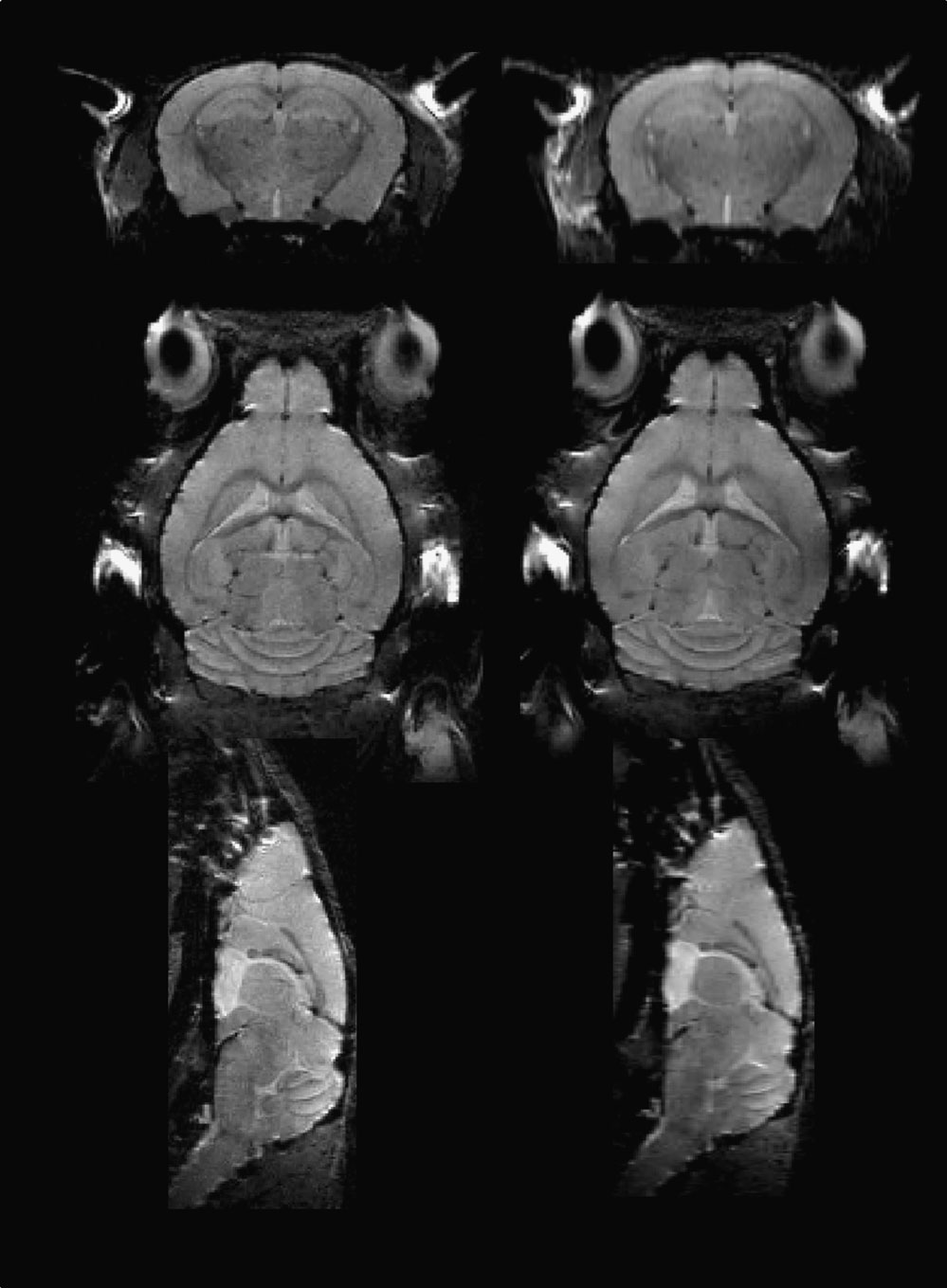
Figure 3. Left column: 100 μm isotropic-resolution scan; Right column: 100 × 100 × 200 μm3 resolution scan.
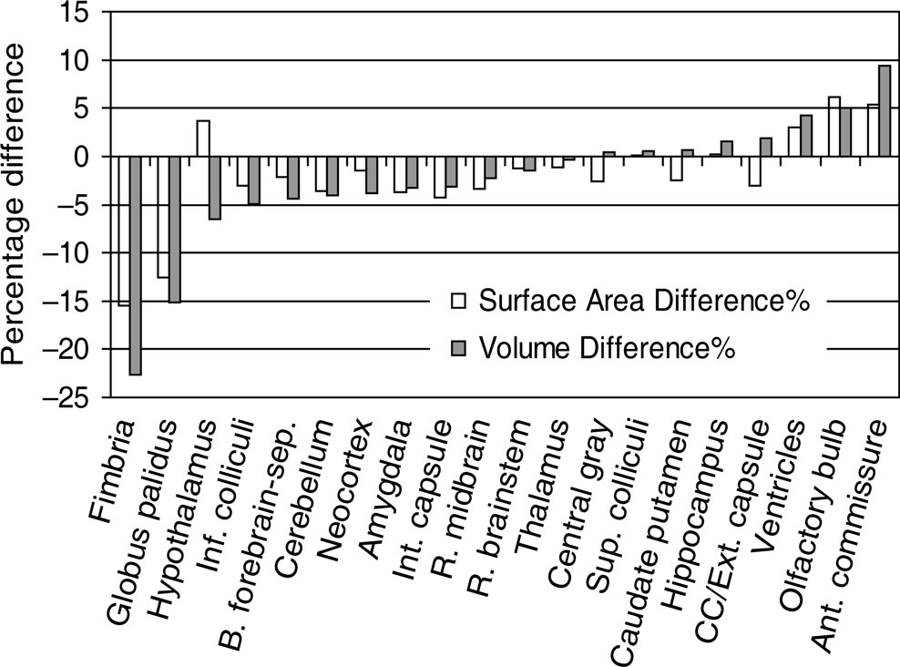
Figure 4. The percentage difference in structural volume and surface area measured from two different resolutions. The percentage difference was calculated as the measurement from the lower resolution scans (100 × 100 × 200 μm3, n = 12) subtracted that from the higher resolution scans (100 × 100 × 100 μm3, n = 12) and then divided by the former measurement. None of the structural differences were statistically significant (unpaired t-test). The abbreviations used are: Inf. colliculi = Inferior colliculi; B. forebrain-sep = Basal forebrain and septum; Int. capsule = internal capsule; R. midbrain = the rest of midbrain; R. brainstem = the rest of brainstem (i.e. pons and medulla); Sup. Colliculi = Superior colliculi; CC/Ext capsule = corpus callosum/external capsule; Ant. Commissure = Anterior commissure.
The In vivo C57BL/6J Atlas and Database
In the following sections, for optimal data analysis and description, all visual and quantitative assessments of the new in vivo C57BL/6J mouse data were compared with previously published in vitro C57BL/6J mouse data (Ma et al., 2005
).
The individual atlases. Figure 5
A shows the representative axial, coronal and sagittal slices from an in vivo MRM C57BL/6J mouse brain dataset. Figures 5
B–D display the corresponding reconstructed atlas surface in 3D. We were able to identify and segment 20 different anatomical regions from the in vivo images. However, certain parts including the boundaries of the posterior hypothalamic area, the globus pallidus, the caudate-putamen and the fine extensions of the white matter fibre tracts were challenging to define and we had to rely on parallel visual comparisons with existing 2D histologic atlases (Franklin and Paxinos, 1997
; Hof et al., 2000
) for complete segmentation of these regions.
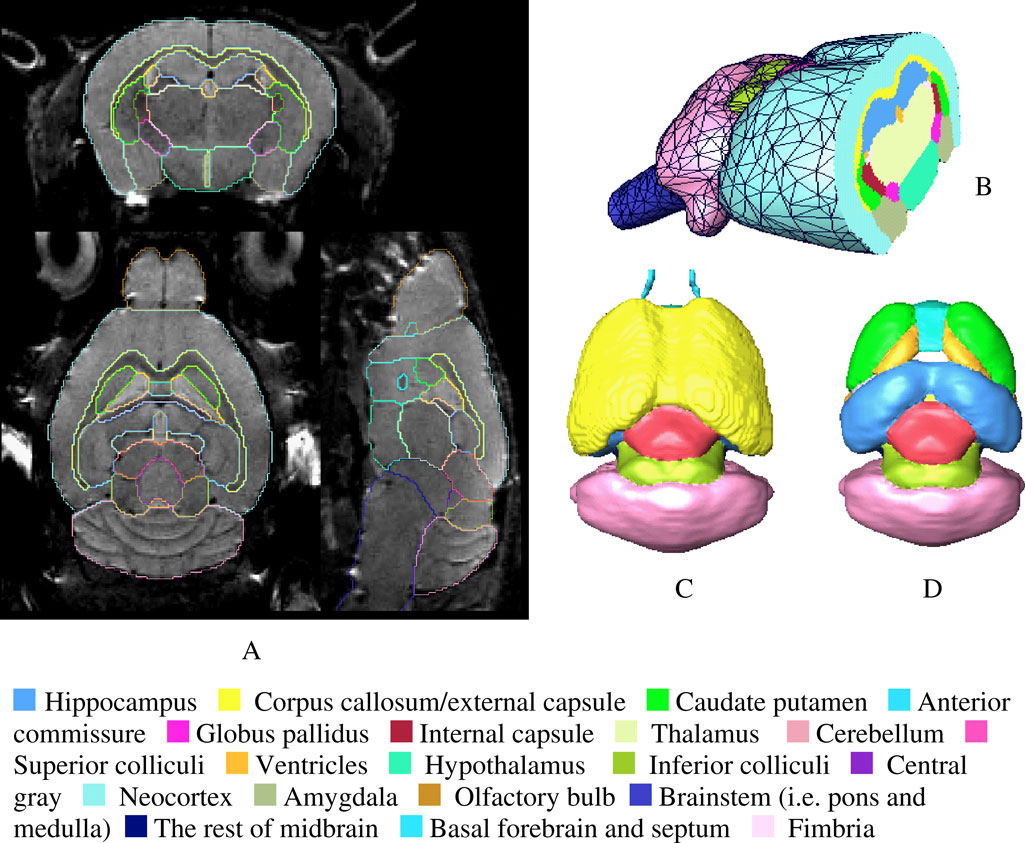
Figure 5. (A) The coronal, axial and sagittal slices of a 3D in vivo MRI mouse brain image with its structural segmentation superimposed as colored lines. (B) 3D surface reconstructed atlas with one cross section. (C) The brain interior with neocortex, olfactory bulb and brain stem hided from the view. (D) Further 3D details with the exterior capsule and the anterior commissure hidden from the view.
In Figure 6
, we have compared representative sections from the new in vivo mouse brain data and the previous in vitro data (Ma et al., 2005
) side by side. Apart from the obvious differences in overall CNR and SNR, the most significant visual difference between the two types of images was the appearance and size of the ventricles. In vitro, the ventricles had shrunk to such a degree that most parts of the third and fourth ventricles were not identifiable (and consequently not included in Ma et al., 2005
). Other structural differences between the in vivo and the in vitro brains were also indirectly revealed during the semi-automatic segmentation process. For example, a combination of an initial linear and a subsequent 169-parameter non-linear warping (in AIR_5.2.5) had to be applied to achieve an acceptable ‘fit’ when registering the in vitro templates with the individual in vitro brain images. In comparison, when registering two in vivo specimens, a rigid body registration based on mutual information (in RVIEW) alone would render an acceptable pilot segmentation.
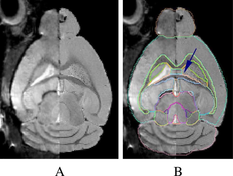
Figure 6. (A) The side-by-side difference of an in vivo (left half of the image) and an in vitro brain (right half of the image). (B) The in vivo atlas superimposed on (A). The ventricles are barely visible in the in vivo image (left half of the image) (as pointed out by the arrow and outlined by the in vivo atlas).
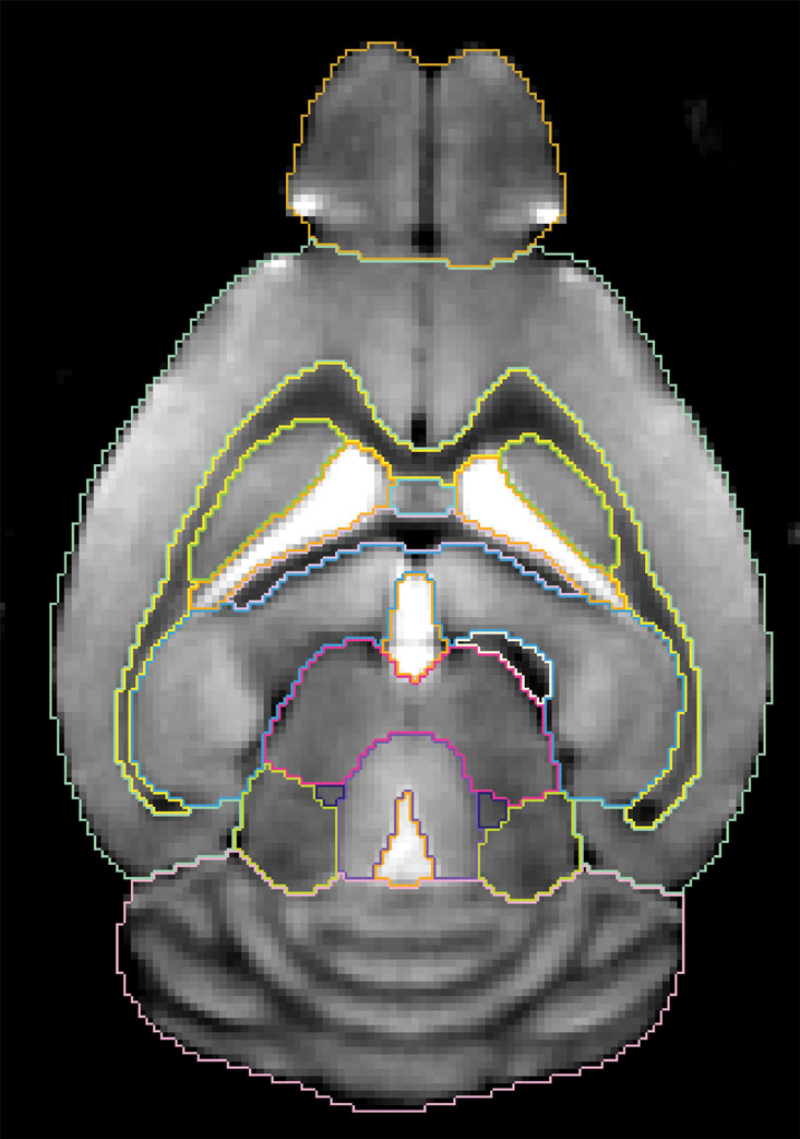
The average mouse brain/atlas and derived voxel deformation maps. Figure 7
shows an axial slice from the constructed average in vivo MRM brain with its corresponding atlas superimposed. As expected the average brain has better SNR than any of the individual in vivo brain MRM images (compare with Figures 3
,5 and 6
). During the iterative construction process of the average in vivo atlas, the convergence index reached 0.99 to 1 for all structures at the third iteration whereas for the corresponding in vitro average brain atlas (Ma et al., 2005
), an overall convergence index of 0.98 to 1.0 required five iterations. The fact that less iteration were needed for convergence among the in vivo brains is suggestive of less general geometric variability of the in vivo group compared to the in vitro group.
To further quantify and visualize the geometrical differences between the in vivo and in vitro brains at the voxel level, we created a series of voxel displacement/deformation maps within and between the two groups. Figure 8
shows the resulted average voxel deformation maps from (1) mapping each of the ten in vitro brains to their average in vitro atlas template (Figures 8
A,D); (2) mapping the 12 in vivo mouse brains to their average in vivo brain atlas (Figures 8
B,E,G) and (3) mapping each of the 10 in vitro brain to the in vivo average brain (Figures 8
C,F). We wish to point out that the deformation/displacement values were only measured during the 169 parameter non-linear warping in AIR_5.2.5 (i.e. the voxel displacements occurred during rigid-body or affine transformations in the initial registration process were not included) in order to exclude the linear variations such as scale and orientations of individual brain images. Also, the distance maps bear unavoidable registration errors especially for the smaller structures which are harder to be correctly registered, such as external/internal capsules, ventricles and fimbria. Therefore care has to be taken when interpreting the deformation maps at these locations.
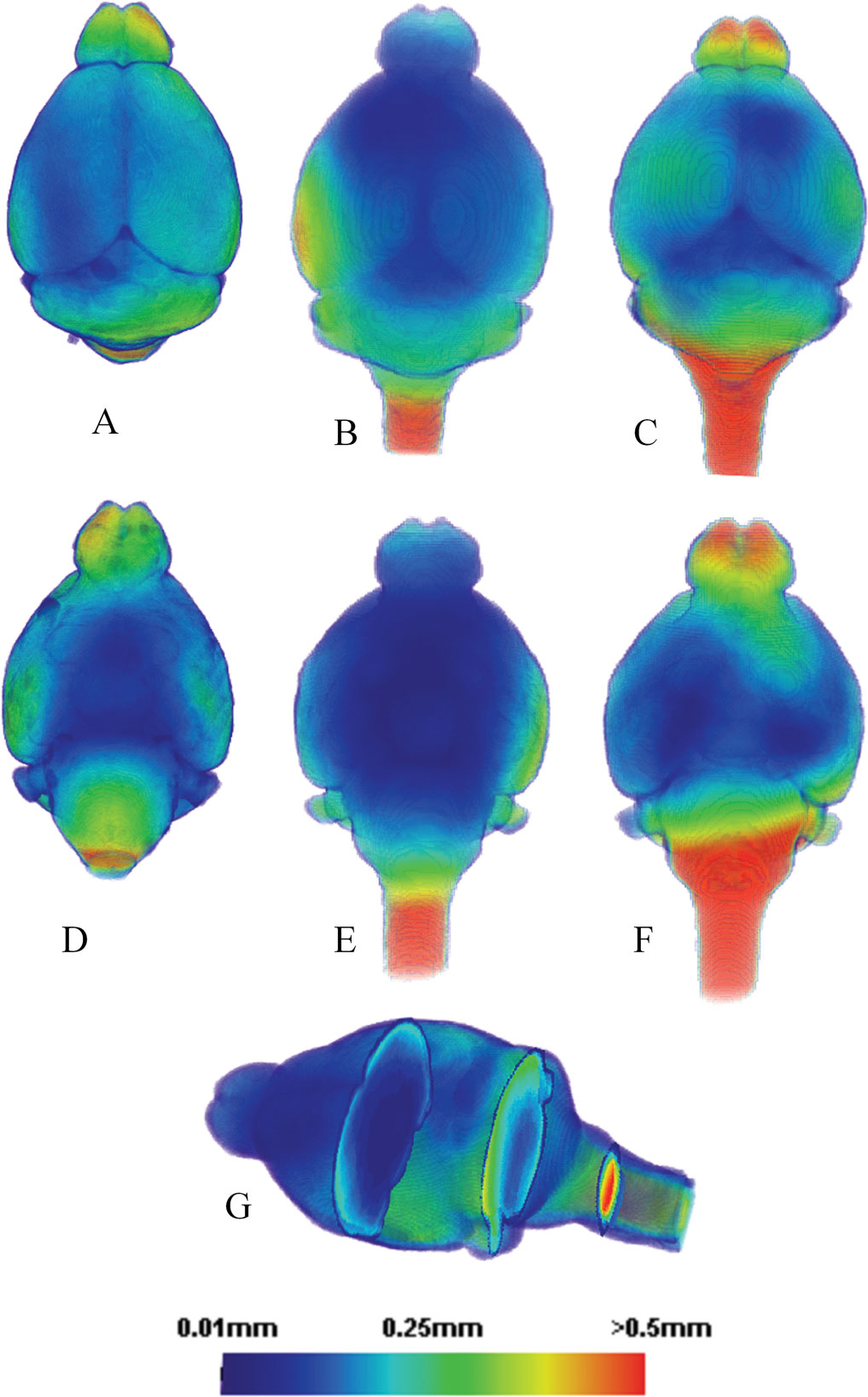
Figure 8. The average local deformation maps of: (A) 10 in vitro individual mouse brains mapped to the average in vitro brain. (B) 12 in vivo individual mouse brains mapped to the average in vivo brain. (C) 10 in vitro individual mouse brains mapped to the average in vivo brain. (D), (E) and (F): The ventral views of (A), (B) and (C), respectively. (G) A cross sectional view of (B) and (E). Note: the images are not strictly proportional. The color represents the average distance a given voxel underwent following registration of each of the individual brains to the average brain template.
When visually comparing the geometrical deformation map of the in vitro group (Figures 8
A,D) with that of the in vivo group (Figures 8
B,E), it is clear that for both conditions (formalin-perfusion/in vitro versus in vivo), the cerebellum, neocortex, olfactory bulbs and the brainstem contained surfaces with the largest displacements whereas structures located more centrally displayed the least. Furthermore, the in vitro group displayed more areas with quantitatively higher displacement values than the in vivo group, especially at the level of the cerebellum and olfactory bulbs. For both conditions, displacements greater than 0.5 mm mostly occurred at the level of the brain stem (Figure 8
). In vitro, the brain stems were curved much more ventrally (Figures 8
A,D); in vivo, the curvature of the brain stems also varied greatly probably due to different positioning of the animal’s cervical spine which would affect the shape of brain stem. Interestingly, the in vivo displacement map revealed a slight left-wards neocortical asymmetry (Figure 8
B).
Figures 8
C,F show (on a voxel by voxel level) the local deformations the in vitro brains had to undergo when ‘conforming’ themselves to the average in vivo brain and thus directly display the geometric alterations between the two groups in 3D. Figure 8
B can therefore be directly compared to 8C because both groups were mapped to the same in vivo average brain template. It is evident from the color coding that the areas in vitro associated with largest deformations when matching to the in vivo average brain were located frontally and caudally. We measured the statistical significance of the different local deformation characteristics of both groups (Figures 8
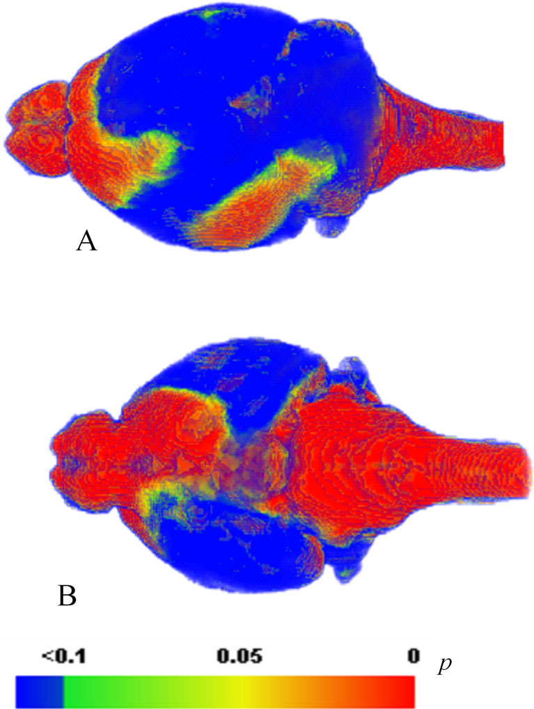
B,C) by using a voxel-wise unpaired student t test. Figure 9
shows the result of the t-test and confirms that the brain stem, olfactory bulb, and cerebellum display significantly larger deformations in vitro compared to in vivo. Furthermore, structures located ventrally show larger in vitro ~ in vivo differences than structures located dorsally.
Volume and surface areas of the 20 brain structures. Table 1
lists the average volume and surface areas of each of the 20 segmented regions of the new in vivo brain data as well as quantitative comparisons with the previous collected in vitro data (Ma et al., 2005
). Please note that in Table 1
, the structure names marked with a ‘*’ signifies that the percentage changes were measured from the in vitro average atlas instead of from the individual in vitro brains in order to reduce the effects of the brain stem (which is often damaged in vitro) and account for the slightly different olfactory bulb partitioning during the construction of the in vivo atlases in which the piriform cortex was included as part of the olfactory bulb (the in vitro average atlas has been updated to be consistent with the partitioning of the in vivo atlases). We also computed the total brain volume and surface area with or without including the brain stem and both measurements show significant total brain volume reduction in vitro (6.5% reduction measured without brain stem or 10.1% reduction with brain stem, p < 0.01).
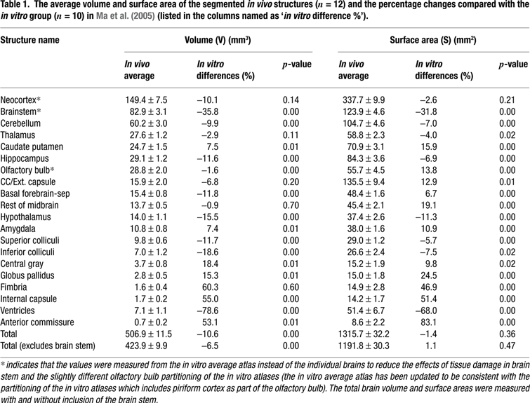
Table 1
shows that the standard deviations and thus intragroup variability of the in vivo brains are very minor with individual regional volume standard deviation ranging from 0.2 mm3 (internal capsule and anterior commissure) to 7.5 mm3 (neocortex). Importantly Table 1
also demonstrates that among all of the in vitro structures, the ventricles exhibited the most significant shrinkage (78.6% decrease in volume and 68% decrease in surface area with p < 0.01) compared to the in vivo data, which is consistent with previous visual observation. Additionally, the following structures showed significant volume and/or surface area reduction in vitro versus in vivo: the brain stem, the cerebellum, the olfactory bulbs, the hypothalamus, the superior colliculi, the inferior colliculi, the hippocampus, the basal forebrain and the septum. Interestingly, as further noted in Table 1
, the following structures show expansion in vitro including the caudate putamen, the amygdala, the central gray, the globus pallidus, the internal capsule and the anterior commissure. It is at present unknown why some structures are more affected and shrink while others are unaffected or expand. For smaller structures such as the internal capsule, the anterior commissure, the fimbria and the external capsule, the results may be unreliable due to segmentation errors secondary to inferior SNR, spatial resolution and volume averaging in vivo compared to in vitro. Alternatively, the various brain regions may be more or less affected by the ventricular space collapse and undergo different shear stresses in vitro, resulting in either expansion or shrinkage. This might for example explain why the caudate putamen expands because it is located adjacent to the ventricles. However we have not attempted to model or test this theory. The regional differences in myelin content might also play a role but we have no systematic measure for how this relate to the volumetric changes at this time.
The probabilistic atlas. Figure 10
shows the in vivo probabilistic atlas in 3D and in cross-section. The bright red color corresponds to the probability of 1 indicating that all the 12 brains have the same structure and/or shape at this location. The lower probabilities are represented by green and blue colors indicating higher group variability. As can be observed, the variability was generally very small inside each structure. Higher variability typically occurred at structure boundaries such as towards the cortical surface, the surface of the cerebellum, brain stem and smaller structure boundaries such as the external capsule, the internal capsule and the anterior commissure. In addition, hard-to-define boundaries such as those between the hypothalamus and the thalamus or between the superior and inferior colliculi were also prone to low probability values which could indicate errors caused by possible segmentation inconsistencies at these locations. Furthermore, it is well-known that registration errors affect smaller structures more than larger structures which could also contribute to the lower probabilities observed at the boundaries of small and narrow structures such as white matter tracts. The probability atlas also shows that the brain stem displays a lower interior probability than any other structure primarily due to the inconsistent positioning of the animal’s cervical spine during MRM scans.

Figure 10. (A) The 3D in vivo probabilistic atlas with three cross sections at different locations. The colors in the cross section show at each voxel the maximum probability of the common structure occupied by the normal C57BL/6J mouse brains (n = 12) after rigid-body alignment. The bright red color corresponds to high probability; blue color corresponds to low probability. (B) One cross section of the in vivo probabilistic atlas is displayed together with the average brain surface (The colors on the brain surface represent different structures).
The major results of this study are (1) the presentation of an in vivo C57BL/6J brain atlas derived from MRM images with 20 different anatomical structures identified; (2) quantitative meta data (e.g. volumes and surface areas of the 20 structures) demonstrating minimal intragroup variability among the 12 in vivo genetically identical C57BL/6J mouse brains; (3) an average in vivo MRM atlas template of the C57BL/6J mouse brain (n = 12); (4) a corresponding in vivo C57BL/6J probabilistic atlas; (5) a local group deformation map based on the 12 in vivo C57BL/6J mice brains demonstrating the intragroup voxel-wise geometrical variations and finally (6) quantitative data defining differences between in vitro and in vivo C57BL/6J mouse brain morphometry.
In vivo MRM Mouse Brain Images
Choice of T2-weighted pulse sequence. In this study our goal was to create an in vivo C57BL/6J mouse brain atlas using MRM technology. We therefore strived to create the best possible MRM images from the point of view of SNR and brain anatomical CNR, while at the same time considering the necessary tradeoffs to be taken to reduce the total scan time. We chose to use a T2-weighted 3D MRM sequence with a large flip angle which would reduce TR and therefore scan time while at the same time preserving its T2-weighting (Ali et al., 2005
). T2-weighted MR contrast is advantageous for imaging rodent brain anatomy in comparison with T1 weighted sequences (Benveniste et al., 2000
). The shortened TR allowed us to achieve a spatial resolution of 100 μm in less than 3 hours. Several other time-efficient T2-weighed sequences [e.g. T2-weighted rapid acquisition with relaxation enhancement (RARE) pulse sequence] are available which also provide high tissue CNR, but our initial pilot tests showed the images with RARE factors greater than 8 were more subject to motion artifacts causing lower success rates, i.e. inferior SNR and CNR (data not shown). Reducing the RARE factor will typically increase scan time (from increased signal averaging) in order to achieve similar image quality. For example using a 3D RARE sequence with the following parameters: TR of 1.2 s, RARE factor of 4, isotropic resolution of 100 μm and two signal averages would require about 4.2 hours of scan time, assuming that no anti aliasing factors would be required in the two phase encoding directions.
Physiological and non-physiological motion. MRM images acquired in vivo are affected by the physiological motion from the beating heart, the diaphragm and involuntary reflexes from the airways. The image artifacts from physiological motion can be minimized to some extent by immobilizing the head of the animal and/or using pulse sequences that are acquiring data synchronously with the ventilation and cardiac activity. We did immobilize the head of the animal using our custom build animal cradle but did not implement scan-synchronous ventilation as the total scan time would have increased dramatically. For example, with a spontaneous respiratory frequency of 60 bpm the effective TR would have increased from 0.4 s to 1 s and consequently increased scan time from 2.8 hours to 7 hours).
The animals had to be anesthetized, immobile and physiologically stable for the scan duration to minimize motion artifacts. Our anesthetic regimen included the hypnotic pentobarbital (Nembutal) and supplemental isoflurane inhalant gas administered to the spontaneous breathing mouse as needed to maintain the depth of anesthetic state. The time course of the breathing pattern over the 3–4 hours experimental period revealed a stable breathing pattern during the first 2 hours and a more fluctuating one in the later period of the scanning (Figure 2
). The more erratic breathing pattern after 2 hours could be contributed to by different anesthesia effects and/or general compromise of the respiratory function. In rodents the anesthesia duration with 50 mg/kg Nembutal administered i.p. is about 30–60 minutes (Laber-Laird et al., 1996
). Therefore, in order to maintain the respiratory frequency around 60 bpm, isoflurane was typically added on in escalating concentrations after 30–60 minutes when Nembutal was wearing off. However, both Nembutal and isoflurane interfere with the animal’s respiratory effort by decreasing the tidal volume as well as the respiratory frequency. Therefore the more irregular breathing pattern was more likely due to general respiratory compromise secondary to prolonged spontaneous breathing under anesthesia in the supine position. For example, during normal spontaneous ventilation, the rib cage and the diaphragm contribute more to the thoracic expansion. With induction of anesthesia, the functional residual capacity decreases as the diaphragm flattens which contributes to the formation of atelectasis (Miller, 2005
). Furthermore, most anesthetics also affect pulmonary and laryngeal stretch receptors leading to tachypnea and low tidal volumes, which can inevitably lead to an unstable respiratory pattern (Miller, 2005
). We are currently working on refining our anesthesia technique to further decrease this problem for future studies.
Non-physiological motion originating from the MR instrument itself in the form of vibrations (acoustical) from the activity of strong gradients can also interfere with image quality. We designed and implemented a new animal cradle/holder and positioning system to circumvent this problem. The new positioning system stabilized and maintained the position of the anesthetized animal and at the same time also secured the two RF coils’ positions in relation to the area of interest (e.g. the mouse brain). In contrast to most commercial MR instruments where the animal positioning devices are designed as cantilevers attached to a table in front of the magnet, our system (i.e. the outer tube of the positioning system) is supported at both ends and fixed to the outside of magnet. It is thus ‘free-floating’ inside the magnet bore and isolated from the gradient inserts which helps dampen the vibration noise generated by the gradients during imaging (Smith et al., 2008
).
Mouse brain anatomy revealed on the T2-weighted MRM images. The 3D T2-weighted MRM in vivo images which we acquired were of sufficient quality to allow the identification of 20 different mouse brain structures, but there were several structures and anatomical borders which were hard to define on the in vivo images. In our previous in vitro mouse brain atlas MRM study, we were also able to identify 20 brain regions on the T2*-weighted high resolution images (47 μm isotropic) which were acquired on a 17.6T MR instrument and these images clearly had superior CNR compared to the in vivo images acquired here (cf. Figure 6
). Previously, the anatomical segmentation of the in vitro images was also associated with difficulties especially when defining certain areas such as the boundaries of the posterior hypothalamic area, the boundary of the thalamus and pretectum as well as the fine extension of white matter tracts (Ma et al., 2005
). Some of the same areas which could not be accurately defined on the in vitro images were also difficult to define in vivo, for example the borders of the posterior hypothalamic area and white matter tracts. On the other hand, additional areas were prone to segmentation inaccuracies in vivo including the globus pallidus and the caudate-putamen which were more clearly visualized in vitro (Ma et al., 2005
), demonstrating the different CNR characteristics of in vitro and in vivo studies.
In vivo Compared to In vitro
Our idea to create an in vivo C57BL/6J mouse brain atlas database including an average brain atlas originated from the human brain neuroinfomatics literature demonstrating that an average in vivo human brain atlas (e.g. the MNI brain atlas) derived from hundreds of different MRI brain scans is a better anatomical representation of the general population and from a statistical point of view therefore is more accurate for interpreting in vivo data (Chau and McIntosh, 2005
; Lancaster et al., 2007
). In contrast to the MNI brain atlas derived from MRIs of many individual brains with different genotypes and environmental exposures, the 12 C57BL/6J mice used in this study were genetically identical and had been exposed to the same environment during their lifespan. It is therefore not surprising that our in vivo data demonstrated minimal group variability. Similar to the human literature we documented morphometric differences between the in vivo brains and the formalin-fixed in vitro brains. First, the statistical test on the voxel-wise displacement maps derived from in vitro and in vivo datasets demonstrated significantly larger deformations in vitro in the areas of the brain stem, the olfactory bulbs, cerebellum and frontal cortex (Figure 9
). Second, our volumetric data analysis demonstrated that many gray matter structures shrink, while other structures expand in vitro in comparison to in vivo (Table 1
). Although we speculated that different shear stresses of each structure secondary to the collapse of the ventricles in vitro might be partly explaining the volumetric changes, myelin water fraction differences and segmentation errors are other possible answers. Further studies will be required to better understand and explain these variations.
Further, from direct visual observation of the MRI images (Figure 6
) and the inter-group voxel-wise deformation maps (Figures 8 and 9
), it can be seen that non-linear deformations occurred between in vitro and corresponding in vivo structures. It was also noted that in the pilot segmentation process, a 169-parameter non-linear warping (AIR_5.2.5) was usually required to achieve a good pilot segmentation for the in vitro brains whereas for an in vivo pilot segmentation only a rigid-body alignment was needed. This implied indirectly that the in vitro brains inherently had larger higher order non-linear intragroup variations. In other words, from a mathematical point of view the morphological differences between the in vitro target brains and the in vitro reference brain were best described by higher order non-linear deformations whereas variations amongst in vivo brains were best described by simple linear transformations. Third, in the process of constructing the average in vivo atlas, the similarity index between successive intermediate average brains reached 0.99 to 1 for all the 20 structures after only three iterations while five to six iterations were needed for the in vitro group, which also indicated the difficulty to register individual in vitro brains due to higher order morphological variations. All these factors will clearly affect correct registration between in vivo and in vitro data. This might be especially true for mapping data from other modalities such as PET or fMRI, for which only linear or rigid body transformations are often used during image registration (Vaquero et al., 2001
). In these cases, in vivo atlases or templates certainly would be preferable. However, in vitro atlases (47 μm isotropic) have better spatial resolution than the in vivo atlases presented here (100 μm isotropic) and consequently reduced the partial volume effects especially when segmenting smaller brain regions. Further systematic studies are needed to investigate whether the in vitro atlases are advantageous to serve as the templates for other in vitro data such as histology slices since they may share similar deformations caused by the extra tissue processing and handling. For this reason, the in vitro and in vivo atlases are both valuable and necessary tools to the neuroscience community.
All our quantitative analysis presented in this paper was based on comparisons made between our new in vivo atlas data and the previous in vitro data in Ma et al. (2005)
. It is possible however that the results and conclusions we reached here would change if we compared with other available in vitro mouse brain atlas data that was processed differently. For example, the in vitro MRM C57BL/6J mouse brains atlas recently developed by Badea et al. (2007)
was based on six different mouse brains imaged in situ (in the cranium) in order to reduce deformation seen with exercised brains. Interestingly, for most internal brain structures (e.g. hippocampus, thalamus), the volumes measured from Badea’s atlas are in good agreement with those measured from the in vitro atlas data of Ma et al. (2005)
. Therefore for most structures, the above comparison between the in vivo and in vitro volumes also holds for Badea’s data (Badea et al., 2007
).
Feasibility of Using Lower Spatial Resolution Images for General In vivo Volumetric Analysis
We also investigated the accuracy of neuroanatomical segmentation in MRM images acquired at a lower spatial resolution which would be useful to improve the overall imaging throughput for future in vivo phenotyping studies requiring high resolution 3D imaging. Our results showed that even with unavoidable partial volume effects in the lower resolution images, it was still feasible to define the 20 brain regions. The lower resolution scans only required 1.5 hour scan time and resulted in overall fewer animal fatalities, an increased number of successful scans and accurate volume/surface area measurements. Thus for future mouse brain morphometric studies using MRM in vivo we recommend using the lower resolution sequence which is advantageous especially for mouse models of diseases and aging, as the mice are often physiologically weakened from alterations related to the genetic manipulation.
In summary, the in vivo 3D MRM based digital atlases of the C57BL6/J mouse brain constructed here provides a new computational framework for future mouse brain morphology and functional neuroimaging studies. The in vivo atlases not only provide the users with a comprehensive platform for analyzing in vivo neurological data, they also provide the necessary framework to compare in vitro and in vivo studies. The in vivo mouse brain MRI template is inherently the natural template for longitudinal MRM studies, which are usually carried out at a similar or a lower spatial resolution level. Therefore the in vivo atlases will have wide usage in computational morphometry and quantitative phenotyping of mice. Using our templates for pilot segmentation, users can also easily modify and create their own mouse brain atlases to meet their own special needs. Our online database (http://www.bnl.gov/ctn/mouse) can be accessed for downloading and visualizing our new in vivo atlases.
The authors declare that the research was conducted in the absence of any commercial or financial relationships that could be construed as a potential conflict of interest.
The authors would like to acknowledge the financial support of NYSTAR, DOE OBER, the NIH through grants R01 EB00233-04, P41 RR16105 and P50 MH58911 and the NHMFL. The authors would like thank Aditya Siram, Hai-dee Lee, Rubin Pan and Charley Liu, for their assistance at various stages of this project and Dr. Yeming Ma for statistical advice.
Evans, A. C., Collins, D. L., Mills, S. R., Brown, E. D., Kelly, R. L., and Peters, T. M. (1993). 3D statistical neuroanatomical models from 305 MRI volumes. In Proceedings of IEEE Nuclear Science Symposium and Medical Imaging Conference, 1994 October–November, San Francisco, CA, USA, pp. 1813–1817.
Mazziotta, J., Toga, A., Evans, A., Fox, P., Lancaster, J., Zilles, K., Woods, R., Paus, T., Simpson, G., Pike, B., Holmes, C., Collins, L., Thompson, P., MacDonald, D., Iacoboni, M., Schormann, T., Amunts, K., Palomero-Gallagher, N., Geyer, S., Parsons, L., Narr, K., Kabani, N., Le Goualher, G., Boomsma, D., Cannon, T., Kawashima, R., and Mazoyer, B. (2001). A probabilistic atlas and reference system for the human brain: International Consortium for Brain Mapping (ICBM). Philos. Trans. R. Soc. Lond., B, Biol. Sci. 356, 1293–1322.
Ng, L., Pathak, S., Kuan, C., Lau, C., Dong, H. W., Sodt, A., Dang, C., Avants, B., Yushkevich, P., Gee, J., Haynor, D., Lein, E., Jones, A., and Hawrylycz, M. (2007). Neuroinformatics for genome-wide 3-D gene expression mapping in the mouse brain. IEEE/ACM Trans. Comput. Biol. Bioinform. 4, 382–393.
Redwine, J. M., Kosofsky, B., Jacobs, R. E., Games, D., Reilly, J. F., Morrison, J. H., Young, W. G., and Bloom, F. E. (2003). Dentate gyrus volume is reduced before onset of plaque formation in PDAPP mice: a magnetic resonance microscopy and stereologic analysis. Proc. Natl. Acad. Sci. USA 100, 1381–1386.
Zhang, Z., Tang, W., Zhou, R., Shen, X., Wei, Z., Patel, A. M., Povlishock, J. T., Bennett, J., and Strauss J. F. III (2007). Accelerated mortality from hydrocephalus and pneumonia in mice with a combined deficiency of SPAG6 and SPAG16L reveals a functional interrelationship between the two central apparatus proteins. Cell Motil. Cytoskeleton 64, 360–376.