1
Department of Psychology, University of Magdeburg, Magdeburg, Germany
2
Center for Advanced Imaging, Magdeburg, Germany
3
Psychology Department, Rutgers Newark, New Jersey, USA
4
Computer Science Department, New Jersey Institute of Technology, Newark, New Jersey, USA
5
Rutgers University Mind Brain Analysis, Rutgers Newark, New Jersey, USA
6
Department of Psychology, Princeton University, Princeton, New Jersey, USA
7
Princeton Neuroscience Institute, Princeton University, Princeton, New Jersey, USA
8
Center for Information Technology (Irst), Fondazione Bruno Kessler, Trento, Italy
9
Center for Mind/Brain Sciences (CIMeC/NILab), University of Trento, Italy
10
Leibniz Institute for Neurobiology, Magdeburg, Germany
11
Bernstein Group for Computational Neuroscience, Magdeburg, Germany
12
Department of Neurology, University of Magdeburg, Magdeburg, Germany
13
Center for Behavioral Brain Sciences, Magdeburg, Germany
14
Center for Cognitive Neuroscience, Dartmouth College, Hanover, New Hampshire, USA
15
Department of Psychological and Brain Sciences, Dartmouth College, Hanover, New Hampshire, USA
The Python programming language is steadily increasing in popularity as the language of choice for scientific computing. The ability of this scripting environment to access a huge code base in various languages, combined with its syntactical simplicity, make it the ideal tool for implementing and sharing ideas among scientists from numerous fields and with heterogeneous methodological backgrounds. The recent rise of reciprocal interest between the machine learning (ML) and neuroscience communities is an example of the desire for an inter-disciplinary transfer of computational methods that can benefit from a Python-based framework. For many years, a large fraction of both research communities have addressed, almost independently, very high-dimensional problems with almost completely non-overlapping methods. However, a number of recently published studies that applied ML methods to neuroscience research questions attracted a lot of attention from researchers from both fields, as well as the general public, and showed that this approach can provide novel and fruitful insights into the functioning of the brain. In this article we show how PyMVPA, a specialized Python framework for machine learning based data analysis, can help to facilitate this inter-disciplinary technology transfer by providing a single interface to a wide array of machine learning libraries and neural data-processing methods. We demonstrate the general applicability and power of PyMVPA via analyses of a number of neural data modalities, including fMRI, EEG, MEG, and extracellular recordings.
Understanding how the brain is able to give rise to complex behavior has stimulated a plethora of brain measures such as non-invasive EEG
1
, MEG
2
, MRI
3
, PET
4
, optical imaging, and invasive extracellular and intracellular recordings, often in conjunction with new methods, models, and techniques. Each data acquisition method has offered a unique set of properties in terms of spatio-temporal resolution, signal to noise, data acquisition cost, applicability to humans, and the corresponding neural correlates that result from the measurement process.
Neuroscientists often focus on only one or a smaller subset of these neural modalities partly due to the kinds of questions investigated and partly due to the cost of learning to analyze data from these different modalities. The diverse measurement approaches to brain function can heavily influence the selection of a research question and, in turn, the development of specific software packages to answer them. Consequently, the peculiarities of each data acquisition modality and the lack of strong interaction between the neuroscience communities employing them have produced distinct software packages specialized for the conventional analyses within a particular modality. Some analysis techniques have become, due to normative concerns, de facto standards despite their limitations and inappropriate assumptions for the given data type. For instance, the general linear model (GLM) is the prevalent approach used in fMRI data analysis, despite being a restrictive mass-univariate method (Kriegeskorte and Bandettini, 2007
; O’Toole et al., 2007
).
While specialized software packages are useful when dealing with the specific properties of a single data modality, they limit the flexibility to transfer newly developed analysis techniques to other fields of neuroscience. This issue is compounded by the closed-source, or restrictive licensing of many software packages, which further limits software flexibility and extensibility.
However, outside the neuroscience community, machine learning (ML) research has spawned a set of analysis techniques that are typically generic, flexible (e.g., classification, regression, clustering), powerful (e.g., multivariate, linear and non-linear) and often applicable to various data modalities with minor modality-specific preprocessing (see Pereira et al., in press
, for a tutorial on application of ML methods to the analysis of fMRI data). Moreover, large parts of this community favor the open-source software development model (Sonnenburg et al., 2007
, see also MLOSS
5
project website), which leads to an increase in scientific progress due to the superior accessibility of information and reproducibility of scientific results. These advantages have recently attracted considerable interest throughout the neuroscience community (see Haynes and Rees, 2006
; Norman et al., 2006
, for reviews).
Nevertheless, various factors have delayed the adoption of these newer methods for the analysis of neural information. First and foremost, existing conventional techniques are well-tested and often perfectly suitable for the standard analysis of data from the modality for which they were designed. Most importantly, however, a set of sophisticated software packages has evolved over time that allow researchers to apply these conventional and modality-specific methods without requiring in-depth knowledge about low-level programming languages or underlying numerical methods. In fact, most of these packages come with convenient graphical and command line interfaces that abstract the peculiarities of the methods and allow researchers to focus on designing experiments and to address actual research questions without having to develop specialized analyses for each study.
However, only a few software packages exist that are specifically tailored towards straightforward and interactive exploration of neuroscientific data using a broad range of ML techniques, such as the Matlab®
6
MVPA toolbox for fMRI data
7
(Detre et al., 2006
). At present only independent component analysis (ICA), an unsupervised method, seems to be supported by numerous software packages (see Beckmann and Smith, 2005
, for fMRI, and Makeig et al., 2004
, for EEG data analysis). Therefore, the application of machine learning analyses, referred to in the literature as decoding (Haynes et al., 2007
; Kamitani and Tong, 2005
), information-based analysis (Kriegeskorte et al., 2006
) or multi-voxel pattern analysis (Norman et al., 2006
), usually involves the development of a significant amount of custom code. Hence, users are typically required to have in-depth knowledge about both data modality peculiarities and software implementation details.
At the same time, Python has become the open-source scripting language of choice in the research community to prototype and carry out scientific data analyses or to develop complete software solutions quickly. It has attracted attention due to its openness, flexibility, and the availability of a constantly evolving set of tools for the analysis of many types of data. Python’s automatic memory management, in conjunction with its powerful libraries for efficient computation (NumPy
8
and SciPy
9
) abstracts users from low-level “software engineering” tasks and allows them to fully concentrate their attention on the development of computational methods.
As an interpreted, high-level scripting language with a simple and consistent syntax, a plethora of available modules, easy ways to interface to low-level libraries written in other languages
10
and high-level computing environments
11
, Python is the language of choice for solving many scientific computing problems. Table 1
lists a number of Python modules which might be of interest in the neuroscientific context, and is meant to complement the material presented in the other articles in this special issue.
Despite the fact that it is possible to perform complex data analyses solely within Python, it once again often requires in-depth knowledge of numerous Python modules, as well as the development of a large amount of code to lay the foundation for one’s work. Therefore, it would be of great value to have a framework that helps to abstract from both data modality specifics and the implementation details of a particular analysis method. Ideally, such a framework should help to expose any form of data in an optimal format applicable to a broad range of machine learning methods, and on the other hand provide a versatile, yet simple, interface to plug in additional algorithms operating on the data. In the neuroscience context it would also be useful to bridge between well-established neuroimaging tools and ML software packages by providing cross library integration and transparent data handling for typical containers of neuroimaging data (e.g., NIfTI in fMRI research).
As an attempt to provide such a framework we have implemented PyMVPA
12
(MultiVariate Pattern Analysis in Python) – a free and open-source Python framework to facilitate uniform analysis of the neural information obtained from different neural modalities. PyMVPA heavily utilizes Python’s ability to access libraries written in a large variety of programming languages and computing environments to interface with the wealth of existing machine learning packages developed outside the neuroscience community. Although the framework is eminently suited for neuroscientific datasets, it is by no means limited to this field. However, the neuroscience tuning is a unique aspect of PyMVPA in comparison to other Python-based ML or computing toolboxes, such as MDP
13
or scipy-cluster
14
which are developed as domain-neutral packages.
The following section provides a short summary of the principal design concepts, and the basic building blocks of the PyMVPA framework. The main focus of this article is, however, a demonstration of PyMVPA’s flexibility by applying various ML techniques to typical EEG, MEG, fMRI and extracellular recordings datasets.
One of the main goals of PyMVPA is to reduce the gap between the neuroscience and ML communities. To reach this goal, we designed PyMVPA to provide a convenient, easy to use, community developed (free and open source
15
), and extensible framework to facilitate the use of ML techniques on neural information. PyMVPA combines Python data processing, visualization, and basic I/O facilities together with I/O code and examples tailored for neuroscience. For an easy start into PyMVPA a fMRI example dataset (a single subject from the study by Haxby et al., 2001
) is available for download from the PyMVPA website.
As Table 1
highlighted, PyMVPA is not the only ML framework available for scripting and interactive data exploration in Python. In contrast to some of the primarily GUI-based ML toolboxes (e.g., Orange, Elephant), PyMVPA is designed to provide not just a toolbox, but a framework for concise, yet intuitive, scripting of possibly complex analysis pipelines. To achieve this goal, PyMVPA provides a number of building blocks that can be combined in a very flexible way. Figure 1
shows a schematic representation of the framework design, its building blocks and how they can be combined into complete analysis pipelines.
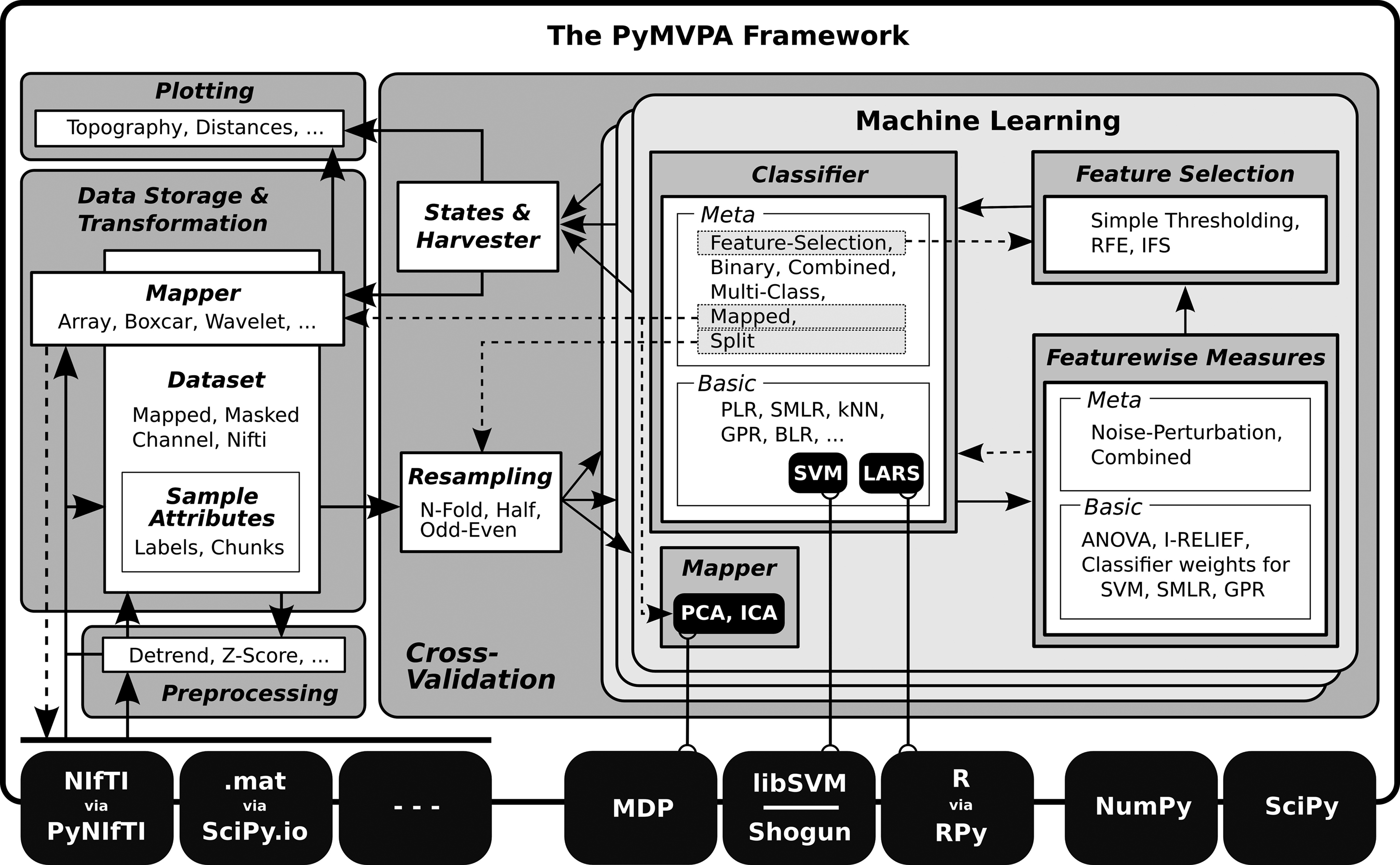
Figure 1. PyMVPA workflow and design. PyMVPA is a modular framework. It consists of several components (gray boxes) such as ML algorithms or dataset storage facilities. Each component contains one or more modules (white boxes) providing a certain functionality, e.g., classifiers, but also feature-wise measures (e.g., I-RELIEF; Sun, 2007
), and feature selection methods (recursive feature elimination, RFE; Guyon and Elisseeff, 2003
; Guyon et al., 2002
). Typically, all implementations within a module are accessible through a uniform interface and can therefore be used interchangeably, i.e., any algorithm using a classifier can be used with any available classifier implementation, such as support vector machine (SVM; Vapnik, 1995
), or sparse multinomial logistic regression (SMLR; Krishnapuram et al., 2005
). Some ML modules provide generic meta algorithms that can be combined with the basic implementations of ML algorithms. For example, a Multi-Class meta classifier provides support for multi-class problems, even if an underlying classifier is only capable to deal with binary problems. Additionally, most of the components in PyMVPA make use of some functionality provided by external software packages (black boxes). In the case of SVM, classifiers are interfaced to the implementations in Shogun or LIBSVM. PyMVPA only provides a convenience wrapper to expose them through a uniform interface. By providing simple, yet flexible interfaces, PyMVPA is specifically designed to connect to and use externally developed software. Any analysis built from those basic elements can be cross-validated by running them on multiple dataset splits that can be generated with a variety of data resampling procedures (e.g., bootstrapping, Efron and Tibshirani, 1993
). Detailed information about analysis results can be queried from any building block and can be visualized with various plotting functions that are part of PyMVPA, or can be mapped back into the original data space and format to be further processed by specialized tools (i.e., to create an overlay volume analogous to a statistical parametric mapping). The solid arrows represent a typical connection pattern between the modules. Dashed arrows refer to additional compatible interfaces which, although potentially useful, are not necessarily used in a standard processing chain.
This article does not aim to provide a detailed description of the PyMVPA framework, and therefore only a rough overview about the most important technical aspects is presented here. However, a comprehensive introduction is available in Hanke et al. (2009) and the PyMVPA manual (Hanke et al., 2008
).
In PyMVPA, each building block (e.g., all classifiers) follows a simple, standardized, interface. This allows one to use various types of classifiers interchangeably, without additional changes in the source code, and makes it easy to test the performance of newly developed algorithms on one of the many didactical neuroscience-related examples and datasets that are included in PyMVPA. In addition, any implementation of an analysis method/algorithm benefits from the basic house-keeping functionality done by the base classes, reducing the necessary amount of code needed to contribute a new fully-functional algorithm. PyMVPA takes care of hiding implementation-specific details, such as a classifier algorithm provided by an external C++ library. At the same time it tries to expose all available information (e.g., classifier training performance) through a consistent interface (for reference, this interface is called states in PyMVPA).
PyMVPA makes use of a number of external software packages, including other Python modules and low-level libraries (e.g., LIBSVM
16
) and computing environments (e.g., R
17
). Using externally developed software instead of reimplementing algorithms has the advantage of a larger developer and user base and makes it more likely to find and fix bugs in a software package to ensure a high level of quality. However, using external software also carries the risk of breaking functionality when any of the external dependencies break. To address this problem PyMVPA utilizes an automatic testing framework performing various types of tests ranging from unittests (currently covering 84% of all lines of code) to sample code snippet tests in the manual and the source code documentation itself to more evolved “real-life” examples. This facility allows one to test the framework within a variety of specific settings, such as the unique combination of program and library versions found on a particular user machine.
At the same time, the testing framework also significantly eases the inclusion of code by a novel contributor by catching errors that would potentially break the project’s functionality. Being open-source does not always mean easy to contribute due to various factors such as a complicated application programming interface (API) coupled with undocumented source code and unpredictable outcomes from any code modifications (bug fixes, optimizations, improvements). PyMVPA welcomes contributions, and thus, addresses all the previously mentioned points:
Accessibility of source code and documentation: All the source code (including website and examples) together with the full development history is publicly available via a distributed version control system
18
which makes it very easy to track the development of the project, as well as to develop independently and to submit back into the project.
Inplace code documentation: Large parts of the source code are well documented using reStructuredText
19
, a lightweight markup language that is highly readable in source format as well as being suitable for automatic conversion into HTML or PDF reference documentation. In fact, Ohloh.net
20
source code analysis judges PyMVPA as having “extremely well-commented source code.”
Developer guidelines: A brief summary defines a set of coding conventions to facilitate uniform code and documentation look and feel. Automatic checking of compliance to a subset of the coding standards is provided through a custom PyLint
21
configuration, allowing early stage minor bug catching.
Moreover, PyMVPA does not raise barriers by being limited to specific platforms. It could fully or partially be used on any platform supported by Python (depending on the availability of external dependencies). However, to improve the accessibility, we provide binary installers for Windows, and MacOS X, as well as binary packages for Debian GNU/Linux (included in the official repository), Ubuntu, and a large number of RPM-based GNU/Linux distributions, such as OpenSUSE, RedHat, CentOS, Mandriva, and Fedora. Additionally, the available documentation provides detailed instructions on how to build the packages from source on many platforms.
A final important feature of PyMVPA is that it allows, by design, researchers to compress complex analyses into a small amount of code. This makes it possible to complement publications with the source code actually used to perform the analysis as Supplementary Material. Making this critical piece of information publicly available allows for in-depth reviews of the applied methods on a level well beyond what is possible with verbal descriptions. To demonstrate this feature, this paper is accompanied by the full source code to perform all analyses shown in the following sections.
In this section we provide example analyses of four datasets, each from a different modality (EEG, MEG, fMRI, and extracellular recordings). All examples follow the same basic analysis pipeline: initial modality-specific preprocessing, application of ML methods, and visualization of the results. For the modality-independent machine learning stage, all four examples employ the same analysis with exactly the same source code. Specifically, we first perform cross-validation with one or more classifiers on each dataset then compute feature-wise sensitivity measures. These measures can then be examined to reveal their implications in terms of the underlying research question.
These examples do not aim to provide an overview of the full functionality available within PyMVPA, but rather to show that ML methods can be easily applied to various types of data to provide meaningful and even thought-provoking results.
EEG
The dataset used for the EEG example consists of a single participant from a previously published study on object recognition (Fründ et al., 2008
). In the experiment, participants indicated, for a sequence of images, whether they considered each particular image a meaningful object or just object-like with a meaningless configuration. This task was performed for two sets of stimuli with different statistical properties and under two different speed constraints. EEG was recorded from 31 electrodes at a sampling rate of 500 Hz using standard recording techniques. Details of the recording procedure can be found in Fründ et al. (2008
). A detailed description of the stimuli can be found in Busch et al. (2006
, colored images) and in Herrmann et al. (2004
, line-art pictures).
Fründ et al. (2008)
performed a wavelet-based time-frequency analyses of channels from a posterior region of interest (ROI) (i.e., no multivariate methods were employed). Here, we apply multivariate methods to differentiate between two conditions: trials with colored stimuli (broad spectrum of spatial frequencies and a high level of detail) and trials with black and white line-art stimuli (Figure 2
A), collapsing the data across all other conditions. This discrimination is orthogonal to the participants task of indicating object vs. non-object stimuli.
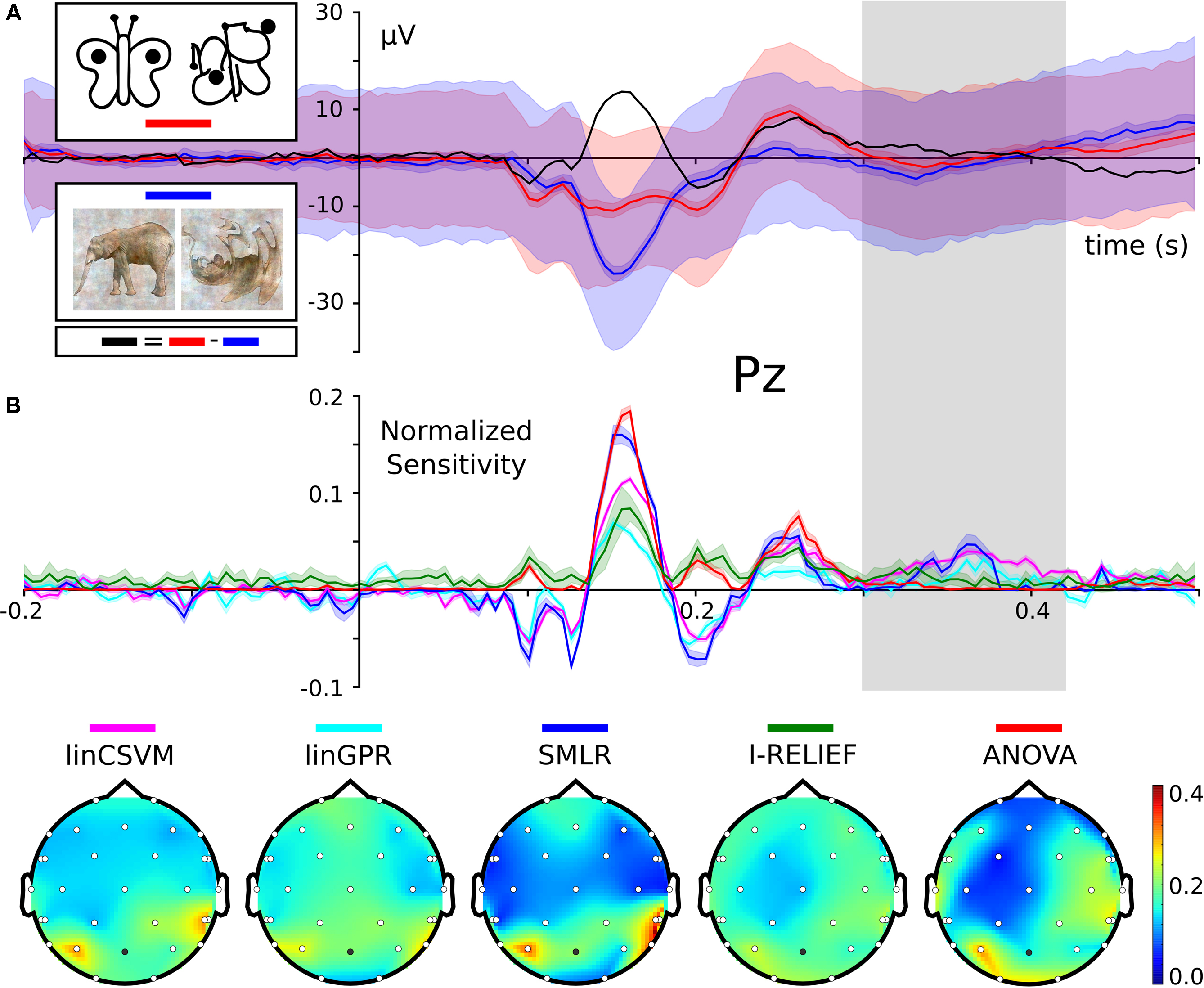
Figure 2. Sensitivities for the classification of color and line-art conditions. Panel (A) shows ERPs of each condition for electrode Pz. The light shaded area shows the standard deviation, the darker shade the 95% confidence interval around the mean ERP of each condition. The black curve is the difference wave of both ERPs. The stimulus example images are from Fründ et al. (2008)
. Panel (B) shows feature sensitivity measures for the different methods. Sensitivities were normalized by scaling the vector norm of each sensitivity vector (covering all timepoints from all electrodes) to unit length. This allows for comparison of the relative weight each classifier puts on each feature. The head topography plots in the lower panel show the channel-wise sum over time of the absolute scaled sensitivities. The upper panel shows the same scaled sensitivities plotted over time for the Pz electrode (indicated as the dark dot on the head topographies). This electrode was chosen as Fründ et al. (2008)
made it the subject of most visualizations. The shape of the sensitivity curves nicely resemble the ERP difference wave. Interestingly, for a time window around 350 ms after stimulus onset (indicated by the gray bar), all multivariate sensitivity measures assign a considerable amount of weight on the respective timepoints, whereas the univariate ANOVA is completely flat at zero.
The data for this analysis were 700 ms EEG segments starting 200 ms prior to the stimulus onset of each trial, to which we applied the following preprocessing procedure. We only included trials that passed the semi-automatic artifact rejection procedure performed in the original study, yielding 852 trials (422 color and 430 line-art). Each trial timeseries was downsampled to 200 Hz, leaving 140 sample points per trial and electrode. We then defined each trial, including the EEG signal of all sample points from all channels, as a sample to be classified (4340 features total). Finally, all features for each sample were normalized to zero mean and unit variance (z-scored).
As the main analysis we applied a standard sixfold cross-validation
22
procedure with linear support vector machine (linCSVM; Vapnik, 1995
), sparse multinomial logistic regression (SMLR; Krishnapuram et al., 2005
) and Gaussian process regression with linear kernel (linGPR; Rasmussen and Williams, 2006
) classifiers. Additionally, we computed the multivariate I-RELIEF (Sun, 2007
) feature sensitivity measures, and, for comparison, a univariate analysis of variance (ANOVA) F-score on the same cross-validation dataset splits.
All three classifiers performed with high accuracy on the independent test datasets, achieving 86.2% (linCSVM), 91.8% (SMLR), and 89.6% (linGPR) correct single trial predictions, respectively. However, more interesting than the plain accuracy are the features each classifier relied upon to perform its predictions. PyMVPA makes it very easy to extract feature sensitivity information from all its classifiers using a uniform interface. Figure 2
B shows the computed sensitivities from all classifiers and measures. There is a striking similarity between the shape of the classifier sensitivities plotted over time and the corresponding event-related potential (ERP) difference wave between the two experimental conditions (Figure 2
A; example shown for electrode Pz, Fründ et al., 2008
). The head topography plot of the sensitivities reveals a high variability with respect to the specificity among the multivariate measures. SVM, GPR and SMLR weights congruently identify three posterior electrodes as being most informative (SMLR weights provide the highest contrast of all measures). The I-RELIEF topography is much less specific and more similar to the ANOVA topography in its global spatial structure than to the other multivariate measures. It should be noted, however, that these topographies aggregate information over all timepoints and, therefore, do not provide information about specific temporal EEG components.
One particularly interesting result is the difference between the multivariate sensitivities and the univariate ANOVA F-scores from 300 to 400 ms following stimulus onset. Only the multivariate methods (especially SMLR, linCSVM and linGPR) detected a relevant contribution to the classification task of the signal in this time window. This late signal may be related to the intracranial EEG gamma-band responses that Lachaux et al. (2005)
observed at around the same time range when participants viewed complex stimuli. Given that the present data also seem to show a similar evoked gamma-band response (Fründ et al., 2008
), it is possible that the multivariate methods are sensitive to the gamma-band activity in the data. Still, further work would be required to prove this correlation.
MEG
The example MEG dataset was collected with the aim to test whether it is possible to predict the recognition of briefly presented natural scenes from single trial MEG-recordings of brain activity (Rieger et al., 2008
) and to use ML methods to investigate the properties of the brain activity that is predictive of later recognition. On each trial participants saw a briefly presented photograph (37 ms) of a natural scene that was immediately followed by a pattern mask (1000–1400 ms). The short masked presentation effectively limits the processing interval of the scene in the brain (Rieger et al., 2005
) and, therefore, participants will later recognize only some of the scenes. After the mask was turned off, participants indicated via button presses whether they would subsequently recognize the photograph, or if they would fail. Immediately after this judgement, four natural scene photographs were presented and participants had to indicate which of the four scenes had been previously presented (i.e., a four-alternative forced-choice delayed match to sample task).
The MEG was recorded with a 151 channel CTF Omega MEG system from the whole head (sampling rate 625 Hz and a 120 Hz analogue low pass filter) while participants performed this task. The 600 ms interval of the MEG time series data that was used for the analysis started at the onset of the briefly presented scene and ended before the mask was turned off. As in the original study, we analyzed only those trials in which participants both judged they would be correct and also correctly recognized the scene (RECOG) and the trials in which participants both predicted they would fail and gave an incorrect response (NRECOG). For details about the rationale of this selection, the stimulus presentation information, and the recording procedure see Rieger et al. (2008)
. In this example analysis we have used data from a single participant (labeled P1 in the original publication).
The MEG timeseries were first downsampled to 80 Hz and then all trial segments were channel-wise normalized by subtracting their mean baseline signal (determined from a 200 ms window prior to scene onset). Only timepoints within the first 600 ms after stimulus onset were considered for further analysis. The resulting dataset consisted of 151 channels with 48 timepoints each (7248 features), and a total of 294 samples (233 RECOG trials and 61 NRECOG trials).
The original study contained analyses based upon SVM classifiers, which revealed, by means of the spatio-temporal distribution of the sensitivities, that the theta band alone provides the most discriminative signal. The authors also addressed the topic of how to interpret heavily unbalanced datasets
23
. Given this comprehensive analysis, we aimed here to replicate their basic analysis strategy with PyMVPA and were able to achieve almost identical results.
As with the EEG data, we applied a standard cross-validation procedure, this time eightfold, using linear SVM and SMLR classifiers. Additionally, we again computed univariate ANOVA F-scores on the same cross-validation dataset splits. The SVM classifier was configured to use different per-class C-values
24
, scaled with respect to the number of samples in each class to address the unbalanced number of samples. Similar to Rieger et al. (2008)
, we also ran a second cross-validation on balanced datasets (by performing multiple selections of a random subset of samples from the larger RECOG category).
Both, classifiers performed almost identically on the full, unbalanced dataset, achieving 84.69% (SMLR) and 82.31% (linCSVM) correct single trial predictions (83.0% in the original study). Figure 3
shows sample timeseries of the classifier sensitivities and the ANOVA F-score of two posterior channels. Due to the significant difference in the number of samples of each category, it is important to additionally report mean true positive rate (TPR)
25
, that amounted to 72% (SMLR), and 76% (linCSVM) respectively. The second SVM classifier trained on the balanced dataset achieved a comparable accuracy of 76.07% correct predictions (mean across 100 subsampled datasets), which is a slightly larger drop in accuracy when compared to the 80.8% achieved in the original study (see Table 3 in Rieger et al., 2008
).
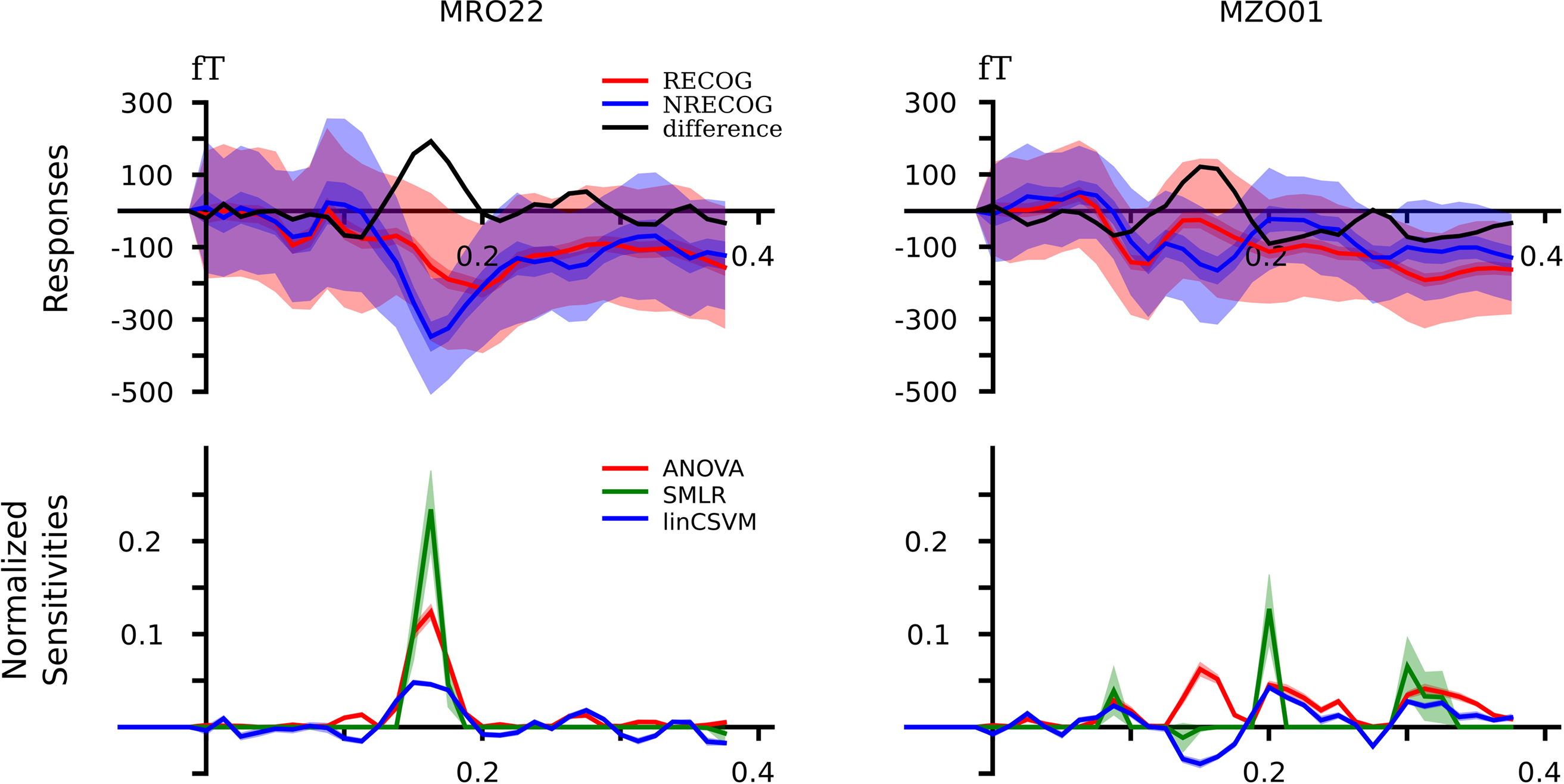
Figure 3. Event-related magnetic fields (EMF) and classifier sensitivities. The upper part shows EMFs for two exemplary MEG channels. On the left sensor MRO22 (right occipital), and on the right sensor MZO01 (central occipital). The lower part shows classifier sensitivities and ANOVA F-scores plotted over time for both sensors. Both classifiers showed equivalent generalization performance of approximately 82% correct single trial predictions.
Importantly, these results show that PyMVPA produces reproducible results that depend on the ML methods employed, but not on a particular implementation. However, the integrated framework of PyMVPA allowed us to achieve these results with much less effort than what was necessary in the original study.
fMRI
A single participant (participant 1) from a study published by Haxby et al. (2001)
, which has been repeatedly reanalyzed since the original publication (Hanson and Halchenko, 2008
; Hanson et al., 2004
; O’Toole et al., 2007
), served as the example fMRI dataset. The dataset itself consists of 12 runs. In each run, the participant passively viewed greyscale images of eight object categories, grouped in 24 s blocks separated by rest periods. Each image was shown for 500 ms and was followed by a 1500 ms inter-stimulus interval. Full-brain fMRI data were recorded with a volume repetition time of 2500 ms, thus, a stimulus block was covered by roughly nine volumes. For a complete description of the experimental design and fMRI acquisition parameters see Haxby et al. (2001)
.
First, the raw fMRI data were motion corrected using FLIRT
26
from FSL
27
(Jenkinson et al., 2002
). All subsequent data processing was done with PyMVPA. After motion correction, linear detrending was performed for each run individually. No additional spatial or temporal filtering was applied.
For the sake of simplicity, we reduced the dataset to a four-class problem (faces, houses, cats, and shoes). All volumes recorded during any of these blocks were extracted and voxel-wise z-scored. This normalization was performed individually for each run to prevent any kind of information transfer across runs.
After preprocessing, we applied the same sensitivity analysis performed for all other data modalities to this dataset. Here, only a SMLR classifier was used (sixfold cross-validation, with 2 of the 12 experimental runs grouped into one chunk, and trained on single fMRI volumes that covered the full brain). For comparison, a univariate ANOVA was again computed for the same cross-validation dataset splits.
The SMLR classifier performed very well on the independent test datasets, correctly predicting the category for 94.7% of all single volume samples in the test datasets. To examine what information was used by the classifier to reach this performance level, we computed ROI-based sensitivity scores for 48 non-overlapping structures defined by the probabilistic Harvard-Oxford cortical atlas (Flitney et al., 2007
), as shipped with FSL (Smith et al., 2004
). To create the ROIs, we thresholded the probability maps of all structures at 25% and assigned ambiguous voxels to the structure with the higher probability. The resulting map was projected into the space of the functional dataset using an affine transformation and nearest neighbor interpolation.
In order to determine the contribution of each ROI, the sensitivity vector was first normalized (across all ROIs), so that all absolute sensitivities summed up to 1 (L1-normed). Afterwards ROI-wise scores were computed by taking the sum of all sensitivities in a particular ROI. The upper part of Figure 4
shows these scores for the 20 highest-scoring and the three lowest-scoring ROIs.
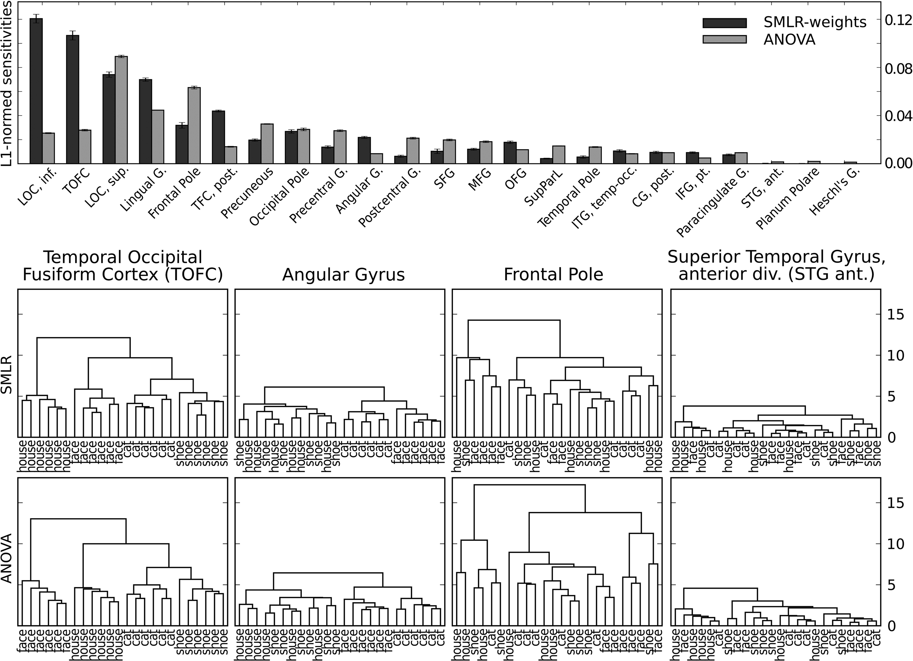
Figure 4. Sensitivity analysis of the four-category fMRI dataset. The upper part shows the ROI-wise scores computed from SMLR classifier weights and ANOVA F-scores (limited to the 20 highest and the three lowest-scoring ROIs). The lower part shows dendrograms with clusters of average category samples (computed using squared Euclidean distances) for voxels with non-zero SMLR-weights and a matching number of voxels with the highest F-scores in each ROI.
The lower part of the figure shows dendrograms from a hierarchical cluster analysis
28
on relevant voxels from a block-averaged variant of the dataset (but otherwise identical to the classifier training data). For SMLR, only voxels with a non-zero sensitivity were considered in each particular ROI. For ANOVA, only the voxels with the highest F-scores (limited to the same number as for the SMLR case) were considered. For visualization purposes the dendrograms show the distances and clusters computed from the average samples of each condition in each dataset chunk (i.e., two experimental blocks), yielding six samples per condition.
The four chosen ROIs clearly show four different cluster patterns. The 92 selected voxels in temporal occipital fusiform cortex (TOFC) show a clear clustering of the experimental categories, with relatively large sample distances between categories. The pattern of the 36 voxels in angular gyrus reveals an animate/inanimate clustering, although with much smaller distances. The largest group of 148 voxels in the frontal pole ROI seems to have no obvious structure in their samples. Despite that, both sensitivity measures assign substantial importance to this region. This might be due to the large inter-sample distances visualized in the corresponding dendrogram in Figure 4
. Each leaf node (in this case an average volume of two stimulation blocks) is approximately as distinct from any other leaf node, in terms of the employed distance measure, as the semantic clusters identified in the TOFC ROI. Finally, the ROI covering the anterior division of the superior temporal gyrus shows no clustering at all, and, consequently, is among the lowest-scoring ROIs of both measures. On the whole, the cluster patterns from voxels selected by SMLR weights and F-scores are very similar in terms of inter-cluster distances.
Given that these results only include the data of a single participant, no far-reaching implications can be drawn from them. However, the distinct cluster patterns might provide indications for different levels of information encoding that could be addressed in future studies. Although voxels selected in both angular gyrus and the frontal pole ROIs do not provide a discriminative signal for all four stimulus categories, they nevertheless provide some disambiguating information and, thus, are picked up by the classifier. In angular gyrus, this seems to be an animate/inanimate pattern that additionally also differentiates between the two categories of animate stimuli. Finally, in the frontal pole ROI the pattern remains unclear, but the relatively large inter-sample distances indicate a differential code of some form that is not closely related to the semantic stimulus category.
Extracellular Recordings
The extracellular dataset analyzed in this section is previously unpublished, thus, we first briefly describe the experimental and acquisition setup. Animal experiments were carried out in accordance with the National Institute of Health Guide for the Care and Use of Laboratory Animals and approved by Rutgers University. Sprague-Dawley rats (300–500 g) were anaesthetized with urethane (1.5 g/kg) and held with a custom naso-orbital restraint. After preparing a 3 mm square window in the skull over auditory cortex, the dura was removed and a silicon microelectrode consisting of eight four-site recording shanks (NeuroNexus Technologies, Ann Arbor, MI, USA) was inserted. The recording sites were in the primary auditory cortex, estimated by stereotaxic coordinates, vascular structure (Sally and Kelly, 1988
) and tonotopic variation of frequency tuning across recording shanks, and located within layer V, determined by electrode depth and firing patterns.
Five pure tones (3, 7, 12, 20, 30 kHz at 60 dB) and five different natural sounds (extracted from the CD “Voices of the Swamp”, Naturesound Studio, Ithaca, NY, USA) were used as stimuli. Each stimulus had a duration of 500 ms followed by 1500 ms of silence. All stimuli were tapered at beginning and end with a 5 ms cosine window. The data acquisition took place in a single-walled sound isolation chamber (IAC, Bronx, NY, USA) with sounds presented free field (RP2/ES1, Tucker-Davis, Alachua, FL, USA).
Individual units
29
were isolated by a semi-automatic algorithm (KlustaKwik
30
) followed by manual clustering (Klusters
31
). Post-stimulus time histograms (PSTH) of spike counts per each unit for all 1734 stimulation onsets were estimated using a bin size of 3.2 ms. To ensure an accurate estimation of PSTHs only units with a mean firing rate higher than 2 Hz were selected for further analysis, leaving us with a total of 105 units.
Since the segregation of individual units out of the extracellular recordings is carried out without taking the respective stimulus condition into account, i.e., in unsupervised fashion (in ML terminology), it does not guarantee that the activity of any particular unit can be easily attributed to some set of stimulus conditions. From the stimulus-wise descriptive statistics of the units presented in the top plots of Figure 5
it is difficult to state that the activity of any particular unit at some moment in time is specific for a given stimulus. Furthermore, due to the inter-trial variance in the spike counts, it is even more difficult to reliably assess what stimulus condition any particular trial belongs to. Hence, the purpose of the PyMVPA analysis was to complement the results of the unsupervised clustering with a characterization of all extracted units in terms of their specificity to any given stimulus at any given time.
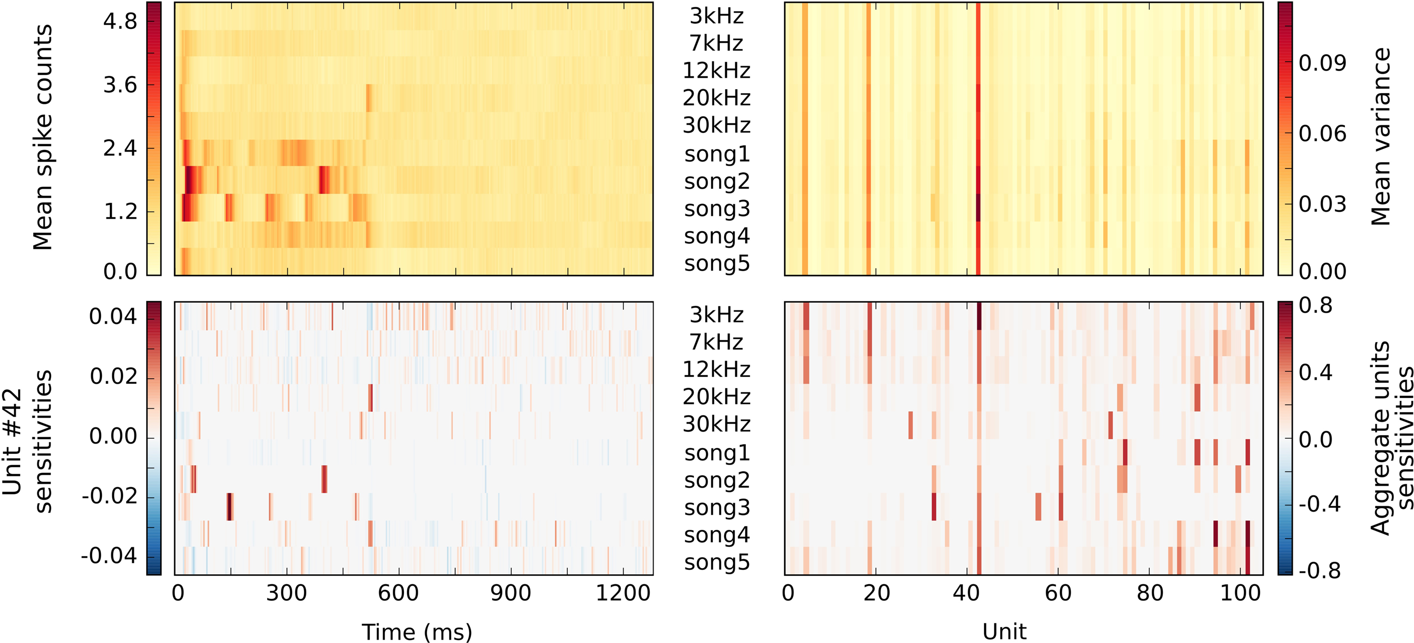
Figure 5. Statistics of multiple single unit extracellular simultaneous recordings and corresponding classifier sensitivities. All plots sweep through different stimuli along vertical axis, with stimuli labels presented in the middle of the plots. The upper part shows basic descriptive statistics of spike counts for each stimulus per each time bin (on the left) and per each unit (on the right). Such statistics seem to lack stimulus specificity for any given category at a given time point or unit. The lower part on the left shows the temporal sensitivity profile of a representative unit for each stimulus. It shows that stimulus specific information in the response can be coded primarily temporally (few specific offsets with maximal sensitivity like for song2 stimulus) or in a slowly modulated pattern of spikes counts (see 3 kHz stimulus). Associated aggregate sensitivities of all units for all stimuli in the lower right figure indicate each unit’s specificity to any given stimulus. It provides better specificity than simple statistics like variance, e.g., unit 19 is active in all stimulation conditions according to its high variance, but according to its classifier sensitivity it carries little, if any, stimuli-specific information for natural songs 1–3.
The analysis pipeline was similar to the one used for EEG, MEG, and fMRI data. We ran a standard eightfold cross-validation procedure for an SMLR classifier, which achieved a mean of 77.57% accuracy estimate across all 10 types of stimuli. This generalization accuracy is well above chance (10%) for all stimulus categories and allows one to conclude that the neuronal population activity pattern at the recording site carries a differential signal across all 10 stimuli. Misclassifications mostly occurred for low-frequency stimuli. Pure tones with 3 and 7 kHz were more often confused with each other than tones with a larger frequency difference (see Figure 6
), which suggests a high similarity in the spiking patterns for these stimuli. We could further speculate that this neuronal population is more tuned towards the processing of higher frequency tones.
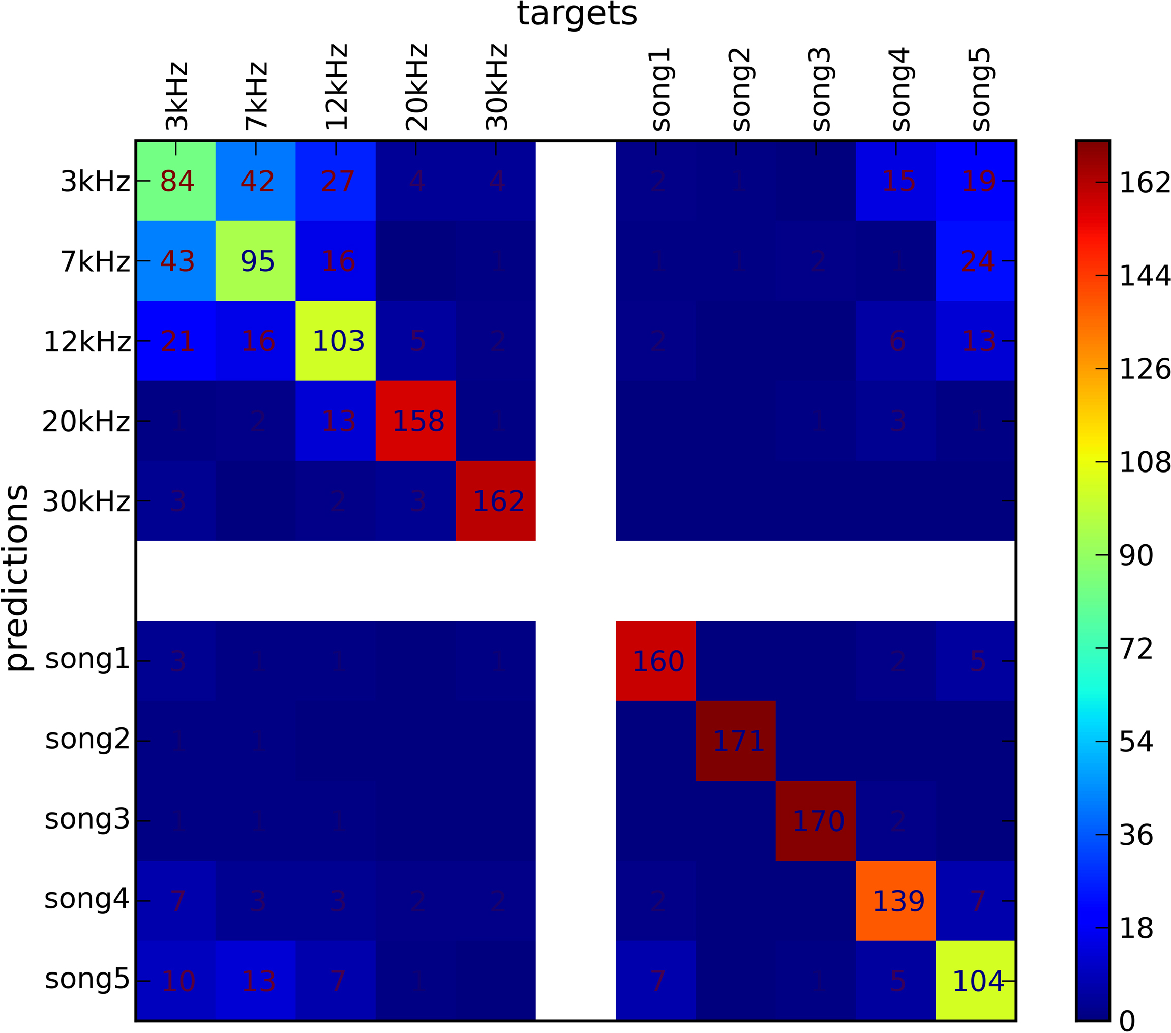
Figure 6. Confusion matrix of SMLR classifier predictions of stimulus conditions from of multiple unit recordings. The classifier was trained to discriminate between stimuli of five pure tones and five natural sounds. Elements of the matrix (numeric values and color-mapped visualization) show the number of trials which were correctly (diagonal) or incorrectly (off-diagonal) classified by a SMLR classifier during an eightfold cross-validation procedure. The results suggest a high similarity in the spiking patterns for stimuli of low-frequency pure tones, which lead the classifier to confuse them more often, whenever responses to natural sound stimuli and high-frequency tones were hardly ever confused with each other.
Besides being able to label yet unseen trials with high accuracy, the trained classifier can readily provide its sensitivity estimates for each unit, time bin, and stimulus condition (see bottom plots of Figure 5
). Temporal sensitivity profiles of any particular unit (see unit #42 profiles in lower left plot of Figure 5
) can reveal that the stimulus specific information is contained in spike times relative to stimulus onset or can be represented as slowly modulated pattern of spike counts (see 3 kHz stimuli). An aggregate sensitivity (in this case the sum of absolute sensitivities) across all time-bins provides a summary statistic of any unit’s sensitivity to a given stimulus condition (see lower right plot of Figure 5
). In contrast to a simple variance measure, it provides an easier way to associate any given unit to a set of stimulus conditions. Additionally, it can identify units which might lack a substantial amount of variance, but nevertheless carry a stimulius-specific signal (e.g. unit #28 and 30 kHz stimulus).
In this article we presented PyMVPA, a data analysis framework especially tailored to neural data from a wide range of acquisition modalities. PyMVPA provides ML techniques as core functionality, addressing recent trends in neuroscience research. To illustrate the generalizability of the PyMVPA analysis pipeline we provided example analyses of data from EEG, MEG, fMRI and extracellular recordings.
The framework presented here is Python-based, sophisticated, free and open-source software. Its intended audience is threefold. First, there are neuroscience researchers interested in testing ML algorithms on neural data, e.g., people working on brain-computer interfaces (BCI, see Birbaumer and Cohen, 2007
; Lebedev and Nicolelis, 2006
). PyMVPA provides researchers with the ability to execute complex analysis tasks in very concise code. Second, it is also designed for ML researchers interested in testing new ML algorithms on neural data. PyMVPA offers a highly-modularized architecture designed to minimize the effort of adding new algorithms. Moreover, the availability of neuroscience-related code-examples (like the ones presented in this article) and datasets greatly reduces the time to get actual results. Finally, PyMVPA is welcoming code contributors from both neuroscience and ML communities interested in improving or adding modality-specific functions or new algorithms. PyMVPA offers a community-based development model together with a distributed version control system and extensive reference documentation.
Future Work
PyMVPA does not aim to provide all possible ML analysis algorithms, and it will likely not come close, even in the future. Given that PyMVPA is tailored towards the high-dimensional problems found in neuroscience, it currently provides many of the most common algorithms tuned for this target. Still, as the neuroscience and ML communities unite, new and promising algorithms are constantly emerging and being added to PyMVPA. Beyond the inclusion of new ML algorithms, there are numerous plans for future enhancements to PyMVPA.
Because the current use of ML techniques in neuroscience is mainly limited to the application of only basic algorithms to neural data, one of the next, most intriguing, new directions of PyMVPA will be to provide custom workflows designed for specific neuroscience modalities. An example of such a custom workflow is the analysis of fMRI data from experiments with event-related designs, where multiple fMRI volumes after the onset of the event compose a single sample within a dataset provided to the ML methods for processing. Combining multiple volumes into a single sample obviates the need to provide a hemodynamic response function because the important features can be extracted independently for each voxel.
In addition, PyMVPA has yet to confront the problem of model selection. Currently, only Gaussian process regression has the ability to select hyper-parameters of the model. Uniform model selection for ML methods within PyMVPA is planned for the next major release of the project. It will provide the facility to automatically search for the best set of parameters for each classifier without sacrificing unbiased estimates of the generalization performance.
The Supplemental Materials (e.g., source code) for this article can be found online at http://www.frontiersin.org/neuroinformatics/paper/10.3389/neuro.11/003.2009.
The authors declare that the research was conducted in the absence of any commercial or financial relationships that could be construed as a potential conflict of interest.
We are thankful to Dr. Artur Luczak and Dr. Kenneth D. Harris (CMBN, Rutgers University, Newark, NJ, USA) for providing the extracellular recordings dataset for the paper. Michael Hanke was supported by the German Academic Exchange Service (grant: PPP-USA D/05/504/7). Per Sederberg was supported by National Institutes of Health NRSA (grant: MH080526). Yaroslav O. Halchenko and Dr. Stephen J. Hanson were supported by the National Science Foundation (grant: SBE 0751008) and the James McDonnell Foundation (grant: 220020127). Stefan Pollmann and Jochem W. Rieger were supported by Deutsche Forschungsgemeinschaft (PO 548/6-1 and RI 1511/1-3 respectively).
- ^ Electroencephalography.
- ^ Magnetoencephalography.
- ^ Magnetic resonance imaging.
- ^ Positron emission tomography.
- ^ http://www.mloss.org .
- ^ Closed source commercial product of MathWorks®.
- ^ It is possible to use the low-level functions of this toolbox for other modalities.
- ^ http://numpy.scipy.org .
- ^ http://www.scipy.org .
- ^ e.g., ctypes, SWIG, SIP, Cython.
- ^ e.g., mlabwrap and RPy.
- ^ http://www.pymvpa.org .
- ^ http://mdp-toolkit.sourceforge.net .
- ^ http://code.google.com/p/scipy-cluster/ .
- ^ PyMVPA is distributed under an MIT license, which complies with both Free Software and Open Source definitions.
- ^ http://www.csie.ntu.edu.tw/ ∼cjlin/libsvm/ .
- ^ http://www.r-project.org .
- ^ http://en.wikipedia.org/wiki/Version_control_system .
- ^ http://en.wikipedia.org/wiki/ReStructuredText .
- ^ http://www.ohloh.net/projects/pymvpa/factoids .
- ^ http://www.logilab.org/projects/pylint .
- ^ http://en.wikipedia.org/wiki/Cross-validation#K-fold_cross-validation .
- ^ Unbalanced datasets have a dominant category which has considerably more samples than any other category. That potentially leads to the problem when a classifier prefers to assign the label of that category to all samples to minimize total prediction error.
- ^ Parameter C in soft-margin SVM controls a trade-off between width of the SVM margin and number of support vectors (see Veropoulos et al., 1999, for an evaluation of this approach).
- ^ Mean TPR is equivalent to accuracy in balanced sets, and is 50% at chance performance even with unbalanced set sizes (see Rieger et al., 2008, for a discussion of this point).
- ^ FMRIB’s Linear Image Registration Tool.
- ^ http://www.fmrib.ox.ac.uk/fsl .
- ^ PyMVPA provides hierarchical clustering facilities through hcluster (Eads, 2008).
- ^ The term “unit” in the text refers to a single entity, which was segregated from the recorded data, and is expected to represent a single neuron.
- ^ http://klustakwik.sourceforge.net .
- ^ http://klusters.sourceforge.net .
Detre, G., Polyn, S. M., Moore, C., Natu, V., Singer, B., Cohen, J., Haxby, J. V., and Norman, K. A. (2006). The Multi-Voxel Pattern Analysis (MVPA) Toolbox. Poster presented at the Annual Meeting of the Organization for Human Brain Mapping (Florence, Italy). Available at: http://www.csbmb.princeton.edu/mvpa
.
Eads, D. (2008). Hcluster: Hierarchical Clustering for SciPy. Available at: http://scipy-cluster.googlecode.com/
.
Flitney, D., Webster, M., Patenaude, B., Seidman, L., Goldstein, J., Tordesillas Gutierrez, D., Eickhoff, S., Amunts, K., Zilles, K., Lancaster, J., Haselgrove, C., Kennedy, D., Jenkinson, M., and Smith, S. (2007). Anatomical Brain Atlases and Their Application in the FSLView Visualisation Tool. Thirteenth Annual Meeting of the Organization for Human Brain Mapping. Chicago, IL, USA.
Hanke, M., Halchenko, Y. O., Sederberg, P. B., and Hughes, J. M. (2008). The PyMVPA Manual. Available at: http://www.pymvpa.org/PyMVPA-Manual.pdf
.
Smith, S. M., Jenkinson, M., Woolrich, M. W., Beckmann, C. F., Behrens, T. E. J., Johansen-Berg, H., Bannister, P. R., De Luca, M., Drobnjak, I., Flitney, D. E., Niazy, R. K., Saunders, J., Vickers, J., Zhang, Y., De Stefano, N., Brady, J. M., and Matthews, P. M. (2004). Advances in functional and structural MR image analysis and implementation as FSL. Neuroimage 23, 208–219.
Sonnenburg, S., Braun, M., Ong, C. S., Bengio, S., Bottou, L., Holmes, G., LeCun, Y., Müller, K.-R., Pereira, F., Rasmussen, C. E., Rätsch, G., Schölkopf, B., Smola, A., Vincent, P., Weston, J., and Williamson, R. (2007). The need for open source software in machine learning. J. Mach. Learn. Res. 8, 2443–2466.