Finite element analysis of cardiovascular stent frames: identifying appropriate mesh discretization

Engineers use finite element analysis (FEA) to predict the deformations, strains, stresses, and resistive forces of metallic stent frames under in vivo, in vitro, and manufacturing-induced loading conditions. The discretization of the geometric model influences the simulation predictions, with the error generally reducing with mesh refinement. This improved accuracy comes with the trade-off of requiring more resources. Since FEA influences decisions that carry patient and business risk, engineers must balance the computational cost against numerical accuracy. This paper explores a methodology for selecting the mesh discretization for a computational model of an implantable stent frame based on discretization error, computational cost, and the risk associated with using the model to inform a specific decision. The methodology includes estimating the exact solution for the numerical model, calculating the discretization error and computational cost for various mesh discretization options, and considering the error and cost when selecting one of the options. The method was applied to a laser-cut nitinol stent model for four different finite element solvers to demonstrate its real-world applicability and that it is agnostic to solver type and developer. We were able to estimate the exact solution to the numerical model with a 95% confidence interval using submodeling, a geometry representative of the full stent frame, and four systematically refined meshes. The selection of the mesh discretization is subjective, with the importance of each model’s computational cost dependent on the number of simulations, resource availability, and risk. Three real-world implantable medical device examples of using FEA to inform a project decision are presented, each with a mesh discretization option suggested and rationalized based on the discretization error and computational costs. FEA’s important role in developing implantable stent frames and providing evidence of their safety to decision makers and regulatory bodies underscores the need for a method to select a suitable mesh discretization. The methodology explored in this paper calculates the error in the model’s prediction due to discretization and the computational cost. A project team can use this information and the risk associated with using the model to select and rationalize a specific mesh discretization.

1 Introduction

Metallic frames constitute or are a component of many endoscopically delivered implantable medical devices, including coronary stents, atrial appendage occluders, and vena cava filters. A subset of implantable metallic frames, stent frames provide structural support to the device and the surrounding tissue. In addition to cardiovascular applications, stent frames have been used to treat narrowing or obstruction of the trachea or bronchus (Walser, 2005), bile ducts (Isayama et al., 2012), and the urinary tract (Salamanca-Bustos et al., 2018). The loads experienced by the frame are dependent on the device’s application and location. A stent graft consisting of a cylindrical frame and covering may be used in the cardiovascular system to improve or redirect blood flow. For example, the GORE^® VIABAHN^® Endoprosthesis (Figure 1A), manufactured by Gore Medical, is approved in the United States for treating atherosclerotic lesions in the superficial femoral and iliac arteries. The metallic frame expands the vessel lumen, improving blood flow, and the graft covers and seals off residual thrombosis. After implantation, the pulsatile nature of blood flow and patient movement can result in multiple loading modes on stent frames, including bending, compression, and torsion. The frame must also adapt to the local curvature of the arteries, both at rest and under dynamic conditions such as walking.

Figure 1

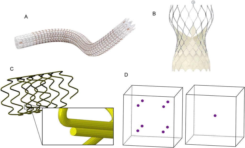
Figure 1. (A) GORE^® VIABAHN^® Endoprosthesis. ©W. L. Gore and Associates, Inc. Used with permission. (B) Medtronic Evolut™ Transcatheter Aortic Valve. ©Medtronic, PLC. Used with permission. (C) The wire-wound stent frame is discretized into hexahedral elements. (D) Integration points within hexahedral elements. The left element is fully integrated with eight integration points, and the reduced integration element on the right has one integration point at its center.

Frames may also provide structural support for a device that blocks flow or functions as a valve. Medtronic manufactures both surgically and endoscopically implanted heart valve replacements. These valves consist of a metal frame, leaflets that control blood flow, and a covering that attaches the leaflets to the frame and prevents leakage. Medtronic’s Evolut™ aortic valve bioprosthesis (Figure 1B), which is endovascularly implanted, features a nitinol frame that provides chronic outward force and a supporting structure for the valve leaflets. Its frame is flexible, enabling load sharing with the leaflets when the valve is closed, and it can return to its deployed position as the leaflets begin to open. Medical device engineers utilize finite element analysis (FEA) to predict the performance and durability of these devices during the development and assessment phases of the design process. In the case of the GORE^® VIABAHN^® Endoprosthesis and similar devices, FEA may be used to predict the device’s radial outward pressure at the indicated use diameters and the frame’s durability under multimodal loading. The Medtronic Evolut™ aortic valve development process used FEA to assess leaflet stresses when the valve is closed and the ability of the frame to resist fracture over hundreds of millions of heartbeats.

Traditional FEA solvers require the geometry to be subdivided (discretized) into elements, which are closed one, two, or three-dimensional shapes composed of points (nodes) connected by lines or curves (see Figure 1C). Each element has one or more integration points where the strain and stress are calculated. The deformation and displacement of the nodes in response to applied loads, constraints, and prescribed motion change the element’s shape, volume, and location.

Peak strain and stress in a mechanical construct occur at the surface when exposed to a bending or torsional load. A stent frame composed of connected struts or woven wire may experience diametric, torsional, and longitudinal loading when radially compressed to fit onto a deployment system and then delivered in vivo. Since mesh integration points are internal to the element (see Figure 1D), stress and strain are not calculated at the surface if the mesh is solely composed of 3-dimensional elements. Techniques such as extrapolating the output to the nodes and skinning the mesh surface with 2-dimensional elements (Sinha, 2018) are two means for compensating for the location of the 3-dimensional element integration points. Additional aspects of the discretization that may impact the computational model’s ability to predict the deformation, strain, and stress for the entire structure are the mesh’s quality (skew, aspect ratio, etc.), order (linear vs. quadratic), element size (length of element’s edge), quantity of integration points per element, and consistency of the elements.

A mesh refinement study, using consistently refined meshes, is conducted to characterize how the discretization of the mesh impacts the computational model’s prediction of the quantity of interest. Typically, stress or strain, which are calculated at the element’s integration points, are the quantity of interest for computational models of implantable metallic frames that are used to address durability-related questions. Refining a mesh, which involves a uniform reduction in element size for all elements, will improve the prediction at the integration points in the case of a bending or torsion load because these points are closer to the surface of the mesh, where peak strains and stresses occur. With each successive refinement, the differences in the quantity of interest will decrease as the integration points approach the mesh’s surface. Therefore, mesh refinement studies for a computational model of a stent frame used to predict stress or strain is limited to the values predicted at the integration points of the three-dimensional elements, and should not use values from two-dimensional elements skinned on the mesh’s surface or values extrapolated from the integration points to the nodes on the surface of the mesh.

The fractional change (ε) in the quantity of interest between successive mesh refinements, expressed as a percentage, is calculated using Equation 1 (Guler et al., 2022)

$\left|\epsilon \right|=\frac{\left|w_C-w_F\right|}{\left|w_F\right|}\ast 100(1)$

where w_C and w_F are the outputs from two mesh levels, and the element size for the C (coarse) mesh is greater than that of the F (fine) mesh. This metric has been used to identify when the output of a computational model has converged, and thus, further refinement of the mesh is unnecessary. For medical device simulations, a fractional change of 5.0% or less between the peak strain predictions is a common acceptance criterion for selecting an appropriate element size (ASTM F2996, 2020; ASTM F3334, 2019; Karanasiou et al., 2017). The rationale is that the marginal gains in accuracy outweigh the computational costs associated with further refinement. As shown by Guler et al. (2022), this can be true for specific values of the refinement factor and order of convergence. However, the 5.0% threshold is arbitrary and unrelated to the patient or business risk associated with making a decision based on the simulation results or the computational cost of the simulations. This calculation also fails to provide insight into the error and uncertainty in the prediction due to the mesh’s discretization.

Characterizing the risk associated with making a decision impacting the design or use of a medical device based on simulation results is a topic covered in detail in the ASME V&V 40 standard (ASME V&V 40, 2018). The standard refers to this as model risk, which is determined by considering the influence the simulation results have on the decision and the ramifications of making an incorrect decision. The simulation results’ influence on the decision depends on the quantity and quality of the other sources of evidence, such as bench-top testing. Making an incorrect decision can negatively impact patients and the business, with the probability and severity being options for assessing the identified harms.

The computational models whose discretization is informed by a mesh refinement study (e.g., models used for validation and to inform decisions) are not limited to reporting strains or stresses only at the integration points of the three-dimensional elements. To reduce the computational cost of the simulations, an analyst may want to incorporate a different element type than what was used in the mesh refinement study, skin the mesh surface while increasing the size of three-dimensional elements, and apply element aspect ratios (the longest edge length divided by the shortest edge length for hexahedral elements) greater than 1.0. These modifications can be easily rationalized if their impact on the model’s accuracy is known, which is impossible if the mesh refinement study only calculates fractional change.

Cost, defined as the time to run a simulation divided by the number of cores used, impacts the time required to accumulate the evidence (simulation results) needed to make a decision and the resources (computational cores, software licenses) that could be allocated to address other questions. This paper reports the computational cost of the discretization options in relative terms. For example, if the simulation is expected to take 6 h to complete when run over 24 cores using one of the discretization options, and another option has a relative computational cost that is 33% less, it can be expected that the same simulation with the less costly discretization may require ∼4 h on the same number of cores. Or ∼2 h with twice the number of cores, with the understanding that the threading of the cores, the time to write data, and other factors also influence the run time.

Understanding the error in the predicted quantity of interest and the relative computational cost enables engineers to make informed decisions when selecting an appropriate mesh discretization. This paper explores a process for calculating discretization error and computational cost for various discretization options. As an example of the process, the selection of a mesh discretization for a laser-cut nitinol stent frame under in vivo loading conditions is described in the Methods section. During the simulation, the frame is expanded, annealed, and radially compressed to 50% of its expanded outer diameter to mimic catheter loading. It is then partially released to simulate implantation into a vessel. This example is used as a vehicle for addressing multiple questions: what element type to use to estimate the exact solution, how to estimate the exact solution and discretization error, what are the final mesh discretization options, how to select a mesh discretization, and whether this process is limited to a single type or brand of FEA solver. In the Discussion section, we examine the mesh refinement results for the laser-cut nitinol stent frame across multiple contexts of use, spanning a continuum of model risk from low to high. The model risk for each is assessed based on the simulation results’ influence on the decision and the potential harm induced to patients or the business if the decision is incorrect. We select a mesh discretization for each scenario based on risk, discretization error, and computational cost.

2 Materials and methods

The process for selecting a mesh discretization for a computational model begins with a mesh refinement study to estimate the exact solution for the quantity of interest. Submodeling is employed in this example to minimize the resources required for the refinement study. Additional models with new discretizations, but without submodeling, are also created and simulated under identical conditions. The discretization error, based on the estimated exact solution, and computational cost are calculated for each mesh discretization. Their values and the risk associated with using the model to make a decision are the key considerations for selecting the appropriate mesh discretization.

2.1 FEA of a laser-cut nitinol stent frame

The stent frame section shown in Figure 2A is cut from a superelastic nitinol tube with an outer diameter (OD) of 1.2 mm and a thickness of 0.1 mm. It has been simplified through symmetry at both ends, where the flat ends are connected to an adjacent section. Symmetry in this design permits the computational model to be further reduced to a single strut (Figure 2B). The nitinol material model is defined with: an austenitic modulus of 8.5e6 PSI, a martensitic modulus of 3.5e6 PSI, upper plateau starting and finishing stresses of 5.0e4 and 5.4e4 PSI, lower plateau starting and finishing stresses of 2.5e4 and 2.0e4, a 0.35 Poisson’s ratio, and 4.2% transformation strain.

Figure 2

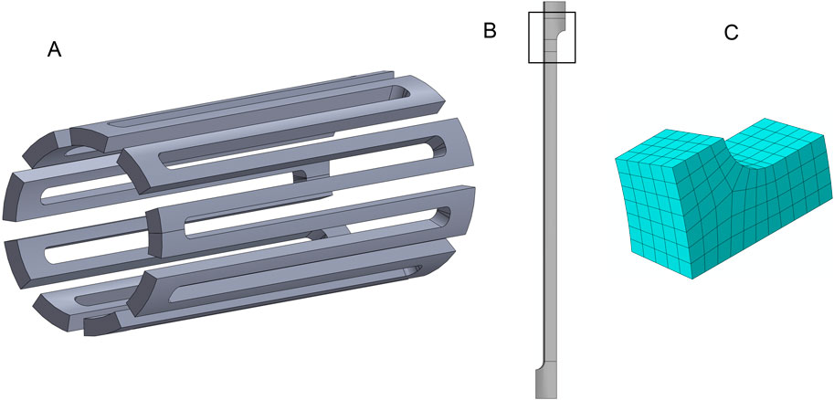
Figure 2. The laser-cut nitinol stent frame geometry. (A) A ring from a stent made of multiple repeated rings connected at the flat surfaces. (B) A single strut from the ring with the region for submodeling highlighted. (C) The submodel region is meshed with four elements across the strut width.

The computational model simulates a stent frame deployed from a catheter into an artery with a diameter 20% lower than the nominal size of the stent frame. In the simulation, the stent is expanded to a 4 mm OD from its as-cut geometry (Figure 2A), annealed, radially compressed to simulate the catheter loading process, and then released to the artery diameter. A submodel of the single strut was used to improve the efficiency of the mesh refinement process. Figure 2B highlights the geometry for the submodel with a black box.

The submodel geometry was initially meshed using hexahedral elements with an element size equal to 1/4th of the strut width, as shown in Figure 2C. The meshes for the submodel were systematically refined by reducing the element size by a factor of 2 for each refinement, resulting in models with 4, 8, 16, and 32 elements across the strut width. An entire strut model meshed with eight elements across the strut width was used to create the inputs for the strut submodels. The eight-element mesh was selected over the four-element mesh because the denser mesh was expected to more accurately represent the deformation of the strut during the expansion, compression, and release steps while incurring a reasonable computational cost.

A rigid cylinder was used to expand the full strut model to an OD of 4.00 mm, compress it to 1.50 mm, and then release it to 3.20 mm. For each deformation step, the negative Z face (Figure 3A) is fixed in the Z (axial) direction, and all the nodes on the positive Z face are constrained to have the same Z coordinate value. The nodes on the faces where the strut would connect to another strut in the circumferential direction are constrained in the theta direction. Figure 3B shows the full strut at the initial, expanded, compressed, and released diameters. After expansion, the stresses were removed from the model to simulate the annealing step in the stent manufacturing process. The displacement results from the full strut simulation are used as input to control the deformation of the submodel’s end faces. The nodes on the theta symmetry face are constrained in the theta direction (Figure 3C).

Figure 3

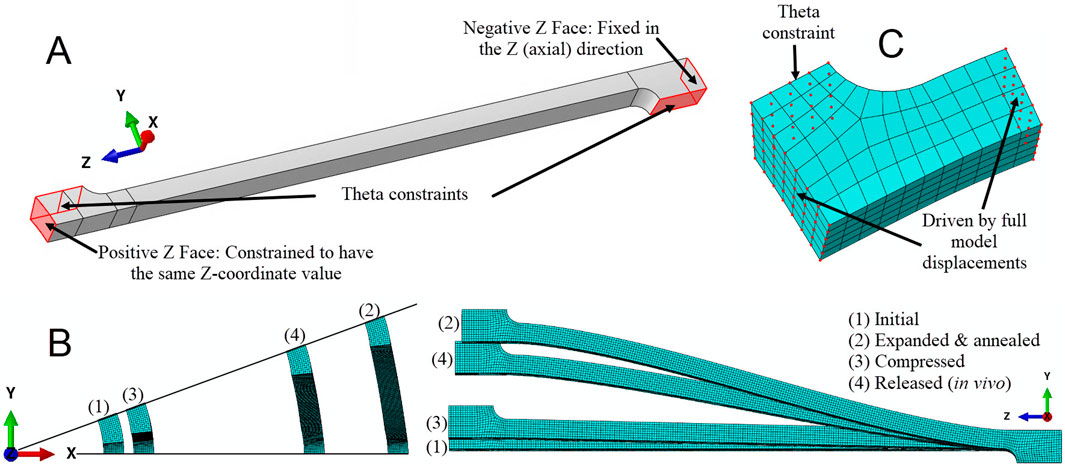
Figure 3. Deformations and constraints for the laser-cut nitinol strut. (A) Theta constraints fix nodes on the faces that connect to circumferentially adjacent struts in the circumferential direction. The nodes on the negative Z face, which connects to an adjoining ring, are fixed in the axial direction. The nodes on the positive Z face are constrained to have the same axial coordinate value. (B) Axial and side views of the strut for each step of the simulation. (C) The nodes on the face of the submodel that would connect to an adjacent strut are fixed in the circumferential direction. The nodes on the axial end faces are driven by the displacement of the corresponding nodes of the full strut model.

The stent frame example utilizes four solvers: Abaqus Explicit 2021 and Abaqus Standard 2021 (Dassault Systèmes Simulia Corp., 2020), both of which used 48 cores and C3D8R elements; LS-DYNA R12.0 (Ansys, Inc., 2020), which used 16 cores and type 2 elements with B-bar reduced integration technique; and Ansys 2023 R2 (Ansys, Inc., 2023), which used 24 cores and SOLID185 elements with reduced integration formulation. The results from each solver are anonymized, with data attributed to solvers labeled A through D. This work aims to demonstrate that the methodology applies to multiple solvers, rather than comparing the predictions of the individual solvers or analysts.

2.2 Selection of the element type for estimating the exact solution

The elements suitable for an analysis may be dictated by the features in the geometry, expected deformation modes, the material model, and the solver type. For example, a stent frame geometry from a computed tomography scan may require tetrahedral elements to approximate rounded features. After eliminating non-viable element formulations, an analyst may still have several reasonable element type choices, with accuracy and computational cost the primary factors in the final selection.

Any viable element type should yield approximately the same solution if all elements are refined to a small enough size. The difference between the output at the integration points and the exact solution for a given element size depends on the element’s order, the number of integration points, and the element’s formulation. To test this assumption, one analyst simulated three-point bending of a linear-elastic square beam to compare the convergence of peak maximum principal strain relative to element size for four different element types. This specific example was chosen because the loading is consistent with what a strut in a stent frame experiences when the device is under radial loading.

2.3 Finite element analysis of a beam under three-point bend loading

The finite element analyses of the beam used a quarter-symmetry model to represent a 0.0033-inch-per-side square cross-section with a simple linear-elastic material (8.5e6 PSI modulus, 0.35 Poisson’s ratio). Symmetry constraints are applied on the two split faces, and a displacement condition is applied along the bottom, rightmost edge of the mesh (see circled nodes in Figure 4A). The displacement initially moves the beam 0.0080 inches in the positive Y direction and then 0.0040 inches in the negative Y direction. This sequence replicates the loading conditions encountered by a stent frame when radially compressed onto a catheter delivery system and then released into a blood vessel. The peak maximum principal strains are reported for the elements in the rectangular box in Figure 4A. The strain values are reported at the integration points to avoid the extrapolation and averaging schemes used to calculate the strain at the node.

Figure 4

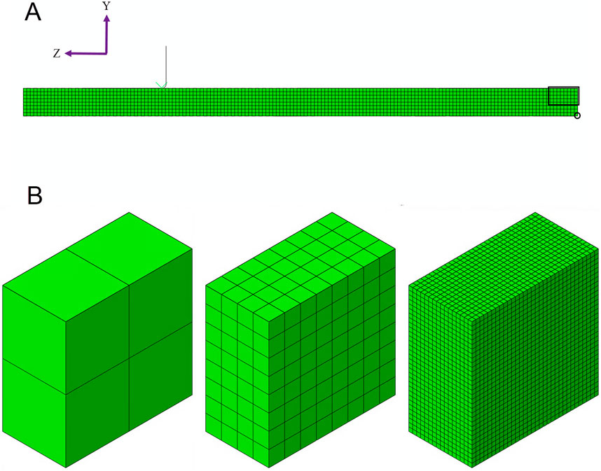
Figure 4. (A) The three-point beam bending simulation is modeled using a quarter-symmetry model, where the beam is divided in half along its length and width. The rectangular box is the region of interest for reporting the peak maximum principal strain. The nodes within the circle are used to drive the displacement of the beam. (B) Three examples of submodels are shown: 2, 8, and 32 elements through the beam’s thickness.

The number of elements through the thickness of the beam, instead of the element length, is used to characterize the mesh. Starting with an even number of initial elements through the thickness ensures that the element length through the dimension where the neutral plane intersects is consistently refined by a factor of two throughout the analysis. Meshing the entire beam with cubic elements of densities of 16 and 32 elements across the beam thickness is cost-prohibitive from a numerical perspective, even with symmetry. Therefore, submodeling was used at the end of the beam during the mesh refinement study for all mesh densities. Figure 4B illustrates the discretization of the 2-, 8-, and 32-element submodels.

Four element types for the Abaqus Standard 2021 (Dassault Systèmes Simulia Corp., 2020) solver were considered: a reduced-integration linear hexahedral element (C3D8R), a fully-integrated linear hexahedral element (C3D8), a linear hexahedral element with enhanced bending behavior (C3D8i), and a fully integrated quadratic hexahedral element (C3D20).

2.4 Options for estimating the exact solution

Richardson extrapolation estimates the converged value for a quantity of interest based on a sequence of solution outputs. For a series of three meshes with a consistent refinement factor, r, the following equation can be applied to estimate the exact solution, w_exact (ASME V&V 10.1, 2012):

$w_{exact}=w_F+\frac{w_F-w_M}{r^{p_O}-1}(2)$

where the output (w) for the mesh with the smallest element size is denoted with an F for fine, and the output for the middle element size mesh has an M for medium. The remaining undefined term is the observed order of accuracy, p_O, which is the rate of convergence of the output. The observed order of accuracy, which requires output from the fine, medium, and coarse (C) meshes, is calculated using Equation 3 (ASME V&V 10.1, 2012).

$p_O=\frac{\mathit{ln}\left(\frac{w_C-w_M}{w_M-w_F}\right)}{\mathit{ln}\left(r\right)}(3)$

This extrapolation assumes that the mesh is refined systematically and that the output data is in the asymptotic range. A systematic mesh refinement requires a uniform scaling of the element size throughout the domain. The element quality (e.g., element skewness and aspect ratio) must also remain constant or improve with refinement (Guler et al., 2022). Roy (2010) defines the asymptotic range as “the sequence of systematically refined meshes over which the discretization error reduces at the formal (theoretical) order of accuracy of the discretization scheme.” An observed order of accuracy close to the formal order of accuracy is evidence for the output data residing within the asymptotic range (ASME V&V 10.1, 2012). The formal order of accuracy of stress and strain predictions from an FEA using linear elements is 1.0 (Guler et al., 2022).

After estimating the exact solution and confirming that the output data for the three meshes fall within the asymptotic range, the analyst has to decide whether to accept the current estimate. An option for assessing the estimated exact solution is to refine the mesh once more and recalculate using the output from the three finest meshes. If the output data used to calculate the new estimate is insignificantly different from the original estimate, then it can be assumed that further refinement will not improve the estimate of the exact solution. Another option is the GCI method, which calculates the numerical uncertainty in the prediction from the fine mesh. Reducing the uncertainty, which can be calculated with 95% confidence using the Grid Convergence Index (GCI) (Roache, 1994; Roache, 2003), to a sufficiently narrow band about the predicted numerical result provides confidence that the estimated exact solution is acceptably close to the converged solution. GCI is calculated (Equation 4) using fractional change, a safety factor, F_s, the refinement factor, r, and the order of accuracy, p:

$GCI=\frac{F_s}{r^p-1}\left|\frac{w_M-w_F}{w_F}\right|(4)$

The safety factor, F_s, is usually either 1.25 or 3. Oberkampf and Roy (2010) proposed setting the value based on how close the observed order of accuracy, p_O, is to the formal order of accuracy, p_f. According to their method, if p_O is within 10% of p_f, then the safety factor is set to 1.25, and the order of accuracy in the GCI equation equals the formal order of accuracy. If p_O is not within 10% of p_f, a safety factor of 3.0 is used, and the order of accuracy in the GCI equation is equal to the minimum of p_O and p_f, but not less than 0.5.

Krysl (2022) proposed an alternative method for estimating the exact solution. His method employs a technique that uses Richardson’s extrapolation but does not require a safety factor. Instead, it requires the output from four systematically refined meshes, rather than three. This alternative method is beneficial because it does not rely on a variable safety factor to assess uncertainty. Additionally, Krysl’s method estimates the range for the true solution about the estimated exact solution rather than the finest mesh output. The method starts by defining the relative element length for each of the four meshes. The element length, h, equals the beam thickness divided by the number of elements through the thickness. The relative element length, γ, is the ratio of the mesh’s element length (h_j) to the element length of the coarsest of the four meshes (h₁) (Equation 5).

${\gamma }_j=\frac{h_j}{h_1}(5)$

There are four possible combinations of three meshes. If mesh 1 represents the coarsest mesh and mesh 4 is the finest mesh, the combinations are (1,2,3), (1,2,4), (1,3,4), and (2,3,4). The convergence rate, β, for all four possible combinations of the outputs (denoted by i) is solved for using Equation 6.

$\frac{w_{M_i}-w_{F_i}}{{{-\gamma }_{M_i}}^{{\beta }_i}+{{\gamma }_{F_i}}^{{\beta }_i}}=\frac{w_{C_i}-w_{M_i}}{{{-\gamma }_{C_i}}^{{\beta }_i}+{{\gamma }_{M_i}}^{{\beta }_i}}(6)$

The extrapolated solution, w_ext, is calculated for each combination using Equation 7.

${w_{ext}}_i={w_F}_i+C{{\gamma }_F}_i^{{\beta }_i}(7)$

where the constant C is equal to either side of Equation 6. The median extrapolated solution, $\stackrel{\sim }{w}$ _ext, of the four combinations, is then computed using Equation 8.

${\stackrel{\sim }{w}}_{ext}={median}_{i=1,2,3,4}\left(w_{{ext}_i}\right)(8)$

The estimated exact value, w_exact, is then calculated using Equation 9. It is a weighted combination of the extrapolated solution from the (2,3,4) combination, w_ext,4, and the median of all the extrapolated solutions. Krysl (2022) estimated the exact solution using a weighted average, with a 2:1 ratio of the (2,3,4) combination to the median of the four exact solutions. The weighting ratio is based on the assumption that the extrapolation from the three finest meshes provides the best estimate of the exact solution:

$w_{exact}=\left(\frac{2}{3}\right)\ast w_{{ext}_4}+\left(\frac{1}{3}\right)\ast {\stackrel{\sim }{w}}_{ext}(9)$

The uncertainty for the estimated exact solution is calculated using the median absolute deviation, as shown in Equation 10. The constant b is set to 1.4826 (Rousseeuw and Croux, 1993) under the assumption of a normal distribution.

${\stackrel{\sim }{w}}_{exact}^{MAD}=b\ast {median}_{i=1,2,3,4}\left(\left|w_{{ext}_i}-{\stackrel{\sim }{w}}_{ext}\right|\right)(10)$

Both options, using Equations 2 and 9, are explored using the C3D8R data from the three-point bend example. The estimated exact solution, the uncertainty range for the exact solution, and the resources needed for both methods are compared with the preferred method applied to the stent frame example.

2.5 Select mesh discretization options

For the stent frame example, the critical direction for the strut aligns with the strut width, as the neutral plane for strain bisects the width under the prescribed loading condition. Multiple combinations of elements through the strut width and a 1.25 aspect ratio were analyzed using a model of the full strut. This study used only reduced integration elements for consistency across all solvers, as fully integrated elements with a nitinol material model under bending can be cost-prohibitive. Each mesh is skinned in the region of interest (see boxed area of Figure 2B). For these models, the peak maximum principal strain was reported from the integration point of the skinned elements.

For the 1.25 aspect ratio meshes, the element lengths for the non-critical directions—strut thickness and axial length—were set to 25% greater than the element length in the direction of the strut width. This reduced the total number of elements without compromising the density of elements where the strain gradient is expected to be highest. Figure 5 compares the 1.0 and 1.25 aspect ratio meshes for a strut with eight elements across its width. The mesh in the black box is part of the region of interest, and the element length for the axial length direction was not modified for these elements.

Figure 5

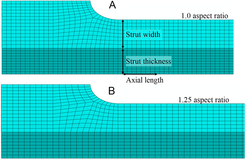
Figure 5. (A) For the mesh discretization with an aspect ratio of 1.0, the element lengths in the strut thickness and axial length directions are approximately equal to the element length in the strut width direction. The element length in the strut width direction is determined by the width of the strut and the number of elements that span the strut’s width. (B) The mesh discretization with a 1.25 aspect ratio has the same element length in the strut width direction as the 1.0 aspect ratio mesh; however, the element lengths in the strut thickness and axial length directions are approximately 25% longer than those in the strut width direction.

2.6 Calculating discretization error and computational cost

With an estimate of the exact solution, the error due to discretization, E_mag, can be calculated for each mesh. The discretization error is the absolute difference between the estimated exact solution and the output for the model (Equation 11):

$E_{{mag}_j}=\left|w_{exact}-w_j\right|(11)$

The discretization error can also be conveyed as a percentage of the estimated exact solution (Equation 12):

$E_{{pct}_j}=\frac{\left|w_{exact}-w_j\right|}{\left|w_{exact}\right|}\ast 100(12)$

Computational cost is a function of the number of cores the simulation uses and the total runtime. For the stent frame example, the computational cost was calculated for the compression and release simulation for each combination of solver and mesh. Then, for each solver, the cost for each mesh was normalized by the run time for the 1.0 aspect ratio, reduced integration linear hexahedral element model with eight elements across the strut width.

3 Results

3.1 Selection of the element type for estimating the exact solution

Figure 6 illustrates that all four element types used in the three-point bend example converge towards a peak maximum principal strain value of approximately 0.008 as the element length is refined. Therefore, a linear element with a single integration point can be as accurate as a quadratic element with over 20 integration points for this application. This suggests that a single mesh refinement study using a consistent element type may be sufficient for models similar to the bending of a beam. However, the C3D8R element mesh required four times the number of elements through the beam thickness to achieve a predicted strain value similar to that of the mesh with four C3D20 elements.

Figure 6

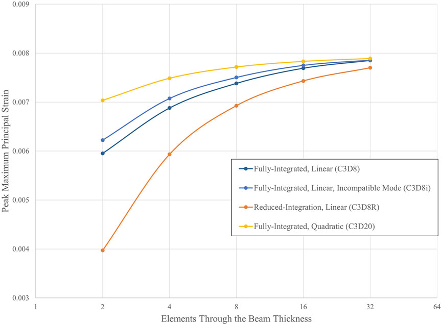
Figure 6. Convergence of peak maximum principal strain for multiple hexahedral element types. Analyses were conducted using the Abaqus/Standard solver with a linear-elastic material.

3.2 Estimating the exact solution

3.2.1 GCI method

Table 1 provides three estimates of the exact solution calculated through Richardson extrapolation from the three-point bend model. For each set of meshes, the observed order of accuracy is close to the formal order of accuracy of 1.0. Note that the estimated exact solution results align with what an observer may estimate as the converged value, as shown in Figure 6, and that using finer meshes for the calculation had a negligible impact on the result. The difference in the estimated exact solution between the finest and coarsest mesh sets is 0.000060, which is 0.75% of the result of the third set.

Table 1

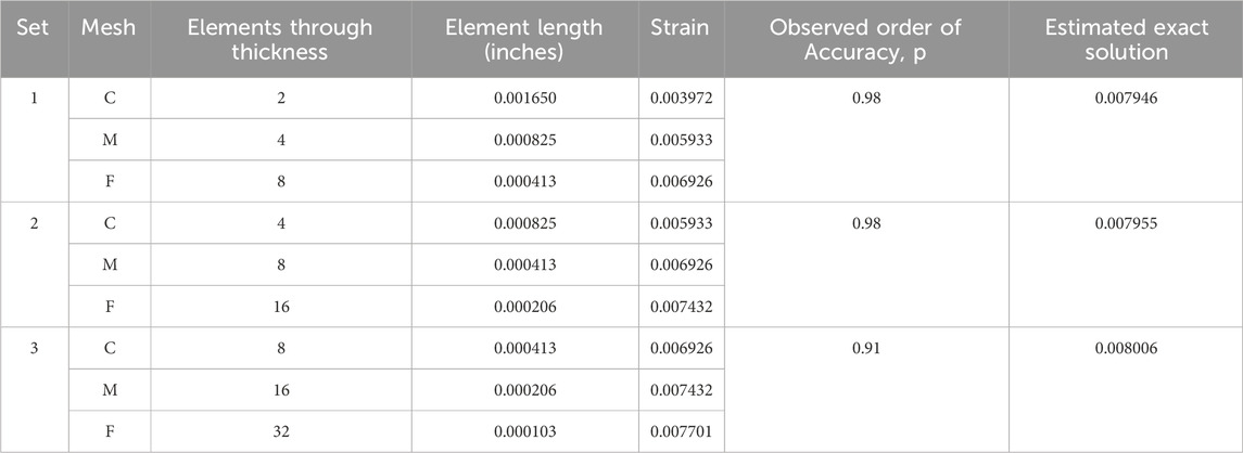
Table 1. Exact solutions estimated using Richardson extrapolation for a three-point bend model with reduced integration elements (C3D8R).

The GCI value at least halves with each successively finer set (Table 2). Correspondingly, the magnitude of the 95% confidence range for the exact solution is the smallest for the third set.

Table 2

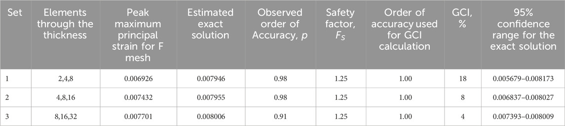
Table 2. Grid convergence index (GCI) and 95% confidence range for the exact solution for the three-point bend model with reduced integration elements (C3D8R).

3.2.2 Krysl’s method

Table 3 summarizes the results of applying Krysl’s method (Krysl, 2022) using the output from the three-point bend models. The convergence rate, β, and constant, C, values were calculated using Equation 6 and the Goal Seek function within Microsoft EXCEL 2023. The Goal Seek function, which employs the Newton method, found a value for β where the difference between the left and right sides of Equation 6 is less than or equal to 1.0E-6. The estimated exact solution, calculated using the extrapolated solutions, is 0.008000, with an uncertainty of ± 0.000040.

Table 3

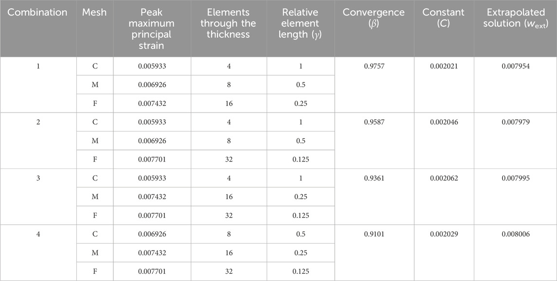
Table 3. Krysl’s Method (Krysl, 2022) for estimating the exact solution applied to the three-point bend model with reduced integration elements (C3D8R).

3.2.3 Comparison of methods

The estimated exact solutions are similar for the GCI method, which uses the three finest meshes, and Krysl’s method, which utilizes all four meshes (Table 4). Both methods calculate the 95% confidence interval for the exact solution, with the range for Krysl’s method being smaller than that of the GCI method.

Table 4

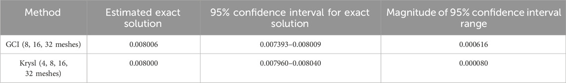
Table 4. Comparison of the estimated exact solution and 95% confidence intervals calculated using the GCI and Krysl’s method for the three-point bend model with reduced integration elements (C3D8R).

3.3 Estimate the exact solution for the laser-cut nitinol stent frame model

Table 5 lists the peak strain data, extracted from integration points, for the submodels with 4, 8, 16, and 32 elements across the strut width for all four solvers. Figure 7 illustrates the convergence of strain output for each solver. In this case, the results do not converge to approximately the same value for all the solvers. This is expected since the solvers may differ in their physics, constitutive equations, element formulations, boundary constraint methods, and parameters. For nitinol, the predicted strain from a model can be compared to the strain measured using digital image correlation (Aycock et al., 2021) on a representative sample under a bending load to assess the accuracy of the solver and material model in predicting strain. The converged solutions for each solver do not need to match to fulfill the purpose of this exercise, which is to demonstrate that the method proposed in this paper is agnostic to the solver used. Table 6 provides the results of applying Krysl’s method to find the estimated exact solution for each solver.

Table 5

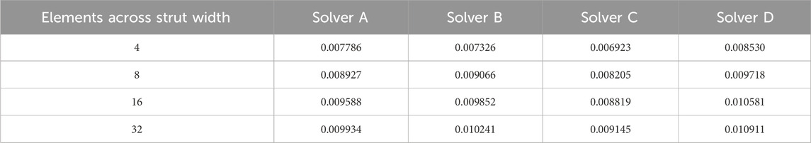
Table 5. Peak strain output data for the strut submodel.

Figure 7

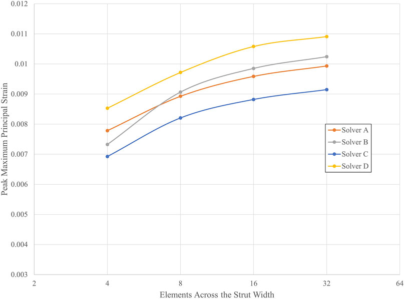
Figure 7. Convergence of peak maximum principal strain for four different FEA solvers.

Table 6

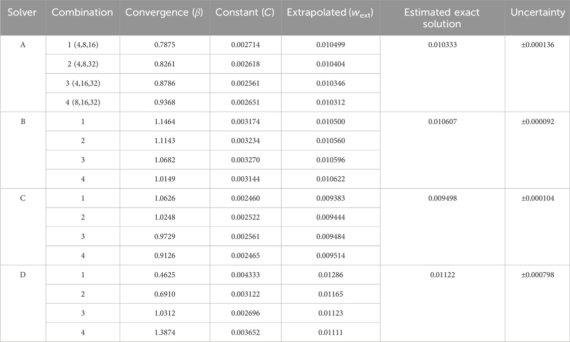
Table 6. Krysl’s method for estimating the exact solution applied to the strut model.

3.4 Select mesh discretization options for the laser-cut nitinol stent frame model

Full-strut meshes with an aspect ratio of 1.0, featuring 6 and 8 elements across the strut width, and 1.25 aspect ratio meshes with 8 and 10 elements across the strut width were simulated.

3.5 Calculate discretization error and computational cost for the discretization options

For each mesh discretization option, the computational cost and discretization error of all four solvers are summarized in Table 7. For each solver, the computational cost is normalized to the mesh with a 1.0 aspect ratio and eight elements across the strut width. As expected, the mesh with six elements across the strut width had a higher discretization error and lower computational cost than the 1.0 aspect ratio eight-element mesh. The impact of increasing the aspect ratio to 1.25 for the eight elements across the strut width models is not as clear, as three of the four solvers experienced a decrease in computational cost, accompanied by an increase in discretization error. In contrast, the fourth solver had an unchanged computational cost and slightly lower discretization error. Increasing the number of elements across the strut width to 10 while maintaining the 1.25 aspect ratio yielded mixed results. Three of the four solvers decreased the discretization error relative to the 1.0 aspect ratio eight-element mesh. Two of those three also had a relatively higher computational cost. The fourth solver, whose discretization error increased, had a lower computational cost.

Table 7

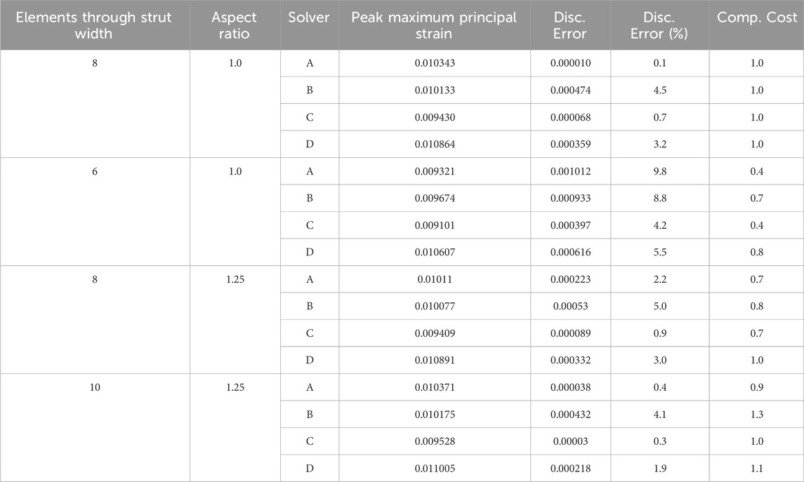
Table 7. Discretization error calculations for mesh discretization options.

4 Discussion

We explored methods for selecting the mesh discretization for a computational model of an implantable stent frame. The selection depends on the discretization error for each mesh and the computational cost. Discretization error was calculated by estimating the exact solution of the peak maximum principal strain. In our example, we simplified the stent frame to a single strut and replicated the strut undergoing shape setting, catheter loading, and deployment into a vessel. Submodeling of the region of interest reduced the resources needed for the mesh refinement study.

A mesh refinement study is necessary to estimate the exact solution. The three-point bend example showed that multiple hexahedral element types yield approximately the same solution if reporting strain at the integration point. This implies that simulations with loading modes consistent with beam bending, such as those encountered during radial loading of a stent, can utilize any hexahedral element for the mesh refinement study that is suitable for the deformation (bending) and material model. Two methods were proposed for estimating the exact solution of the peak maximum principal strain. Both methods calculate the 95% confidence interval for the exact solution. Although Krysl’s method requires four meshes, which is one more than is needed for the GCI method, we preferred it because it sets the confidence interval around the estimated exact solution rather than the prediction from the finest mesh used for extrapolation. Additionally, its confidence interval can be smaller, as shown in the three-point bend example. For both methods, the confidence interval size can inform whether the analyst can find the estimated exact solution credible or if they need to refine the mesh further and re-estimate the exact solution.

The methodology proposed in this paper improves on using fractional change to select a mesh discretization because it calculates the error in the prediction due to the geometry’s discretization and estimates the band where the exact solution is located with a 95% confidence. Fractional change can only indicate that the reduction in discretization error is decreasing. Coupled with GCI, a confidence interval for the exact solution about the finest mesh’s predicted value can be calculated. While this information is valuable, it does not provide an estimate of the exact solution.

Whether using discretization error or fractional change to quantify the impact of discretization on the numerical prediction, justifying that a mesh discretization is appropriate for the model’s COU is challenging. The COU informs the risk associated with using simulation results to make a decision that impacts patient safety and/or business interests (ASME V&V 40, 2018). Model users will prefer highly accurate predictions, especially for a COU with an elevated risk. A threshold for the maximum uncertainty in the model’s prediction can be set to determine a model’s credibility for making a decision or answering a question. Of course, the numerical uncertainty from discretization is just one aspect of the overall uncertainty, which also includes contributions from the uncertainty in the values of the model inputs (e.g., elastic modulus, dimensions) and error from model form simplifications. The authors recommend against setting a discretization error acceptance threshold, as the contribution of numerical uncertainty to the overall accuracy of a model’s output cannot be determined when conducting the mesh refinement study. Instead, we recommend selecting the mesh discretization based on the discretization error, computational cost, and knowledge of the risk associated with using the model to inform the decision. A review of the total uncertainty in the simulation output, or a poor match with validation data, may suggest the need for further mesh refinement.

The process for selecting a mesh discretization is inherently subjective. Two analysts could reasonably choose different options after arriving at the same risk assessment. Other factors, such as the projected number of simulations, license pool, and server availability, may influence the decision. Table 8 lists three realistic COUs for an implantable stent frame and their associated model risk. A mesh from Table 7 was selected for each COU, and the rationale for the selection is detailed in the table. The computational cost and discretization error for each mesh are from Solver B.

Table 8

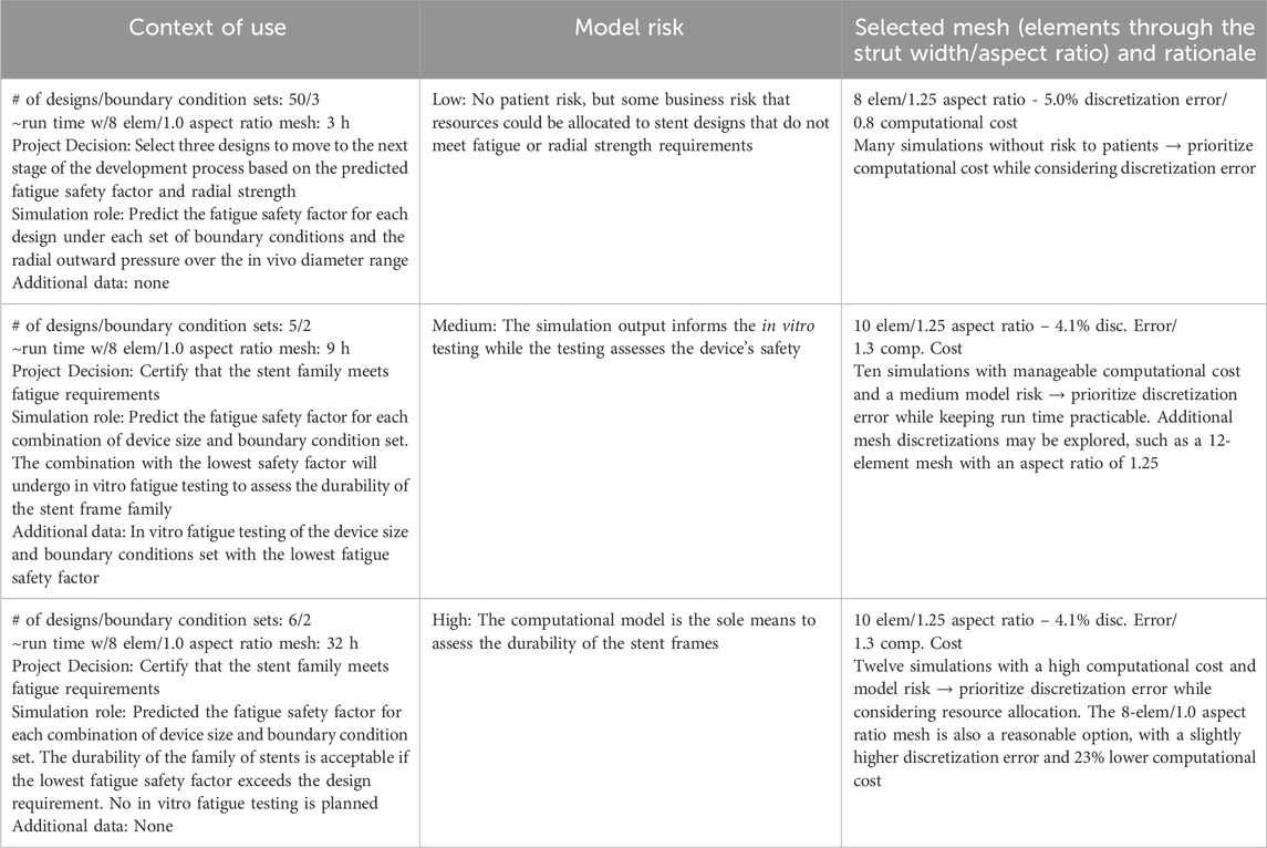
Table 8. Mesh selection based on the model’s context of use (COU).

The first COU in Table 8 does not carry a patient-related risk, but an incorrect decision could affect the project timeline. The large number of simulations and low risk led to a preference for mesh discretizations with lower computational costs. Consequently, the mesh with a 1.25 aspect ratio and eight elements across the strut width was selected. The more computationally efficient mesh with six elements across the strut width is a reasonable alternative. In our opinion, the difference in discretization error between the two, 8.8% for the six-element and 5.0% for the eight-element mesh, outweighed the small gain in computational cost, 0.7 versus 0.8. The third COU carries a high model risk with twelve simulations; each expected to take over 40 h to complete with the selected mesh discretization. While the high computational cost could serve as a motivator to use a more efficient mesh, the COU placed a significant weight on the model’s output, prompting the analyst to prioritize a low discretization error option. An additional mesh discretization, with greater than 10 elements across the strut width, could also be considered. There is no single correct answer; instead, a decision is informed by model risk, discretization error, and computational cost.

The stent example considered which mesh discretization to select based on the model risk and resource requirements for three contexts of use (Table 8), each with a different model risk. In each case, the impact of an incorrect decision, the simulation output’s influence on the decision, the combined computational cost of all the analyses, and the discretization error of the mesh options influenced the final determination of an appropriate mesh. The rationale listed for each example is provided to illustrate a logical thought process for the selection of the computational model’s mesh discretization. Experienced analysts may use similar logic and still choose a different discretization than what was presented as the best choice in the table. Though the final selection of the discretization is subjective, the outlined methodology enables an informed and defensible selection based on risk, discretization error, and computational cost.

Data availability statement

The datasets presented in this study can be found in online repositories. The names of the repository/repositories and accession number(s) can be found here: osf.io/zyust Mesh Refinement Study 2024.

Author contributions

BL: Conceptualization, Data curation, Investigation, Methodology, Project administration, Writing – original draft, Writing – review and editing. SK: Conceptualization, Data curation, Investigation, Methodology, Writing – original draft, Writing – review and editing. MH: Methodology, Resources, Writing – review and editing. CB: Conceptualization, Methodology, Writing – review and editing. SK: Data curation, Writing – review and editing. NR: Conceptualization, Methodology, Writing – review and editing.

Funding

The author(s) declare that no financial support was received for the research and/or publication of this article.

Acknowledgments

Mark Palmer, formerly with Medtronic and currently with ANSYS, and Joel Dugdale, an Associate with Gore Medical, contributed to the development of the method.

Conflict of interest

Author BL was employed by W. L. Gore and Associates, Inc. Author SK was employed by Medtronic, PLC. Author MH was employed by Ansys, Inc. Author CB was employed by Becton, Dickinson and Company. Author SK was employed by Ansys Software Private Limited. Author NR was employed by Nuno Rebelo Associates, LLC.

Generative AI statement

The author(s) declare that no Generative AI was used in the creation of this manuscript.

Publisher’s note

All claims expressed in this article are solely those of the authors and do not necessarily represent those of their affiliated organizations, or those of the publisher, the editors and the reviewers. Any product that may be evaluated in this article, or claim that may be made by its manufacturer, is not guaranteed or endorsed by the publisher.

References

ASME V&V 10.1 (2012). An illustration of the concepts of verification and validation in computational solid mechanics. New York, NY: The American Society of Mechanical Engineers.

Google Scholar

ASME V&V 40 (2018). Assessing credibility of computational modeling through verification and validation: application to medical devices. New York, NY: The American Society of Mechanical Engineers.

Google Scholar

ASTM F2996 (2020). Standard practice for finite element analysis (FEA) of non-modular metallic orthopaedic hip femoral stems. West Conshohocken, Pennsylvania: ASTM International.

Google Scholar

ASTM F3334 (2019). Standard practice for finite element analysis (FEA) of metallic orthopaedic total knee tibial components. West Conshohocken, Pennsylvania: ASTM International.

Google Scholar

Aycock, K. I., Weaver, J. D., Paranjape, H. M., Senthilnathan, K., Bonsignore, C., and Craven, B. A. (2021). Full-field microscale strain measurements of a nitinol medical device using digital image correlation. J. Mech. Behav. Biomed. Mater. 114 (2021), 104221. doi:10.1016/j.jmbbm.2020.104221

PubMed Abstract | CrossRef Full Text | Google Scholar

Guler, G., Aycock, K., and Rebelo, N. (2022) Two calculation verification metrics used in the medical device industry: revisiting the limitations of fractional change. J. Verif. Valid. Uncert. 7(3): 031004. doi:10.1115/1.4055506

CrossRef Full Text | Google Scholar

Isayama, H., Mukai, T., Itoi, T., Maetani, I., Nakai, Y., Kawakami, H., et al. (2012). Comparison of partially covered nitinol stents with partially covered stainless stents as a historical control in a multicenter study of distal malignant biliary obstruction: the WATCH study. Gastrointest. Endosc. 76 (1), 84–92. doi:10.1016/j.gie.2012.02.039

PubMed Abstract | CrossRef Full Text | Google Scholar

Karanasiou, G. S., Tachos, N. S., Sakellarios, A., Michalis, L. K., Conway, C., Edelman, E. R., et al. (2017). In silico assessment of the effects of material on stent deployment. Proc. IEEE Int. Symp. Bioinformatics. Bioeng. 2017, 462–467. doi:10.1109/BIBE.2017.00-11

PubMed Abstract | CrossRef Full Text | Google Scholar

Krysl, P. (2022). Confidence intervals for Richardson extrapolation in solid mechanics. J. Verification, Validation Uncertain. Quantification 7 (3), 031005. doi:10.1115/1.4055728

CrossRef Full Text | Google Scholar

Lurie, B. A. (2024). Mesh refinement study 2024. New York, NY: OSF. Available online at: https://osf.io/zyust/.

Google Scholar

Oberkampf, W. L., and Roy, C. J. (2010). Verification and validation in scientific computing. New York, NY: Cambridge University Press.

Google Scholar

Roache, P. J. (1994). Perspective: a method for uniform reporting of Grid refinement studies. J. Fluids Eng. 116 (3), 405–413. doi:10.1115/1.2910291

CrossRef Full Text | Google Scholar

Roache, P. J. (2003). Error bars for CFD. in: 41st Aerospace Sciences Meeting and Exhibit; 2003 January 06–09; Reno, Nevada: Aerospace Research Central.

Google Scholar

Rousseeuw, P. J., and Croux, C. (1993). Alternatives to the median absolute deviation. J. Am. Stat. Assoc. 88 (424), 1273–1283. doi:10.2307/2291267

CrossRef Full Text | Google Scholar

Roy, C. J. (2010). Review of discretization error estimators in scientific computing. AIAA Paper No. 2010-126. (Blacksburg, VA).

Google Scholar

Salamanca-Bustos, J. J., Gomez-Gomez, E., Campos-Hernández, J. p., Carrasco-Valiente, J., Ruiz-García, J., Márquez-López, F. j., et al. (2018). Initial experience in the use of novel auto-expandable metal ureteral stent in the treatment of ureter stenosis in kidney transplanted patients. Transplant. Proc. 50 (Issue 2), 587–590. doi:10.1016/j.transproceed.2017.09.048

PubMed Abstract | CrossRef Full Text | Google Scholar

Sinha, S. (2018). Modeling stents. SIMULIA Best Practices. RI, United States: Providence.

Google Scholar

Walser, E. M. (2005). Stent placement for tracheobronchial disease. Eur. J. Radiology 55 (3), 321–330. doi:10.1016/j.ejrad.2005.03.005

PubMed Abstract | CrossRef Full Text | Google Scholar