Improving aerial target detection for 3D radar based on a two-stage CFAR method with adaptive clutter distribution estimation

This study deals with the problem of enhancing aerial target detection for 3D radar. A novel approach which incorporates both signal and data processing is introduced. In order to increase the target’s SNR (signal-to-noise ratio), two consecutive transmit beams are used; for each, three beams are received simultaneously. All received beams are then processed. A two-stage constant false alarm rate (CFAR) algorithm is proposed for improving target detection. At the first-stage CFAR, the global CA-CFAR is applied to identify all possible target candidates (plots). Then, unsupervised machine learning is used to separate interference regions. For each interference region, the truncated probability density function of interference is estimated, and then a local CFAR (second-stage CFAR) is applied to reduce false plots while retaining target plots. The proposed approach is an extension of that given in recent publications. Tests on a 3D surveillance radar show the effectiveness of the proposed approach on aerial target detection in comparison with previous methods.

1 Introduction

The major role of a radar system is target detection by transmitting signals and processing the reflected signals from targets. A constant false alarm rate (CFAR) algorithm is used to decide the presence or absence of a target in a cell under test (CUT). One of the most popular CFAR algorithms is cell-averaging CFAR (CA-CFAR). CA-CFAR works well for target detection in the case of target isolation (i.e., targets are separated by at least the reference window size) and a homogeneous Gaussian environment (i.e., samples in reference cells are independent and identically distributed, and the distribution is Gaussian, like the distribution of interference in CUT) (Richard, 2005). However, in real-world scenarios, the environment is often complex (non-homogeneous) due to clutter (such as echo from surfaces, trees, meteorology, and terrain) and target masking (i.e., targets in reference cells reflect higher powers than the target in CUT). This leads to an increase in the false alarm rate and degrades the performance of CA-CFAR.

To mitigate the masking effect, smallest-of cell-averaging CFAR (SOCA-CFAR) and greatest-of cell-averaging CFAR (GOCA-CFAR) have been investigated (Hansen, 1973; Weiss, 1982). Unlike CA-CFAR, which evaluates the threshold using all reference cells, GOCA-CFAR and SOCA-CFAR only estimate the threshold using half the reference cells. They therefore need to use more reference cells than CA-CFAR.

Ordered-statistic CFAR (OS-CFAR) (Rohling, 1983) is another approach to improve classical CA-CFAR against the target masking problem. The data (reflected signal) from reference cells are arranged in an ascending sequence. Then, the $k$-element of the sequence is selected as the noise level. Blake (1988) has shown that the losses of OS-CFAR are lower than those of CA-CFAR.

Subsequent studies have extended CFAR in various directions, such as CFAR with different clutter distributions, with additional statistical tests, or with machine learning to recognize the homogeneity of the environment in reference cells. Among a larger number of works, we review some.

For CFAR with different clutter distributions, Rifkin (1994) and Baadeche and Soltani (2015) are relevant with CFAR thresholding in Weibull clutter, and Xu et al. (2015) and Zhou et al. (2018) refer to CFAR with K and gamma distributions, respectively.

For using CFAR with additional statistical tests, Finn (1986) worked with CFAR under the assumption that data from the CFAR window (including CUT) span into two different statistical regions. Smith and Varshney (2000) investigated the combination of CA-CFAR, GOCA-CFAR, and SOCA-CFAR based on second-order statistics (variability index) and the ratio of mean values of the leading and lagging reference windows. Sarma and Tufts (2001) investigated non-parametric CFAR, introducing a threshold setting algorithm without knowledge of the distribution of interference. Norouzi et al. (2007) studied detection in non-coherent radar in the case of Weibull and log-normal clutter based on goodness-of-fit tests (Kolmogorov–Smirnov, Cramer–von Mises, and Anderson–Darling tests). Zhou et al. (2017) proposed a novel CFAR combining the advantages of CA-, GOCA-, and OS-CFAR using an iterative process by sorting and amplitude-weighted averaging to estimate background level and detection in gamma distribution clutter. Mehanaoui et al. (2019) detected non-Gaussian background using the Pietra index as a measure of statistical heterogeneity instead of the variability index. Other studies in this direction are Tien et al. (2018), Zhou et al. (2019), Subramanyan et al. (2019), Lv et al. (2024), and Coluccia et al. (2024) and the references therein.

Machine learning and deep learning approaches have been intensively investigated in recent years for improving radar detection in non-homogeneous environments. Various machine learning techniques, from simple models such as support vector machines and neural networks to more complex models such as recurrent neural networks, convolutional neural networks, and YOLO, have been studied. For more details, we refer readers to Wang et al. (2017), Lu et al. (2018), Zhang et al. (2013), Perd´ock et al. (2024), and Jiang et al. (2022).

In almost all the literature mentioned above, CFAR is studied in combination with signal processing algorithms such as moving target indicator (MTI) and moving target detection (MTD) (Richard, 2005; Skolnik, 2008; Barton, 2013; Budge and German, 2015) and with the pre-defined interference distribution (for example, Gaussian distribution for noise in the entire space region and the Weibull distribution for ground clutter in the near-radar region). MTI and MTD increase the signal-to-noise ratio and hence improve the probability of detection while reducing false alarms.

However, from a practical point of view, the interference is unknown in both the type of distribution and where it may appear. It may change from region to region and scan to scan. Therefore, the use of the classical signal processing methods (MTI, MTD, and CFAR) with the same pre-defined interference distribution is not suitable. In fact, the use of MTI will increase the noise floor level in non-clutter regions (Figure 1). Moreover, the probabilities of detection $(P_d)$ and of a false alarm $(P_{fa})$ are related (Richard, 2005). Thus, in the case of complex interference environments, the choice of an interference level to maintain a required probability of detection may lead to an increased false alarm rate (Figure 2).

Figure 1

Figure 1. Signal noise floor rises as a result of MTI (red line) compared to its absence (black line).

Figure 2

Figure 2. False alarms (in yellow circles) on a radar screen due to non-homogeneous environments.

In this study, we extend the results of Tien et al. (2018) and Li et al. (2025) to propose a new approach for improving aerial target detection. The suggested method focuses on a two-stage CFAR process comprising a global CFAR in the first stage and a local CFAR based on interference distribution estimation in the second stage to improve target detection in non-homogeneous environments. This study is organized as follows: Section 2, we give a detailed statement of the problem. The proposed approach is presented in Section 3. The test results and comparison are given in Section 4. Section 5 contains the conclusion and future work.

2 Statement of the problem

In radar, detecting a target is equivalent to deciding whether “target absent” (null hypothesis, $H_0$) or “target present” (alternative hypothesis, $H_1$) is valid in the CUT (cell under test) based on measured data. Let $\mathbf{y}$ be the measured data from CUT and $p(\mathbf{y}|H_0)$ and $p(\mathbf{y}|H_1)$ be the probability density functions (PDFs) of $\mathbf{y}$ given that a target was not present (respectively, a target was present) in CUT. The probabilities of detection and of false alarms are thus evaluated (Richard, 2005; Skolnik, 2008; Barton, 2013; Budge and German, 2015):

$P_d={\int }_{\mathrm{\Omega }}p\left(\mathbf{y}|H_1\right)d\mathbf{y},(1)$

$P_{fa}={\int }_{\mathrm{\Omega }}p\left(\mathbf{y}|H_0\right)d\mathbf{y},(2)$

where $\mathrm{\Omega }$ denotes the set of $\mathbf{y}$ for which hypothesis $H_1$ will be chosen.

The Neyman–Pearson decision rule (or likelihood ratio test) is as follows:

$\frac{p\left(\mathbf{y}|H_1\right)}{p\left(\mathbf{y}|H_0\right)}{\gtrless }_{H_0}^{H_1}\lambda .(3)$

To use Equation 3, the explicit forms of $p(\mathbf{y}|H_1)$ and $p(\mathbf{y}|H_0)$, defined in Equation 1, 2, are required. Then, the threshold $\lambda$ will be estimated from $P_{fa}$.

In order to determine the pdfs $p(\mathbf{y}|H_1)$ and $p(\mathbf{y}|H_0)$, the pre-defined model of measured data $\mathbf{y}$ is given. Usually, the model of $\mathbf{y}$ used in a radar system is of the form (Richard, 2005; Skolnik, 2008; Barton, 2013; Budge and German, 2015):

$H_0:\mathbf{y}=\mathbf{n},(4)$

$H_1:\mathbf{y}=\mathbf{s}+\mathbf{n},(5)$

where $\mathbf{s}$ and $\mathbf{n}$ denote the reflected signal from CUT and system noise (Gaussian noise), respectively. Another model is added with a clutter component $\mathbf{c}$ into the right-hand side of Equations 4, 5:

$H_0:\mathbf{y}=\mathbf{n}+\mathbf{c},(6)$

$H_1:\mathbf{y}=\mathbf{s}+\mathbf{n}+\mathbf{c},(7)$

where clutter $\mathbf{c}$ follows the predefined distribution such as Weibull, K, or gamma.

Assuming that interference (noise, clutter) in the adjacent range cells has the same PDFs and characteristics as that in the CUT, we propose a general model of Equations 6, 7 for target detection:

$H_0:\mathbf{y}=\mathbf{i},(8)$

$H_1:\mathbf{y}=\mathbf{s}+\mathbf{i},(9)$

where interference $\mathbf{i}(t,x)$ at time $t$ and position $x$ has the representation

$\mathbf{i}\left(t,x\right)={\displaystyle \sum _{k=1}^m}\chi \left(x,A_k\right)p^{\left(k\right)}\left(t,x\right).(10)$

Here, $A_k$ is the disjoint region (i.e., $A_k\cap A_{k^{\prime }}=\varnothing$ for $k\ne k^{\prime }$) at which the PDFs of interference are $p^{(k)}(t,x)$, and

$\begin{array}{ll}\hfill \bigcup _{k=1}^m{A}_k& =\text{all\hspace{0.17em}the\hspace{0.17em}surveillance\hspace{0.17em}space},\hfill \\ \hfill \chi \left(x,A_k\right)& =1,\text{if}x\in A_k,\hfill \end{array}(11)$

$\chi \left(x,A_k\right)=0,\text{otherwise.}(12)$

The probability density function $p^{(k)}(t,x)$ might be the sum of different PDFs of interference that occur in the CUT:

$p^{\left(k\right)}\left(t,x\right)={\displaystyle \sum _{j=1}^{n\left(k\right)}}{\alpha }_j\left(k\right)p^{\left(k_j\right)}\left(t,x\right),{\alpha }_j\left(k\right)\in \mathbb{R}.(13)$

Models Equations 8-13 mean that the reflected signal from a position $x$ at time $t$ could be the sum of signals reflected from targets and from various types of interference with different distributions $p^{(k_j)}$ and weights ${\alpha }_j(k)$. Therefore, the CFAR with the predefined interference distribution mentioned in Section 1 degrades its performance in this situation.

In the next section, we propose a new approach to solve the detection problem Equations 8-13. The main ideas of the proposed approach are:

a. multiple beams processing for maximizing SNR;

b. using CA-CFAR (first-stage CFAR) with a global $P_{fa}$ to determine possible target candidates;

c. application of unsupervised machine learning to separate interference regions $A_k$ from all possible target candidates;

d. interference distribution estimation for each region $A_k$;

e. false candidate reduction using second-stage CFAR with a local $p_{fa}$.

3 Proposed approach

The diagram of the proposed approach is given in Figure 3. Two consecutive beams are formed in the DSP-B (digital signal processing on board) block and up-converted to operating frequency. Then, the beams are radiated into space via TRMs (transmit/receive modules) and antennas. The received signals from TRMs are passed through TRD (transmit/receive digitization) blocks in which the signals are digitized, down-converted, and then passed to the DSP-B block for digital beamforming. For each transmit beam, three beams are received in DSP-B (Subsection 3.1). These are then processed in DSP-C (digital signal processing on computer) and DP-C (data processing on computer) blocks (Subsection 3.2).

Figure 3

Figure 3. Diagram of the proposed approach.

3.1 DSP-B

The radar system transmits two consecutive beams separated by different elevation angles, with the maximum angle-distance between them being half of the elevation beamwidth. For each transmitted beam, two sets of beams (the sum, and elevation difference beams) are received in Equation 14 below:

$b_s^{\left(i\right)}\left(t\right)={\displaystyle \sum _{n=1}^N}{w}_s^{\left(i\right)}\left(n\right)r_n\left(t\right),b_{{\mathrm{\Delta }}_E}^{\left(i\right)}\left(t\right)={\displaystyle \sum _{n=1}^N}{w}_{{\mathrm{\Delta }}_E}^{\left(i\right)}\left(n\right)r_n\left(t\right),i=\mathrm{1,2,3},(14)$

where ${\{r_n(t)\}}_{n=1}^N$, ${\{w_s^{(i)}(n)\}}_{n=1}^N$, ${\{w_{{\mathrm{\Delta }}_E}^{(i)}(n)\}}_{n=1}^N$ are the digital sub-array data and beamforming weights, respectively. The maximum angle-distance between simultaneously received beams (corresponding to each transmitted beam) is equal to one-fourth of the elevation beamwidth (Figure 4).

Figure 4

Figure 4. Example of two transmitted beams (up) and six received beams (bottom) at the output of digital beamforming in DSP-B.

3.2 DSP-C and DP-C

Received beams are then processed in DSP-C, including PC (pulse compression), MTI/MTD (for pulse integration), and first-stage CFAR (using CA-CFAR with a given global $P_{fa}$). The beam with maximum detection performance (Yu, 2009, Scheme 3) is selected in “beam selection” (Figure 3).

In the case of non-homogeneous environments, false alarms occur after the first-stage CFAR. For air-defense radars, most popular false alarms are due to reflected echoes of surface or meteorology and have some typical characteristics, such as higher density (the density of plots in clutter regions is higher than in other non-clutter regions) and stability (the false plots due to clutter remain in the clutter regions are longer than in non-clutter regions). Based on these characteristics, density-based clustering based on the hierarchical density estimates (HDBSCAN) algorithm is used for “interference clustering” in DP-C. The main steps of the HDBSCAN algorithm are given in Campello et al. (2013). The output of the interference clustering is the set of interference regions $A_k$, $k=1,\dots ,m$, $m\ge 1$. For each region $A_k$, let $N_k$ be the number of plots in $A_k$ and ${\left\{y_i^{(k)}\right\}}_{i=1}^{N_k}$ be the set of plot powers in $A_k$. The interference PDF in $A_k$ is approximated using polynomials in Algorithm 2 (Table 2). Here, we use the polynomial approximation in order to simplify execution while keeping a satisfactory result. The main steps processed in DSP-C and DP-C are given in Algorithm 1 (Table 1). We note that in formula 15, the function $F_k$ is the cumulative distribution function corresponding to the interference PDF $p^{(k)}$, which by virtue of which Algorithm 2 (Table 2) is a polynomial. Therefore, $F_k$ is a continuous and strictly increasing function. This implies that it is invertible, with formula 15 being consistent (Table 1).

Table 1

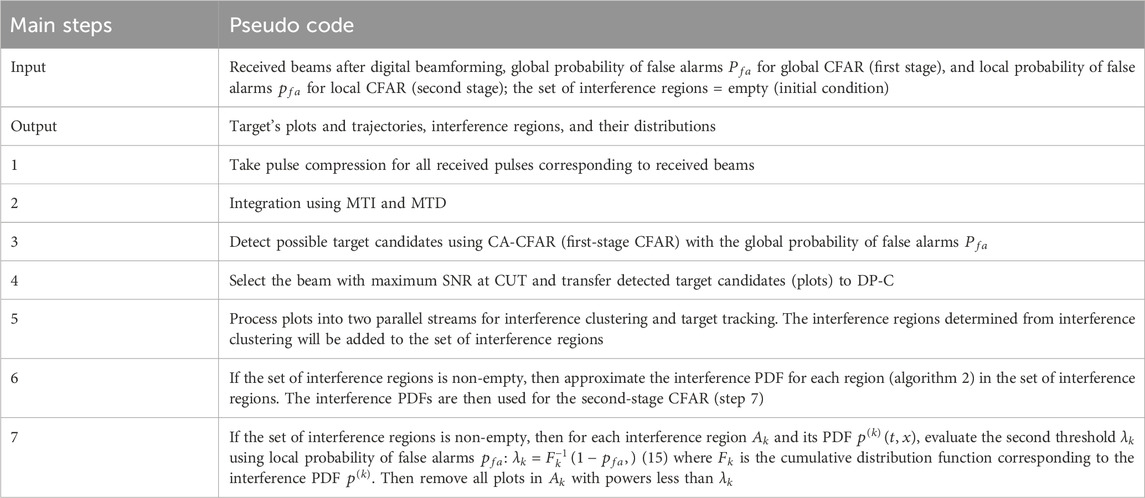
Table 1. Algorithm 1 (processing in DSP-C and DP-C).

Table 2

Table 2. Algorithm 2 (interference probability density function estimation).

4 Test results and comparison

The radar used for the test is an air-defense 3D surveillance radar (Figure 5) with system parameters given in Table 3. The value $p_{fa}$ will be used for interference regions to reduce false alarms. This value is the default false alarm rate used in Li et al,(2025). Elevation scanning is achieved by electronically adjusting the phase of signals across an antenna array, while azimuth scanning is accomplished by physically rotating the antenna. At each steering angle, two consecutive beams are transmitted and six are received (Figure 4). The angle-distance between two consecutive transmitted beams equals 1.4°, while the angle-distance between simultaneously received beams (corresponding to each transmitted beam) equals 0.5° (Figure 4). The target used for the test is a light-sport aircraft, the ATEC 321 Faeta (Figure 6), which flies at a velocity of 160 km per hour at an altitude of 1000 m. The tests were carried out on an Ubuntu system and the C++ software platform. For DSP-C and for DP-C, we use three computers with Intel Xeon Gold 6242R 3.1 GHz (20 cores, 40 threads) and 24 GB of RAM. The computational time required in DSP-C is less than 1 ms, and that in DP-C is less than 0.3 s. This approach guarantees that the online processing for the radar system since the time of one radar scan is 10 s (Table 3).

Figure 5

Figure 5. Radar used for the test.

Table 3

Table 3. Radar system parameters used for the test.

Figure 6

Figure 6. Aircraft used for the test (Source: internet).

The test showed that the interference mean powers between 13 km and 80 km with respect to the transmitted beams at 0.6° and 2.0° are approximately 33 dB and 18 dB, respectively (Figure 7). This induces an increase of the target’s SNR with an averaging value of 11 dB (Figures 8, 9) and hence improves target detection at the first-stage CFAR (Figure 10). Since the threshold of the first-stage CFAR is chosen for the case of Gaussian noise, there are false plots in interference regions due to the difference of interference PDFs from normal. Furthermore, in the radar data processing, the false plots are clustered using the HDBSCAN algorithm with parameters given in Table 4. The values of $k$ mean that the first radar scan is used for interference clustering, and then every minute (equivalently every 6 radar scans) these interference regions are checked and updated. The results of interference clustering are shown in Figure 10 (in polygons).

Figure 7

Figure 7. Interference mean powers corresponding to two transmitted beams.

Figure 8

Figure 8. At range of 70 km, target’s SNR corresponding to the beam at an elevation of 0.6 degree is 10 dB.

Figure 9

Figure 9. At range of 70 km, target’s SNR corresponding to the beam at an elevation of 2.0 degree is 18 dB.

Figure 10

Figure 10. Result of first-stage CFAR: test target (in white circle) and false alarms due to interference (in polygons).

Table 4

Table 4. Parameters for HDBSCAN algorithm used in the tests.

For each interference region, the interference PDF can be estimated using Algorithm 2. The results of probability density function approximation show (Figures 11) that the method using Bernstein’s polynomial performs better than that using probability moments. Here, for the false plot reduction in the second-stage CFAR, we use Bernstein’s approximation with $n=6$, the local probability of false alarms $p_{fa}=0.1$ for all interference regions, and the thresholds evaluated by (15) (Figure 12). The result of second-stage CFAR is given in Figure 13.

Figure 11

Figure 11. PDFs of the target (red curves) used for test and of interference (black curves) by Bernstein’s (solid lines) and moment (dashed lines) methods.

Figure 12

Figure 12. Threshold for second-stage CFAR of the interference region having the test target.

Figure 13

Figure 13. Results after second-stage CFAR. Test target is in white circle.

For comparison, note that the interference probability density function is estimated using Bernstein’s polynomial, which could be more suitable for various types of interference than the use of kernel density estimation in Budge and German (2015). Additionally, we look at the situation where other CFAR algorithms like OS, SOCA, GOCA, VI, and PI, which have thresholds listed in Supplementary Appendix 2, are applied in the first-stage CFAR, while the second-stage CFAR is not used. The following detection performance parameters are used for comparison (Sunnen et al., 1997).

a. $P_{d_c}$: probability of target detection in the interference region, which is defined by the number of target reports over the number of antenna scans in the interference region.

b. $FT{r}_c$: false target reports are defined by the average number of such reports in clutter regions per antenna scan.

c. $TD{r}_c$: track drop rate in the clutter region. $TD{r}_c=1$ where the track is dropped when the test target is moving in a clutter region; otherwise, $TD{r}_c=0$.

With the same value $P_{fa}=10^{-3}$, the coefficient $\alpha$ (Supplementary Appendix 2) for CFAR threshold calculating and detection performance is given in Table 5 and Figures 14–18. Note that the $\alpha$ value of the proposed approach given in Table 5 is of the first-stage CFAR (CA-CFAR). The threshold for second-stage CFAR is approximately −61 dBm (Figure 12). The thresholds of VI-CFAR are $K_{VI}=5.3$ and $K_{MR}=2.1$, while the thresholds of PI-CFAR are $T_{PI}=3$ and $T_{MR}=1.5$. The test results show that by using the proposed approach, we can track the target over the interference region, while with other methods the track is dropped when the target moves into the interference region. Moreover, the false track reports (per antenna scan) of the proposed approach are much fewer than others.

Table 5

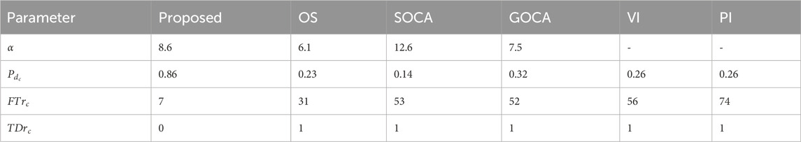
Table 5. Comparison of proposed approach with other CFAR algorithms.

Figure 14

Figure 14. Test using OS-CFAR. Test target is in white circle.

Figure 15

Figure 15. Test using SOCA-CFAR. Test target is in white circle.

Figure 16

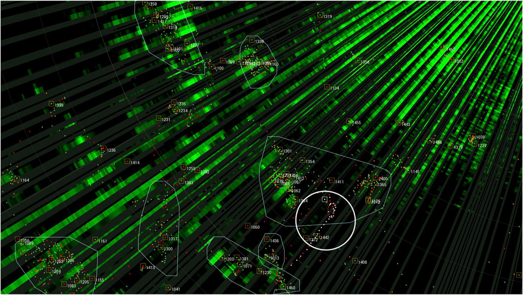
Figure 16. Test using GOCA-CFAR. Test target is in white circle.

Figure 17

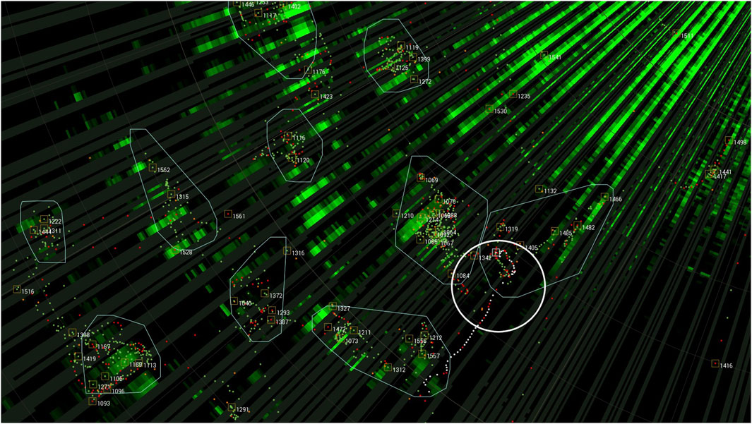
Figure 17. Test using VI-CFAR. Test target is in white circle.

Figure 18

Figure 18. Test using PI-CFAR. Test target is in white circle.

Compared with the machine learning approach (Perd´ock et al., 2024), we note that in our test, the target’s SNR is only approximately 10 dB (Figure 8), and hence the approach in Perd´ock et al. (2024) gives the value $P_{d_c}\approx 0.6$ according to $P_{fa}=0.1$ [Perd’ock et al. (2024), Figures 19, 22]. This value shows the superior performance of our proposed approach.

5 Conclusion and future work

This study presents a new approach for improving aerial target detection for 3D radars while working in non-homogeneous environments based on multiple beam processing, interference clustering, and its PDF approximation. Although the problem of PDF estimation is well-known and has been studied for more than a century, the discovery that the target’s and the interference PDFs are truncated for a radar system guarantees that the approximations are consistent—there are no other PDFs with the same approximations as Supplementary Appendix Equations A2, A14. The test and comparison show the effectiveness of the proposed approach.

In future research, instead of using the same value $p_{fa}=0.1$ for all interference regions as in this study, we will apply optimization theory to select the optimal local probability of false alarms $p_{fa}$ value for each interference region. In addition, new results in the probability distribution estimation problem will be considered for enhancing radar detection performance.

Data availability statement

The raw data supporting the conclusions of this article will be made available by the authors, without undue reservation.

Author contributions

TV: Conceptualization, Data curation, Formal Analysis, Project administration, Software, Validation, Visualization, Writing – original draft, Writing – review and editing. TC: Conceptualization, Supervision, Validation, Writing – review and editing. NV: Conceptualization, Data curation, Supervision, Validation, Writing – review and editing.

Funding

The authors declare that financial support was received for the research and/or publication of this article. The publication of this article is supported by the Viettel High Technology Industries Corporation.

Acknowledgments

Acknowledgements

The authors would like to thank the reviewers for all their careful, constructive, and insightful comments that improved the paper.

Conflict of interest

The authors declare that this study received funding from Viettel High Technology Industries Corporation. The funder had the following involvement in the study: decision to submit it, and payment for publication.

Generative AI statement

The authors declare that no Generative AI was used in the creation of this manuscript.

Any alternative text (alt text) provided alongside figures in this article has been generated by Frontiers with the support of artificial intelligence and reasonable efforts have been made to ensure accuracy, including review by the authors wherever possible. If you identify any issues, please contact us.

Publisher’s note

All claims expressed in this article are solely those of the authors and do not necessarily represent those of their affiliated organizations, or those of the publisher, the editors and the reviewers. Any product that may be evaluated in this article, or claim that may be made by its manufacturer, is not guaranteed or endorsed by the publisher.

Supplementary material

The Supplementary Material for this article can be found online at: https://www.frontiersin.org/articles/10.3389/frsip.2025.1688944/full#supplementary-material

References

Baadeche, M., and Soltani, F. (2015). Performance analysis of mean level constant false alarm rate detectors with binary integration in weibull background. IET Radar Sonar Navig. 9 (3), 233–240. doi:10.1049/iet-rsn.2014.0053

CrossRef Full Text | Google Scholar

Barton, D. (2013). Radar equations for modern radar. Boston: Artech House.

Google Scholar

Blake, S. (1988). OS-CFAR theory for multiple targets and nonuniform clutter. IEEE Trans. Aero. Electron Syst. 24 (6), 785–790. doi:10.1109/7.18645

CrossRef Full Text | Google Scholar

Budge, M., and German, S. (2015). Basic radar analysis. Boston: Artech House.

Google Scholar

Campello, R., Moulavi, D., and Sander, J. (2013). “Density-based clustering based on hierarchical density estimates,” in Advances in knowledge discovery and data mining. Editors J. Pei, V. Tseng, L. Cao, H. Motoda, and G. Xu (Berlin, Heidelberg: Springer), 169–172.

CrossRef Full Text | Google Scholar

Coluccia, A., Orlando, D., and Ricci, G. (2024). Adaptive radar detection in heterogeneous clutter plus thermal noise via the expectation-maximization algorithm. IEEE Trans. Aerosp. Electron. Syst. 60 (1), 212–225. doi:10.1109/taes.2023.3322389

CrossRef Full Text | Google Scholar

Finn, M. (1986). A CFAR design for a window spanning two clutter fields. IEEE Trans. Aero. Electron Syst. 22 (2), 155–169. doi:10.1109/taes.1986.310750

CrossRef Full Text | Google Scholar

Hansen, V. G. (1973). “Constant false alarm rate processing in search radars,” in Proceedings of the IEE international radar conference (London, UK).

Google Scholar

Jiang, W., Ren, Y., Liu, Y., and Leng, J. (2022). Artificial neural networks and deep learning techniques applied to radar target detection: a review. Electronics 11 (1), 156. doi:10.3390/electronics11010156

CrossRef Full Text | Google Scholar

Li, S., Wei, H., Mao, Y., and Fan, J. (2025). A novel two-stage superpixel CFAR method based on truncated KDE model for target detection in SAR images. Electronics 14, 1327. doi:10.3390/electronics14071327

CrossRef Full Text | Google Scholar

Lu, S., Yi, W., Liu, W., Cui, G., Kong, L., and Yang, X. (2018). Data-dependent clustering CFAR detector in heterogeneous environment. IEEE Trans. Aero. Electron Syst. 54 (1), 476–485. doi:10.1109/taes.2017.2740065

CrossRef Full Text | Google Scholar

Lv, C., Li, G., Huang, X., and Liu, D. (2024). Constant false alarm detection algorithm based on KL scattering. Int. J. RF Microw. Comp.-Aided Eng. 2024, 2218790. doi:10.1155/2024/2218790

CrossRef Full Text | Google Scholar

Mehanaoui, A., Laroussi, T., and Mezache, A. (2019). Pietra index based processor for a heterogeneous pareto background. IET Radar Sonar Navig. 13 (8), 1225–1233. doi:10.1049/iet-rsn.2018.5608

CrossRef Full Text | Google Scholar

Norouzi, Y., Gini, F., Nayebi, M., and Greco, M. (2007). Non-coherent radar CFAR detection based on goodness-of-fit tests. IET Radar Sonar Navig. 1 (2), 98–105. doi:10.1049/iet-rsn:20060032

CrossRef Full Text | Google Scholar

Perd´ock, J., Gazˇovova´, S., and Pacek, M. (2024). An improved radar clutter suppression by simple neural network. In: Adv. AI-assisted radar Sens. Appl., ed. S. Vishwakarma, K. Chetty, J. Kernec, Q. Chen, R. Adve, and S. Gurbuz (IET Radar, Sonar and Navigation, 18(2), 308–326). doi:10.1049/rsn2.12510

CrossRef Full Text | Google Scholar

Richard, M. A. (2005). Fundamentals of radar signal processing. New York: McGraw-Hill.

Google Scholar

Rifkin, R. (1994). Analysis of CFAR performance in weibull clutter. IEEE Trans. Aero. Electron Syst. 30 (2), 315–329. doi:10.1109/7.272257

CrossRef Full Text | Google Scholar

Rohling, H. (1983). Radar CFAR thresholding in clutter and multiple target situations. IEEE Trans. Aero. Electron Syst. 19 (4), 608–621. doi:10.1109/taes.1983.309350

CrossRef Full Text | Google Scholar

Sarma, A., and Tufts, D. (2001). Robust adaptive threshold for control of false alarms. IEEE Signal Proc. Lett. 8 (9), 261–263. doi:10.1109/97.948451

CrossRef Full Text | Google Scholar

Skolnik, M. (2008). Radar handbook. New York: McGraw-Hill.

Google Scholar

Smith, M., and Varshney, P. (2000). Intelligent CFAR processor based on data variability. IEEE Trans. Aero. Electron Syst. 36 (3), 837–847. doi:10.1109/7.869503

CrossRef Full Text | Google Scholar

Subramanyan, N., Kalpathi, R., and Vengadarajan, A. (2019). Robust variability index CFAR for non-homogeneous background. IET Radar Sonar Navig. 13 (10), 1775–1786. doi:10.1049/iet-rsn.2018.5435

CrossRef Full Text | Google Scholar

Sunnen, A., Escritt, P., and Philipp, W. (1997). “Radar surveillance in en-route airspace and major terminal areas,” in Eurocontrol standard document SUR.ET1.ST01.1000-STD-01-01 (Brussels, Belgium: Eurocontrol Agency).

Google Scholar

Tien, V., Hop, T., Nam, L., Thanh, T., and Loi, N. (2018). “An adaptive 2D-OS-CFAR thresholding in clutter environments: test with real data,” in Proceedings of the 2018 5th int. Conf. Sig. Proc. and integrated Netw. (SPIN2018) (Noida, India).

Google Scholar

Wang, L., Wang, D., and Hao, C. (2017). Intelligent CFAR detector based on support vector machine. IEEE Access 5, 26965–26972. doi:10.1109/access.2017.2774262

CrossRef Full Text | Google Scholar

Weiss, M. (1982). Analysis of some modified cell-averaging CFAR processors in multiple-target situations. IEEE Trans. Aero. Electron Syst. 18 (1), 102–114. doi:10.1109/taes.1982.309210

CrossRef Full Text | Google Scholar

Xu, Y., Yan, S., Ma, X., and Hou, C. (2015). Fuzzy soft detection CFAR for the K distribution data. IEEE Trans. Aero. Electron Syst. 51 (4), 3001–3013. doi:10.1109/taes.2015.140817

CrossRef Full Text | Google Scholar

Yu, K.-B. (2009). “Digital beamforming of multiple simultaneous beams for improved target search,” in Proceeding of 2009 IEEE Radar Conference, Pasadena, CA, USA, 1–5. doi:10.1109/radar.2009.4977010

CrossRef Full Text | Google Scholar

Zhang, R., Sheng, W., and Ma, X. (2013). Improved switching CFAR detector for non-homogeneous environments. Signal Process. 93 (1), 35–48. doi:10.1016/j.sigpro.2012.06.015

CrossRef Full Text | Google Scholar

Zhou, W., Xie, J., Li, G., and Du, Y. (2017). Robust CFAR detector with weighted amplitude iteration in nonhomogeneous sea clutter. IEEE Trans. Aero. Electron Syst. 53 (3), 1520–1535. doi:10.1109/taes.2017.2671798

CrossRef Full Text | Google Scholar

Zhou, W., Xie, J., Zhang, B., and Li, G. (2018). Maximum likelihood detector in Gamma-distributed sea clutter. IEEE Geosci. Remote Sens. Lett. 15 (11), 1705–1709. doi:10.1109/lgrs.2018.2859785

CrossRef Full Text | Google Scholar

Zhou, W., Xie, J., Xi, K., and Du, Y. (2019). Modified cell averaging CFAR detector based on Grubbs criterion in non-homogeneous background. IET Radar Sonar Navig. 13 (1), 104–112. doi:10.1049/iet-rsn.2018.5160

CrossRef Full Text | Google Scholar