Research on short-term line loss rate prediction method of distribution network based on RF-CNN-LSTM

Under the background of the new distribution network, the power fluctuation on the line is increasing, which leads to more uncertainties in the predicted line loss rate, thus affecting the economic benefits of the power grid. In order to reduce the prediction error of short-term line loss rate and improve its prediction accuracy, this paper studies a short-term line loss rate prediction method of distribution network based on RF-CNN-LSTM. Firstly, this paper comprehensively considers the influence of various uncertain factors on the accuracy of prediction results. Aiming at the characteristics of high-dimensional time series of line loss rate data, a random forest (RF) algorithm is proposed to analyze the importance of multiple characteristic variables affecting line loss rate. Then, this paper constructs a combined model of convolutional neural network and long short-term memory network (CNN-LSTM) to predict line loss rate. Finally, in order to verify the accuracy of the prediction results, this paper sets up a support vector machine algorithm for synchronous prediction as a comparative experiment. The experimental results show that the prediction results of the proposed prediction method are more accurate.

1 Introduction

Line loss rate is an important economic and technical index for measuring the design, operation, maintenance, and management level of a power grid system. Ensuring the stable and economic operation of the power grid and improving the efficiency of power supply are of great significance. Under the goal of “double carbon,” the energy production level is low carbon, the level of energy consumption electrification is increasing, and the power load is increasing. The line loss of a low-voltage distribution network accounts for ~40% of the whole power network loss. The large amount of distributed power access also makes line loss management more complicated. Therefore, accurately predicting the line loss rate of a distribution network for its scientific management, energy savings, and loss reduction of the distribution network is of great practical importance (Xiaoke et al., 2023; Yinbiao et al., 2021a).

With the rapid development of artificial intelligence technology, modern intelligent prediction methods are gradually replacing classical prediction methods. As a bionic computing model, neural networks can simulate human or animal nervous systems' neurons and connect to each other for information processing. The neural network can fully adaptively improve its prediction ability according to the training set of the predicted data. (Guo et al. 2023) used deep learning models such as artificial neural networks (ANNs), long-term and short-term memory neural networks (LSTMs), convolutional neural networks (CNNs), and convolutional neural network and long short-term memory networks (CNN-LSTMs) to predict the monthly average and extreme atmospheric temperature changes in Zhengzhou. (Guo et al. 2024a) also used artificial intelligence models, such as LSTMs, CNNs, and CNN-LSTMs, to simulate the climate parameters of Jinan City, China.

In the context of the new distribution network, power fluctuations on the transmission line are increasing, which will lead to more uncertainties in the predicted line loss rate, thus affecting the power grid's economic benefits (Yinbiao et al., 2021b). How intelligent algorithms can be used to optimize the existing line loss rate prediction model to improve prediction accuracy has become a current research hot spot. With the random forest (RF) algorithm proposed by Leo Breiman in 2001, power data prediction has reached a new level. Its unique feature extraction advantages are applied to various fields. In a study by (Yiwen 2022), the RF algorithm is used to sort and screen the characteristic quantities of the influencing factors of line loss rate according to the contribution rate, and then the least squares support vector machine algorithm is used to predict the confidence interval of line loss rate. In a study by (Qi et al. 2022), RF combined with IF–THEN rule output feature selection is used to test the average error. (Han et al. 2018) (Han et al. 2018) proposed a new feature selection method for the random forest algorithm. The example analysis shows that the prediction accuracy is 5% higher than that of a traditional back propagation neural network (BP), recurrent neural network (RNN), and support vector machine (SVM). (Jianhua et al. 2020) used the existing high-precision long short-term memory neural network (LSTM) to predict regional line loss, and the results showed that the predicted value was close to the actual value.

In general, we can predict the line loss rate according to the time scale. At present, predicting line loss rates mainly focuses on medium- and long-term predictions; a few studies on short-term line loss rate prediction are based on the week, day, and hour. Moreover, many factors affect high voltage line loss rates, and large fluctuations in the data will also lead to the prediction results having low accuracy. However, short-term line loss forecasting is also an indispensable part of power grid line loss rate prediction (Yingchun et al., 2020). In light of such problems, this article comprehensively considers the influence of the uncertain factors faced by the line loss rate during the prediction period on the prediction results' accuracy, combines the optimization algorithm to optimize the existing line loss rate prediction model, and constructs a model suitable for short-term line loss rate prediction. First, the influencing factors of short-term line loss rate and data preprocessing are analyzed. Secondly, this paper proposes a random forest ( RF ) algorithm to analyze the importance of multiple feature variables that affect the line loss rate. Remove the less influential feature variables and select the more important features and line loss rate data to input into the prediction model, so as to reduce the data dimension and improve the prediction efficiency and prediction accuracy. Then, a CNN-LSTM model with a better prediction effect is constructed, and an RF algorithm is used to extract important influencing variables to ensure that the line loss rate can be accurately predicted. Finally, the CNN-SVM model, which is also good at dealing with high-dimensional data, is introduced to ensure the reliability of the prediction model.

2 Data pre-processing

2.1 Theoretical line loss calculation method

Line loss, in the traditional sense, refers to the power loss generated during the power transmission process due to the presence of resistance and reactance in the transmission line, including double-winding, three-winding transformer loss, reactor element loss, and wire loss, among others. Usually, to simplify the concept and calculation, we often subtract the numerical value of the electric energy at the beginning and the end of the transmission line to obtain the line loss. In the power marketing department, line loss can also be expressed as the difference between the power supply of the power grid and the power sales of each company, and the ratio of the difference to the power supply is defined as the line loss rate. The relationship is shown in Equation 1:

$\begin{array}{ll}\text{Ratio of line loss}=\frac{\text{Electricity sales}}{\text{Power supply quantity}}\times 100\%& (1)\end{array}$

The transmission line is equipped with a meter at the beginning and end of the transmission line to record the amount of electricity. For example, the line loss of the 10-kV line in the power transmission process can be expressed as the amount of electricity measured by the first end meter minus the amount of electricity measured by the end meter. To facilitate defining this power difference in practical engineering, it is called the line loss rate, and the amount of electricity represents the difference.

In the low-voltage distribution network, due to the characteristic long lines and wide distribution and considering the irregular distribution of load along the road and the complexity of the power supply mode of the distribution network, the equivalent resistance concept is introduced. To simplify the distribution network's equivalent model, the distribution network line's resistance is equivalent to the total resistance, which is easy to calculate. The commonly used method is to place an electric energy meter at the gate. After recording the current, the resistance after the gate can be equivalent by using a quantitative relationship to obtain a resistance, R_eq, so that the total electric energy loss can be directly calculated, which is equivalent to the sum of the losses of each branch after the gate.

The distribution network line is shown in Figure 1. The equivalent resistance of each branch is R₁, R₂, R₃, ..., R_n. The current of each branch is I₁, I₂, I₃, ..., I_n. When the working time is t, the sum of the energy loss of each line of the distribution network is as shown in Equation 2:

$\begin{array}{ll}\text{Δ}A=3\times (I_1^2{R}_1+I_2^2{R}_2+I_3^2{R}_3+\cdots +I_n^2{R}_n)t\times {10}^{-3}(\text{kW}·\text{h})& (2)\end{array}$

In the actual low-voltage distribution network, accurately measuring the current is often difficult, so power consumption is often used instead of current. The relationship between the electric quantity and the current is shown in Equation 3:

$\begin{array}{ll}\frac{I_n}{I_{\text{Σ}}}=\frac{A_n}{A_{\text{Σ}}},& (3)\end{array}$

where A_n(n = 1, 2, ..., n) is the power of each branch and A_Σ is the total power of the gateway.

Figure 1

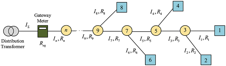
Figure 1. Distribution network circuit diagram.

Equation 2 can also be expressed as Equation 4:

$\begin{array}{l}\text{Δ}A=3I_{\text{Σ}}^2[{\left(\frac{A_1}{A_{\text{Σ}}}\right)}^2{R}_1+{\left(\frac{A_2}{A_{\text{Σ}}}\right)}^2{R}_2+{\left(\frac{A_3}{A_{\text{Σ}}}\right)}^2{R}_3+\cdots \\ +{\left(\frac{A_n}{A_{\text{Σ}}}\right)}^2{R}_n]\times t\times {10}^{-3}(\text{kW}·\text{h}).& (4)\end{array}$

The active power loss formula is shown in Equation 5:

$\begin{array}{ll}\text{Δ}P=3{\displaystyle \sum _{i=1}^n{I}_i^3}{R}_i=3I_{\text{Σ}}^3{R}_{eq},& (5)\end{array}$

where I_i represents the current flowing on line i, I_Σ represents the total current of the gateway load, and R_eq represents the equivalent resistance.

The equivalent resistance of the distribution network line is shown in Equation 6:

$\begin{array}{ll}{R}_{\text{eq}}={\left(\frac{A_1}{A_{\text{Σ}}}\right)}^2{R}_1+{\left(\frac{A_2}{A_{\text{Σ}}}\right)}^2{R}_2+{\left(\frac{A_3}{A_{\text{Σ}}}\right)}^2{R}_3+\cdots +{\left(\frac{A_n}{A_{\text{Σ}}}\right)}^2{R}_n& (6)\end{array}$

In general, the load, length, and line type of each branch are different. The calculation method for equivalent resistance is shown in Equation 7:

$\begin{array}{ll}{R}_{\text{eq}}=\frac{{\displaystyle \sum _{j=1}^n}{A}_{j·\text{Σ}}^2{R}_j}{{\left({\displaystyle \sum _{j=1}^m}{A}_i\right)}^2}& (7)\end{array}$

$\begin{array}{ll}{R}_j=r_j\times L_j& (8)\end{array}$

where R_j is the resistance of each wire, r_j is the resistance value of unit length conductor, and L_j is to calculate the length of branch wire.

2.2 Data pre-processing

To ensure the accuracy and rationality of the line loss rate data, cleaning the line loss rate data and eliminating the abnormal data is necessary.

2.2.1 Missing data processing

Usually, “null,” “NA,” “0,” and so on appear in the data. We generally attribute this kind of data to data missing. If the value of a certain point is missing, the interpolation method can be used for data completion. In this article, the Lagrange interpolation method is used to complete the missing line loss rate. First, a polynomial function is constructed according to the data characteristics and requirements near the missing point of the line loss rate, and the value of the missing line loss rate is calculated using the function.

The Lagrange polynomial function is constructed by extracting the characteristics of n points around the missing line loss rate value, and the line loss rate correlation coordinates of n points are brought into the constructed function p. The specific function is shown in Equation 9:

$\begin{array}{ll}{p}_i(x)={\displaystyle \prod _{j\in B}}\frac{x-x_j}{x_i-x_j},& (9)\end{array}$

where x_i is one of n points around the missing value of line loss rate, B is a set of coordinates of n−1 points in the missing value of line loss rate except x_i, and x_j represents the jth point in the set B.

It can be seen from the formula that the function value obtained by substituting x_i into the function p is 1, and any x_j substituted is 0. Then, the line loss rate value of n points around the missing value is multiplied by the value obtained by the function p, and added. After the abscissa x of the point is substituted, the target line loss rate value L_n can be obtained, specifically, as shown in Equation 10:

$\begin{array}{ll}{L}_n(x)={\displaystyle \sum _{i=1}^n}{y}_i{p}_i(x),& (10)\end{array}$

where L_n is the value of missing line loss rate, n is the number of values needed to construct the Lagrange polynomial around the missing point, x is the coordinates of the missing line loss rate, and y_i is the value corresponding to x_i.

2.2.2 Distortion data processing

The line loss rate will change with the periodic change of the influencing factors for a period, so it also has a certain periodicity. According to this characteristic, the line loss rate at a certain point can be selected and compared to the average line loss rate of the previous period. If the difference is large and exceeds the established threshold, it is the distortion data, which can be replaced by the threshold. The specific function is shown in Equation 11:

$\begin{array}{ll}\{\begin{array}{c}|Y(d,t)-m(t)|>\gamma (t)\\ Y(d,t)=m(t)+\gamma (t),Y(d,t)>m(t)\\ Y(d,t)=m(t)-\gamma (t),Y(d,t)<m(t)\end{array},& (11)\end{array}$

where Y(d, t) is the line loss rate at the time of d days t, m(t) is the average line loss rate in recent days, and y(t) is the threshold, which is set to one-third of m(t).

Assuming that y(t) is the normal transmission line loss rate offset threshold, the line loss rate offset threshold and the normal threshold 1 at t−1, t, t+1 are compared. If is less than the threshold y(t), the line loss rate is normal. If Y(d, t)−m(t) is greater than the threshold y(t), it is judged to be an abnormal value of the distortion. For outliers, we can use Equation 12 for processing:

$\begin{array}{ll}Y(d,t)=\frac{Y(d,t-1)+Y(d,t+1)}{2}& (12)\end{array}$

After the data outliers are processed, the transmission line loss rate data tend to be normal.

2.2.3 Data normalization processing

The predicted value of line loss rate after intelligent algorithm processing is generally between -1 and 0, 0 to 1, or -1 to 1, so it is convenient to compare and analyze the variables of each influencing factor. In this paper, the deviation standardization method is adopted. By comparing the maximum and minimum values in the data set, it can be transformed through a linear transformation to be within the range of 0 to 1. The specific method is shown in Equation 13:

$\begin{array}{ll}\{\begin{array}{l}{\overline{x}}_i^j=\frac{x_i^j-\min x^j}{\max x^j-\min x^j}\\ \max x^j=\max \left\{x_i^j\right\}\\ \min x^j=\min \left\{x_i^j\right\}\end{array}& (13)\end{array}$

where i is the number of rows, j is the number of columns, maxx^j denotes the maximum value in the column data, minx^j denotes the minimum value in the column data, and x^j and ${\bar{x}}_i^j$ are the values before and after normalization, respectively. Finally, the normalized data is between 0 and 1 by standardization.

3 Important feature selection of line loss rate prediction based on the RF algorithm

The line loss rate is affected by multiple parameters. The average temperature, relative humidity, weather conditions, and load levels will affect the actual value of the line loss. The measurement error at the two ends of the line, the table error, the electric energy acquisition error, and the load impact will cause no load or a heavy load to affect the line loss rate more or less (Kim and Cho, 2019; Liao et al., 2023; Ruiming and Jiayu, 2021).

In this article, the influencing factors of line loss rate are divided into environmental factors, load level, and social factors. Environmental factors include average temperature, relative humidity, and so on. The average temperature will more or less affect the line loss rate, and there is a non-linear relationship between them. The relationship between line loss rate and relative humidity is not obvious, and there is a certain weak correlation between them. The line loss rate is negatively correlated with the load rate; that is, as the load rate increases, the line loss rate will decrease, and there is a similar inverse relationship between the two (Lin et al., 2021). During the holidays, most enterprises and factories are in a state of shutdown, and the decline in electricity consumption is larger than usual. Due to the strong correlation between the impact of electricity consumption on line loss rate, the impact of holiday load level should be fully considered when predicting short-term line loss rate.

Because many factors affect line loss and the data are mostly non-linear, the RF algorithm is used to extract the important influencing variables to ensure that the line loss rate can be accurately predicted. In feature selection, the factors that affect the research object are sorted, and the rules and requirements of its importance ranking need to be measured by the RF algorithm.

The specific flowchart of feature selection using the RF algorithm is shown in Figure 2.

Figure 2

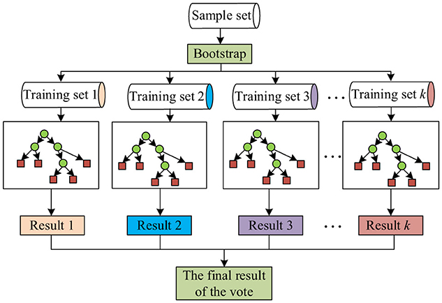
Figure 2. Random forest feature selection process diagram.

Considering that the transmission line loss rate is easily affected by environmental factors, social factors, load rate level, and other factors, referring to these characteristic variables' influence is necessary when predicting the short-term line loss rate. However, the category and data dimension of the characteristic variables cannot be directly estimated, which also has a great impact on the complexity of calculating the line loss rate prediction model. Therefore, analyzing the degree of influence on the line loss rate is necessary, as is appropriately eliminating the characteristic variables with less influence, which is conducive to improving the calculation efficiency and prediction accuracy of the prediction model. In this article, the influencing factors' characteristics are sorted and screened before predicting the online loss rate. First, the influencing factors are shown in Table 1.

Table 1

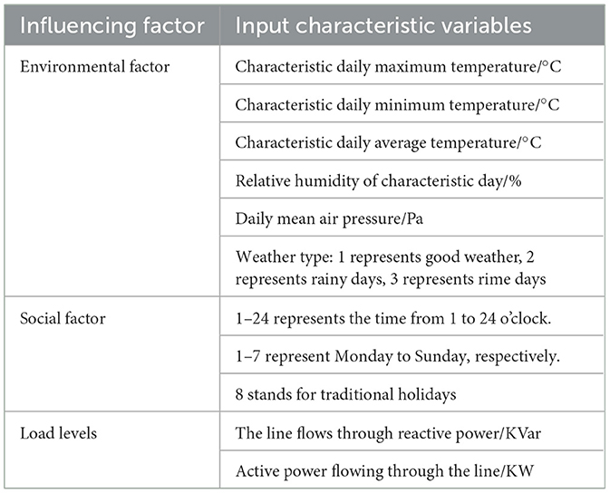
Table 1. Selection table of influencing factors.

Next, the importance of each factor affecting the line loss rate is analyzed, and the influencing factors are preprocessed. The 11 characteristic variables in Table 1 are selected as data input, and the importance of each characteristic quantity is analyzed, as shown in Figure 3.

Figure 3

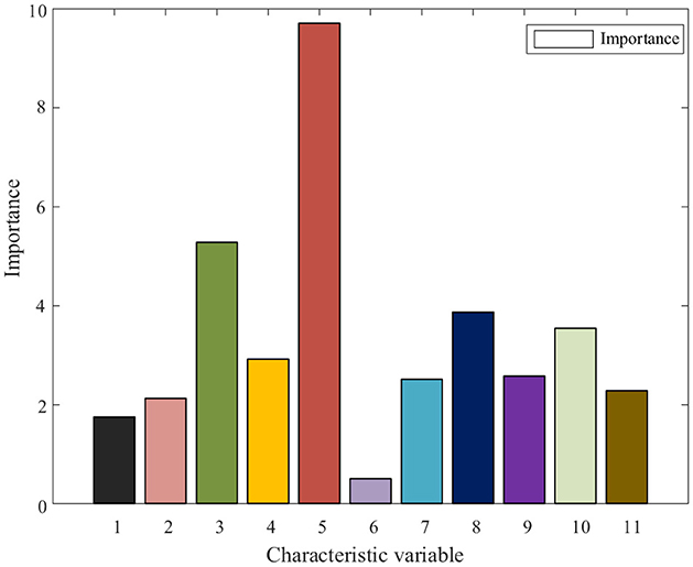
Figure 3. Comparison chart of the importance of characteristic variables.

In Figure 3, the characteristic variables are labeled as follows: 1 corresponds to the highest daily temperature; 2, to the lowest daily temperature; 3, to the daily average temperature; 4, to the weather type; 5, to the working day; 6, to the daily average air pressure; 7, to relative humidity; 8, to the active power of the line; 9, to the line reactive power; 10, to the rest day; and 11, to the holiday. It can be seen that the importance of each characteristic variable affecting the line loss rate is different. Considering that the importance of the characteristic daily average air pressure with the least influence is < 0.1, to reduce the dimension of the input characteristic variable matrix and simplify the calculation, the daily average air pressure with the importance of the influencing factors < 0.1 is eliminated, and the remaining 10 characteristic variables are used together as the input of the line loss rate prediction model.

4 Short-term line loss rate prediction model based on RF-CNN-LSTM

4.1 CNN

A CNN model (Jianji et al., 2022) is a neural network model proposed by LeCun in 1989. The model's performance is better in feature extraction and can supplement the shortcomings of other network models. The composition of the CNN model is as follows:

1. Input layer: Its function is to input the original data set.

2. Convolution layer: The convolution operation is used to extract the features that affect the line loss rate into features more in line with the prediction model. The convolution kernel is equivalent to an input matrix, which can perform convolution operations on data in different input regions. Finally, it is multiplied by the coefficient matrix of the convolution kernel to obtain a convolution matrix, which is the feature variable matrix. Therefore, different convolution kernels can obtain different convolution feature matrices. Therefore, compared with the original features, the previously mentioned convolution features obtained are more effective and can help the model have higher performance. The basic equation of the convolution layer operation is shown in Equation 14:

$\begin{array}{ll}{C}^l=ReLU(Wx+b),& (14)\end{array}$

where C^l is the output feature of the convolutional layer l, ReLU( ) is the activation function, x is the input of the convolution layer, W is the weight of the convolutional layer, and b is bias.

3. Pooling layer: Its role is to reduce the data dimension. This is a sub-sampling technique, which is similar to the convolution operation, and extracts the features of each convolution feature block through a small sliding window to output new features. Therefore, the role of pooling is not only to summarize the previous convolution features but also to filter out the bad features, thus improving the stability of the model. Therefore, to reduce the parameter types of the convolutional layer and the dimension of the data set, we calculate the average and maximum values of the feature variable data, referred to as average pooling and maximum pooling. The calculation formula of the maximum pooling layer is shown in Equation 15:

$\begin{array}{ll}{x}_j^l=f\left({\beta }_j^{l}down\left(x_j^{l-1}\right)+b_j^l\right),& (15)\end{array}$

where down()denotes the maximum pooling sampling function, $x_j^l$ represents the input feature map of the data j of the convolutional layer l, and ${\beta }_j^l$ is deviation.

4. Full connection layer: After classifying the processed data, the output results are sent to the next network model.

5. Output layer: This represents the output line loss rate value.

The structure of the CNN is shown in Figure 4.

Figure 4

Figure 4. Convolutional neural network (CNN) structure diagram.

4.2 LSTM

LSTM has a good performance in processing time-series data. The data involved in the line loss rate are time-series data, such as temperature, weather forecast data, daily load rate, and so on, so the prediction of the line loss rate is widely used.

LSTM is a chain-structured neural network, which is unique in that it adds a gate structure for the data-storing state. Due to the structural characteristics of the input gate, forgetting gate, and output gate, when there is an error in the activation function, the important information will still be iterated together and continue to be transmitted backwards, so there is no long-term dependence between the chain structures. The hidden layer chain structure of the LSTM neural network is shown in Figure 5.

Figure 5

Figure 5. Long short-term memory neural network hidden layer chain structure diagram.

In the chain's hidden layer are three gate structures: the input gate, the forgetting gate, and the output gate, as shown in Figure 6. Therefore, this layer can selectively retain a certain part of all data, rather than a single datum. The three gate structures also determine that it can accept the output of multilayer neurons.

Figure 6

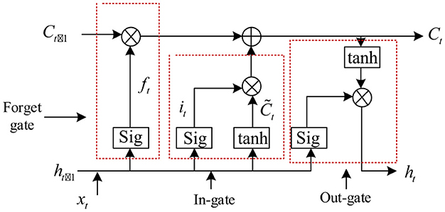
Figure 6. Long short-term memory neural network model structure diagram.

The role of the forgetting gate is to determine which useless information is received in the forgetting model. The forgetting gate combines the output h_t−1 of the hidden layer at time t−1 and the input x_t at time t. The three can be processed together by the activation function to obtain an arbitrary value of [0, 1]. When the number obtained is between 0 and 1, the data can be selectively retained. When the value is 1, the data are considered useful information, and all the information is retained. When the value is 0, all the data are considered useless information, and the information is forgotten. The calculation method of forgetting gate is as follows:

1. The forgetting gate takes the input x_t of time t and h_t−1 the output of time t−1 as the reference, and deletes the information from the storage unit. Its expression is shown in Equation 16:

$\begin{array}{ll}{f}_t=\sigma (w_{fh}\times h_{t-1}+w_{fx}\times x_t+b_f),& (16)\end{array}$

where h_t−1 is the offset of the forgetting gate, f_t is the state of the forgetting gate, σ() is the activation function, and w_fh and w_fx are the weight matrices of the forgetting gate.

2. The information stored in the storage unit is determined. Its expression is shown in Equation 17:

$\begin{array}{l}{i}_t=\sigma (w_{ih}\times h_{t-1}{+w}_{ix}\times x_t{+b}_i)\\ {\tilde{c}}_t=tanh(w_{\tilde{c}h}\times h_{t-1}{+w}_{\tilde{c}h}\times x_t{+b}_{\tilde{c}}),& (17)\end{array}$

where w_ih, w_ix, and $w_{\tilde{c}h}$ are the weight matrices of the input gate; i_t is the state of the input gate; tanh() and σ() are activation functions; ${\tilde{c}}_t$ is the state of the candidate element; and b_i and $b_{\tilde{c}}$ are the offsets of the input gate.

3. Combined with the state of the forgetting gate and the input gate, the unit state C_t is updated. Its expression is shown in Equation 18:

$\begin{array}{ll}{C}_t=f_t·C_{t-1}+i_t·{\tilde{c}}_t,& (18)\end{array}$

where C_t−1 is the element state of time t−1.

4. In the unit state at time t, the state O_t of the output gate is updated. Its expression is shown in Equation 19:

$\begin{array}{ll}{O}_t=\sigma (w_{oh}·h_{t-1}+w_{ox}·x_t+b_o),& (19)\end{array}$

where w_oh and w_ox are the weight matrices of the output gate and b_o is the offset of the output gate.

5. The final output of the output gate is determined. Its expression is shown in Equation 20:

$\begin{array}{ll}{h}_t=O_t·tanh(C_t),& (20)\end{array}$

where h_t is the output at time t, that is, the line loss rate value.

4.3 Construction of short-term line loss rate prediction model based on the RF-CNN-LSTM

4.3.1 RF-CNN-LSTM prediction model construction

To predict the change of transmission line loss rate more accurately, a CNN-LSTM combined model is constructed as shown in Figure 7. Its steps are as follows: The first step is to input the processed data to the model through the input layer. The second step is to extract the important information in the data through the convolution layer and reduce the dimension of the pooling layer to obtain the output data. The third step is to train the output data by the LSTM layer. The fourth step is to enter the output layer to obtain the output value.

Figure 7

Figure 7. Convolutional neural network (CNN)–long short-term memory (LSTM) model structure diagram.

When using the CNN-LSTM model to predict the short-term line loss rate value, the CNN neural network is first used to extract the feature quantity of the line loss rate influencing factors, and the original data set is divided into a training set (80%) for training the model. This process allows the model to find the correlation between the line loss rate and the influencing factors so that the model becomes more suitable for line loss rate prediction, and the test set (20%) is used to test the model's accuracy. LSTM can not only fully obtain the time-series characteristics of line loss rate data through memory function but also accurately grasp the non-linear relationship between input data and line loss rate and has higher accuracy when predicting transmission line loss rates.

The prediction model based on the RF-CNN-LSTM is constructed in the following discussion, and the prediction process is shown in Figure 8.

Figure 8

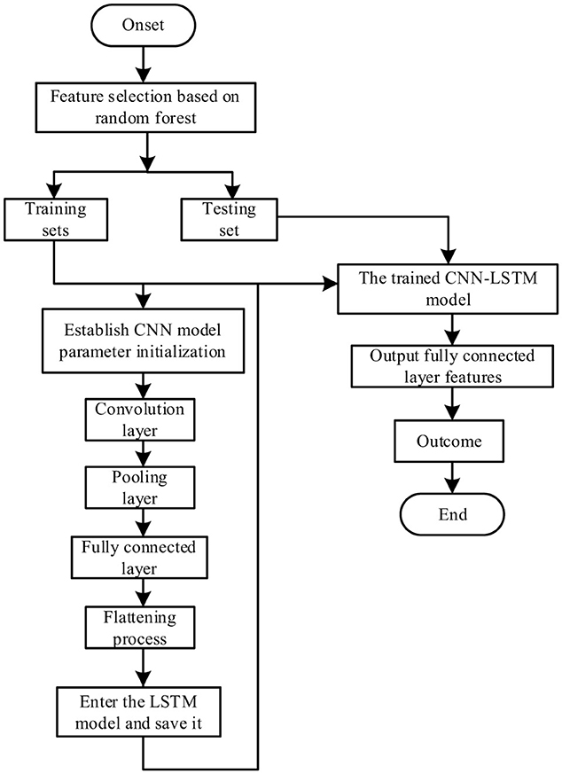
Figure 8. Random forest convolutional neural network (CNN)–long short-term memory (LSTM) model prediction flowchart.

In summary, the steps to establish the RF-CNN-LSTM short-term line loss rate prediction model are as follows:

1. Data acquisition and pre-processing: The data for transmission line loss rate, environmental factors, and time on the characteristic day are collected, and the missing data completion and distortion data processing are carried out. Finally, the data are normalized to the same order of magnitude.

2. Data partitioning: To make the model fully trained, the original data set is usually divided into a training set (80%) and a test set (20%). The former is used to train the prediction model, and the latter is used to test the model training results and prediction accuracy.

3. Feature extraction: The training set is used to train the CNN model for data feature extraction and finally input into the LSTM model through the convolutional layer, the pooling layer, and the fully connected layer for line loss rate prediction.

4. Model evaluation: The training fitting effect of the training set was observed, and the prediction performance of the model was evaluated using the test set.

5. Analysis of prediction results: The measured parameters are input into the model, and the error evaluation index is used to compare the predicted line loss rate with the real value to judge the model's prediction accuracy and evaluate the prediction model's advantages and disadvantages.

4.3.2 RF-CNN-LSTM hybrid architecture design

This article proposes a hybrid architecture of the RF-CNN-LSTM. The system adopts the RF-CNN-LSTM three-stage processing flow, as follows:

1. RF feature selection layer: The key influencing factors are screened, and the optimized feature subset is constructed. According to Section 3, before the data are input into CNN-LSTM, an RF is used to evaluate and select the importance of features, and the features after RF screening are reconstructed into three-dimensional tensors as CNN input.

2. CNN spatial feature extraction module: According to Section 4.1, the convolution layer and pooling layer are determined, and the data after convolution and pooling are used as the input of the LSTM. In this article, the line loss rate data of the previous period is used to predict the line loss rate of the next time point. Therefore, the line loss rate data need to be processed by a sliding window. The step size of the sliding window is 1, and the length is artificially set to obtain the trajectory matrix as input. To preserve the time information as much as possible, the convolution kernel should be as small as possible. Moreover, the short-term fluctuations of line loss rate are more critical and should focus on local segments. Therefore, the convolution kernel size is unified to 3 × 3.

3. LSTM timing modeling module: Capture the dynamic evolution law of the line loss rate. The fully connected layer converts the spatial features output into time-series vectors using a CNN. According to Section 4.2, the LSTM layer outputs data through the forgetting gate to complete the prediction.

The specific number of convolution kernels, convolution kernel size, step size, and other information are shown in Table 2.

Table 2

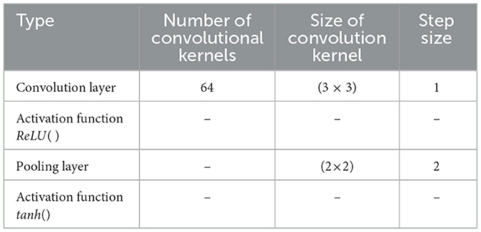
Table 2. Internal parameters of convolutional neural network–long short-term memory model.

5 Experimental prediction analysis

5.1 Short-term line loss rate prediction error evaluation index

The indicators of conventional error analysis are root mean square error (RMSE), mean absolute error (MAE), and mean square error (MSE). Its calculation expression is shown in Equations 21–23:

$\begin{array}{ll}RMSE=\sqrt{\frac{1}{n}{\displaystyle \sum _{i=1}^n}{(x_i-\overline{x_i})}^2}& (21)\end{array}$

$\begin{array}{ll}MAE=\frac{1}{n}{\displaystyle \sum _{i=1}^n}|x_i-\overline{x_i}|& (22)\end{array}$

$\begin{array}{ll}MSE=\frac{1}{n}{\displaystyle \sum _{i=1}^n}{(x_i-\overline{x_i})}^2.& (23)\end{array}$

The error curve is drawn by using the predicted relative error. The formula is as follows:

$\begin{array}{ll}RE=\left|\frac{x_i-\overline{x_i}}{x_i}\right|& (24)\end{array}$

where n is the number of samples in the test set, x_i is the actual value of the line loss rate at the time of the sampling i, and $\overline{x_i}$ is the predicted value of the line loss rate at sampling i. The smaller the value of the error evaluation index is, the more the predicted value fits the real value, and the higher the accuracy of the model prediction is.

5.2 Experimental condition

The short-term line loss rate prediction is mainly to predict the line loss rate within the next 2 h to 2 weeks. Considering the maximum margin, this experiment will predict the line loss rate within 2 weeks. The data set of transmission line loss rate for 15 days from May 1 to May 15, 2024, is selected, and the line loss rate and characteristic variables are collected every 60 min. The first 12 days were the training set, and the next 3 days were the test set. After training the RF-CNN-LSTM model, the line loss rate data for the next 3 days are predicted and analyzed.

Based on Section 4.3, the parameter settings of the RF-CNN-LSTM model are shown in Table 3. The initial learning rate is set to 0.001, and the dropout rate is set to 0.2 in the LSTM layer to prevent overfitting.

Table 3

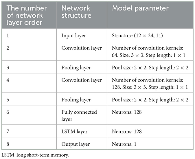
Table 3. Model parameter settings.

After many experiments, two convolutional layers and two maximum pooling layers are selected. This setting can help CNN better extract the feature relationship between the line loss rate and the influencing factors. The advantages are as follows:

1. Setting two convolutional layers and the maximum pooling layer can extract the higher-dimensional relationship between the line loss rate and the characteristic variables of the influencing factors and enhance the expression ability of the model after learning.

2. The small convolution kernels of 64 and 128 are used to extract the main features as much as possible, and there is no overfitting. It will reduce the computational burden of the model, ensure accuracy, and improve the prediction efficiency.

3. The maximum pooling layer can help reduce the dimension of feature quantities, abandon redundant data, and only extract important features, thereby reducing the amount of calculation and making the model more robust.

4. Using ReLU( ) as the activation function can enhance the learning ability of the CNN, which is helpful to activate larger positive neurons and inhibit negative neurons. At the same time, the activation function also has a good performance in fitting complex non-linear problems.

5.3 Experimental result analysis

5.3.1 Ablation experiment

An RF is introduced based on the CNN-LSTM to obtain the RF-CNN-LSTM model. An ablation experiment is carried out using the preceding model, and the results are shown in Table 4.

Table 4

Table 4. Ablation experimental results.

According to Table 4, compared with the CNN-LSTM model, the RF-CNN-LSTM model's RMSE increases by 13.6%, its MSE by 9.6%, its MAE by 14.65%, and its MSE by 25.4%. When MAE is used as the evaluation standard of neural networks, the RF-CNN-LSTM has a better overall prediction effect on the short-term line loss rate. The RF algorithm can eliminate redundant features, and the overall accuracy of the RF-CNN-LSTM model is significantly improved after focusing on the key influencing factors and selecting the feature quantity of RF. In addition, the RF-CNN-LSTM performs well on the MSE and RMSE indicators, and the prediction results are more stable.

5.3.2 RF-CNN-LSTM model experiment and analysis

The test results are shown in Figures 9, 10.

Figure 9

Figure 9. The fitting effect of random forest–convolutional neural network–long short-term memory model training set samples.

Figure 10

Figure 10. Random forest–convolutional neural network–long short-term memory line loss rate prediction results.

The error evaluation indexes, RMSE, MAE, and MSE, proposed in Section 5.1 are used to analyze the error of the prediction results of the RF-CNN-LSTM model. According to the calculation, the error evaluation indexes of the RF-CNN-LSTM model can be obtained, specifically RMSE = 0.09753, MAE = 0.13807, and MSE = 0.00951.

It can be seen from Figure 9 that for the RF-CNN-LSTM model training set samples, the overall fitting effect is good. However, when the number of training set samples is in the 20–50 range, the peak fitting effect of the RF-CNN-LSTM model is not good, and the error is ~15%. As the number of training set samples increases, the error gradually decreases. This shows that when the sample size is insufficient, the model has difficulty fully learning the spatial and temporal characteristics and noise patterns contained in the peaks, resulting in limited generalization ability and error. When the training data are sufficient, the RF-CNN-LSTM components can be collaboratively optimized, which effectively alleviates the risk of overfitting and improves the accuracy of peak fitting.

From Figure 10, it can be seen that when the RF-CNN-LSTM model is used for actual testing, the measured value is also close to the true value. However, the prediction error at the peak of the actual prediction is ~7%, and the error is relatively large. This may be related to the strong volatility of line loss rate data, the granularity of line loss rate data, and the initial parameter setting during this period.

5.3.3 Contrast experiment

To further prove the superiority of the prediction method proposed in this paper, the same data sets are input into the RF-CNN-LSTM model and the RF-CNN-SVM model, respectively. The test results are shown in Table 5 and Figures 11, 12.

Table 5

Table 5. Ablation experimental results.

Figure 11

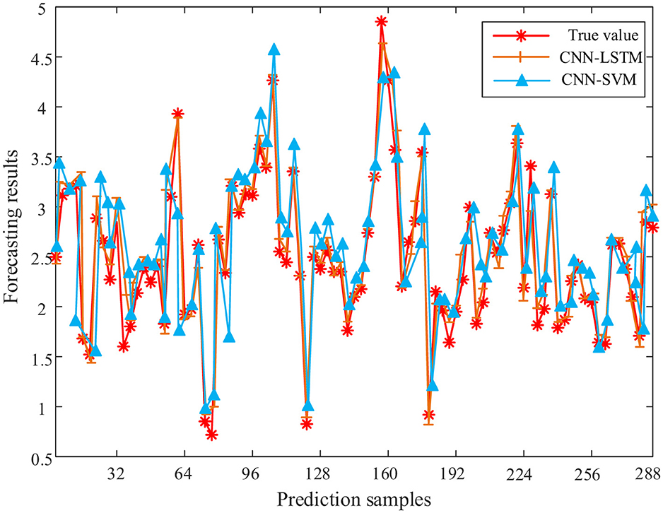
Figure 11. Random forest–convolutional neural network–long short-term memory model and random forest–convolutional neural network–support vector machine model training set fitting effect comparison chart.

Figure 12

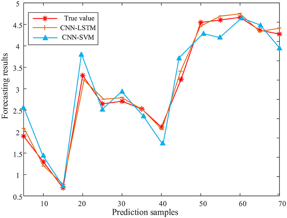
Figure 12. Comparison of random forest–convolutional neural network–long short-term memory and random forest–convolutional neural network–support vector machine models in predicting line loss rate. CNN, convolutional neural network; LSTM, long short-term memory; SVM, support vector machine.

It can be seen from Table 5 that the error evaluation indexes of the RF-CNN-SVM model are as follows: RMSE = 0.10242, MAE = 0.15129, and MSE = 0.01049. Compared with the RF-CNN-LSTM model, all error evaluation indices are significantly increased. Compared with the RF-CNN-SVM model, the RMSE of the RF-CNN-LSTM model proposed in this article is reduced by 4.78%, the average absolute error is reduced by 8.7%, and the mean square error is reduced by 9.34%.

It can be seen from Figure 11 that the RF-CNN-SVM model training set has a poor fitting effect, and the fitting effect at the peak and trough is worse than that of the RF-CNN-LSTM model. It can be seen from Figure 12 that the CNN-SVM model has a poor fitting effect on the short-term line loss rate, and the prediction results at the peaks and troughs are quite different from the real values. The RF-CNN-LSTM model is closer to the real value than the RF-CNN-SVM model. The comparison of the two prediction results can highlight the advantages of RF-CNN-LSTM in predicting short-term line loss rate. In summary, the RF-CNN-LSTM model proposed in this paper has more advantages in predicting short-term line loss rate.

6 Conclusion

In this article, an RF algorithm is used to sort the influencing factors of line loss rate according to their importance, and the daily average air pressure with the proportion of influencing factors < 0.1 is removed, which can reduce the data dimension and improve the reliability and speed of model training. Considering that the feature variables extracted by the input layer of the traditional method are not complete, a CNN was used to extract the feature variables. Then the LSTM neural network was selected for prediction. To verify the accuracy of the prediction results, the SVM algorithm is set up for synchronous prediction as a comparative experiment. The results show that the CNN-LSTM neural network prediction results are more accurate.

Data availability statement

The original contributions presented in the study are included in the article/supplementary material, further inquiries can be directed to the corresponding author.

Author contributions

LJ: Conceptualization, Writing – original draft, Writing – review & editing. CL: Writing – original draft, Conceptualization, Writing – review & editing. WQ: Writing – review & editing, Data curation, Writing – original draft. CX: Writing – review & editing, Writing – original draft, Data curation. JY: Writing – review & editing, Formal analysis. JS: Formal analysis, Writing – review & editing.

Funding

The author(s) declare that financial support was received for the research and/or publication of this article. The work of this article was funded by the science and technology project of China Southern Power Grid. The project number is 030400KC23120031 (GDKJXM20231501). The funder was not involved in the study design, collection, analysis, or interpretation of data, the writing of this article, or the decision to submit it for publication.

Acknowledgments

This article is grateful to China Southern Power Grid Power Grid Project for funding.

Conflict of interest

LJ, CL, and WQ were employed by Zhuhai Power Supply Bureau of Guangdong Power Grid Co., Ltd. JY and JS were employed by Dongfang Electric Academy of Science and Technology Co., Ltd.

The remaining author declares that the research was conducted in the absence of any commercial or financial relationships that could be construed as a potential conflict of interest

Generative AI statement

The author(s) declare that no Gen AI was used in the creation of this manuscript.

Publisher's note

All claims expressed in this article are solely those of the authors and do not necessarily represent those of their affiliated organizations, or those of the publisher, the editors and the reviewers. Any product that may be evaluated in this article, or claim that may be made by its manufacturer, is not guaranteed or endorsed by the publisher.

References

Guo, Q., Guo, Q., Guo, Q., He, Z., He, Z., and Wang, Z. (2023). Prediction of monthly average and extreme atmospheric temperatures in Zhengzhou based on artificial neural network and deep learning models. Front. For. Glob. Change 6:1249300. doi: 10.3389/ffgc.2023.1249300

Crossref Full Text | Google Scholar

Guo, Q., He, Z., and Wang, Z. (2024a). Monthly climate prediction using deep convolutional neural network and long short-term memory. Sci. Rep. 14:17748. doi: 10.1038/s41598-024-68906-6

PubMed Abstract | Crossref Full Text | Google Scholar

Han, H., Kun, S., and Da, L. (2018). Research on hourly load forecasting of power system based on random forest. Smart Power 46, 8–14.

Google Scholar

Jianhua, Y., Daqiang, X., Huixin, L., Mingqiong, Y., and Benshun, Y. (2020). Prediction of 1000kV extra high voltage line loss based on improved grey correlation analysis and LSTM. Electr. Technol. 19, 131–136.

Google Scholar

Jianji, R., Huihui, W., Zhuolin, Z., Tingting, H., Yongliang, Y., Jiquan, S., et al. (2022). Ultra-short-term power load forecasting based on CNN-BiLSTM-attention. Power Syst. Protect. Control 50, 108–116.

PubMed Abstract | Google Scholar

Kim, T., and Cho, S. (2019). Predicting residential energy consumption using CNN-LSTM neural networks. Energy 18, 72–81. doi: 10.1016/j.energy.2019.05.230

Crossref Full Text | Google Scholar

Liao, Y., En, W., Li, B., Zhu, M., Li, B., Li, Z., et al. (2023). Research on line loss analysis and intelligent diagnosis of abnormal causes in distribution networks: artificial intelligence based method. Comput. Sci. 9, 53–59. doi: 10.7717/peerj-cs.1753

PubMed Abstract | Crossref Full Text | Google Scholar

Lin, X., Hongwei, L., Yue, Y., and Hailin, Z. (2021). Line loss calculation method based on K-Means clustering and improved multi-classification relevance vector machine. J. Electr. Eng. 16, 62–69.

Google Scholar

Qi, A., Zhanbin, W., Guoqing, A., Zheng, L., He, C., Zheng, L., et al. (2022). Non-invasive load identification method based on random forest-genetic algorithm-extreme learning machine. Sci. Technol. Eng. 22, 1929–1935.

Google Scholar

Ruiming, N., and Jiayu, R. (2021). Method for judging abnormal line loss rate in station area based on data analysis. Electr. Technol. 8, 136–139.

Google Scholar

Xiaoke, Y., Tianren, Z., Yuping, H., Xianfu, G., and Bo, P. (2023). Analysis of the impact of low-carbon and high-quality development of Guangdong Electric Power on coal demand. Guangdong Electric Power 36, 1–10.

Google Scholar

Yinbiao, S., Guoping, C., Jingbo, H., and Fang, Z. (2021b). Research on constructing a new power system framework with new energy as the main body. China Eng. Sci. 23, 61–69.

Google Scholar

Yinbiao, S., Liying, Z., Yunzhou, Z., Yaohua, W., Gang, L., Bo, Y., et al. (2021a). Research on the carbon peak and carbon neutralization path of China 's electric power. China Eng. Sci. 23, 1–14. doi: 10.15302/J-SSCAE-2021.06.001

Crossref Full Text | Google Scholar

Yingchun, W., Yuxuan, Z., Zan, W., Jianhua, Y., Hongbin, L., and Dongyue, M. (2020). Multi-parameter correction algorithm for transmission line loss. J. Electric Power Sci. Technol. 35, 126–131.

Google Scholar

Yiwen, W. (2022). Research on Pipe Burst Detection of Water Supply Network Based on RF-LSSVM Interactive Prediction. Kunming: Kunming University of Science and Technology.

Google Scholar