

- The Smith-Kettlewell Eye Research Institute, San Francisco, CA, USA
Although brain imaging methods are highly effective for localizing the effects of neural activation throughout the human brain in terms of the blood oxygenation level dependent (BOLD) response, there is currently no way to estimate the underlying neural signal dynamics in generating the BOLD response in each local activation region (except for processes slower than the BOLD time course). Knowledge of the neural signal is critical if spatial mapping is to progress to the analysis of dynamic information flow through the cortical networks as the brain performs its tasks. We introduce an analytic approach that provides a new level of conceptualization and specificity in the study of brain processing by non-invasive methods. This technique allows us to use brain imaging methods to determine the dynamics of local neural population responses to their native temporal resolution throughout the human brain, with relatively narrow confidence intervals on many response properties. The ability to characterize local neural dynamics in the human brain represents a significant enhancement of brain imaging capabilities, with potential applications ranging from general cognitive studies to assessment of neuropathologies.
Introduction
The basic capability of functional magnetic resonance imaging (fMRI) is mapping the spatial organization of the cortical and subcortical responses throughout the brain to a variety of stimulus and behavioral paradigms. The blood oxygen level dependent (BOLD) signal measured by fMRI is often considered to have high spatial resolution (up to a quarter of a million voxels), but low temporal resolution (0.5–5 s) relative to other methods for mapping human brain function (such as high-density EEG analysis). Of course, even the BOLD spatial resolution is low relative to single-unit neurophysiological recoding, but this is largely attributable to the signal/noise ratio. In-plane spatial resolution for functional imaging as high as 150 μm has been reported at 9.4 T in cat cortex (Harel et al., 2006) and less than 1 mm × 1 mm × 1 mm voxels have been achieved in human (Barth and Norris, 2007). As improved technologies come on line, such high spatial resolution is expected to be continually increased, as exemplified by the “inverse imaging” approach of Lin et al. (2008).
The temporal limit is not so tractable. The inherent time constants of the BOLD signal are about 5 s, several orders of magnitude slower than the neural signal that is driving it, even for the most recent fast acquisition protocols (Lin et al., 2008; Grotz et al., 2009). For a reasonable recording time and voxel size (e.g., 3 mm × 3 mm × 3 mm) the signal/noise ratio even for the most effective stimuli rarely exceeds 20:1. At such signal/noise ratios, deconvolution of the BOLD response can improve its temporal resolution by about a factor of 5 (Glover, 1999; Logothetis, 2003). However, that leaves the temporal resolution for the underlying neural signal at about 1 s, which is far short of what is required to measure typical neural delays. Estimation of single-parameters of the waveform, such as response delay alone, can improve the temporal resolution for the neural signal delays to 100 ms or better for narrowly targeted brain regions (Menon et al., 1998; Henson et al., 2002) but this requires the assumption that the BOLD signal has a unitary waveform, which is often not the case (Aguirre et al., 1998; d’Avossa et al., 2003; Handwerker et al., 2004; Likova and Tyler, 2007). Even minor deviations from a stable waveform violate the assumptions of such single-parameter analysis and invalidate the delay measure.
Indeed, most commonly used fMRI analysis techniques, such as the SPM analysis package, employ the convolution approach. Convolution is based on the assumption of a unitary BOLD waveform kernel that generates the straightforward prediction of the BOLD response waveform for any stimulus type or duration in any brain area. In fact, however, major deviations from a standard BOLD waveform may be found, even in the same cortical regions, for variations in stimulus conditions. d’Avossa et al. (2003), for example, reported strong differences in waveform when the response to the motion or color of a cue/stimulus pairing was modulated by attention. Such local waveform differences must derive from differences in the neural signals driving the BOLD activation, since the metabolic and hemodynamic processes that mediate the paramagnetic signals should be invariant within a given cortical region.
To study the neural involvement in generating differential BOLD response waveforms within the same cortical regions, Likova and Tyler (2007) developed an “instantaneous stimulus paradigm” to evoke BOLD responses to instantaneous stimulus transitions. It is typically assumed that, despite their perceptual differences, such “instantaneous” stimuli would all generate the same BOLD waveform (effectively equivalent to the hemodynamic response function, HRF) for all different stimulus types. Thus, revealing any significant deviation from that prediction in the BOLD waveform elicited in one and the same cortical area can contribute to revealing the specifics of the underlying neural processing and enhance the understanding of the recurrent network of extended perceptual responses to complex stimulus configurations. Indeed, the instantaneous stimulus paradigm generated a wide variety of BOLD waveforms. Moreover, the data show dramatic differences in the BOLD waveforms properties (e.g., latency, sign, amplitude, and width) even within the same brain areas as a function of the stimulus type. As there can be no vascular heterogeneity within the same area, these dramatic waveform variations must be attributed to differences in the underlying neural dynamics, not to spatial variations in the HRF. These results further imply that fMRI signals contain much more information about the neural processing than is commonly appreciated, and thus have the potential to capture them through an appropriate approach.
However, there is at present no method of transcending the BOLD temporal limitations in order to estimate the dynamics of the neural signals underlying the measured fMRI waveforms. The goal of the temporal analysis we propose is therefore to provide a method for the time-resolved estimation of the neural signals underlying the particular characteristics of the temporal BOLD waveforms for a particular stimulus processed by a particular cortical region. The philosophy of this approach is to utilize the information available from neurophysiological studies of the neural population dynamics and biochemical studies of the metabolic pathway coupling to the measurable blood response to provide Bayesian priors as to the likely temporal structure of the component neural signals. We propose a non-linear dynamic forward optimization (NDFO) approach to provide a compact account of the measured waveform with the minimal number of neural predictors, based on prior knowledge of the expected temporal properties of neural signals and of their consequent metabolic demand. This approach is reminiscent of the spectral analysis of the composition of stars, in which each chemical element has a characteristic pattern of emission lines (the Bayesian priors) and the net spectrum is the sum of an unknown mixture of these predetermined patterns. The result is the ability to specify the prevalence of each element in the otherwise inaccessible star. In the case of the neural signals, the goal is to estimate the amplitude and time course of each of the neural components whose metabolic effects, when summed, account for the measured BOLD waveform for a particular stimulation condition and cortical region. Here the predictors are non-linear because there is a non-linear relationship between the neural responses and the metabolic demand that they generate, but the summative property of the paramagnetic signals throughout a voxel implies that we can assume that the component metabolic demands sum linearly together.
Theoretical Overview
To start the analysis, we may develop a specific model structure of the processes leading to the BOLD paramagnetic signal of fMRI recordings. We note that this model is focused on the non-linearities that are likely to affect the process of estimating neural responses from BOLD waveform properties, but simplifies aspects of the biophysical processes that will not be resolvable by the NDFO technique. As such, it is substantially elaborated relative to the linear convolution analyses of Friston (1997) and Friston et al. (1998, 2000), but somewhat condensed in comparison with the recent biophysical/metabolic derivations of Mechelli et al. (2001), Buxton et al. (2004), or Sotero and Trujillo-Barreto(2007, 2008).
We will treat the neural responses within each voxel as generated by sets of homogeneous populations with similar signal waveforms Ni(t) within each population (Figure 1). Each neural response then generates a local metabolic demand Mi(t) that may have a non-linear relationship to the neural signal waveform (Chatton et al., 2003).
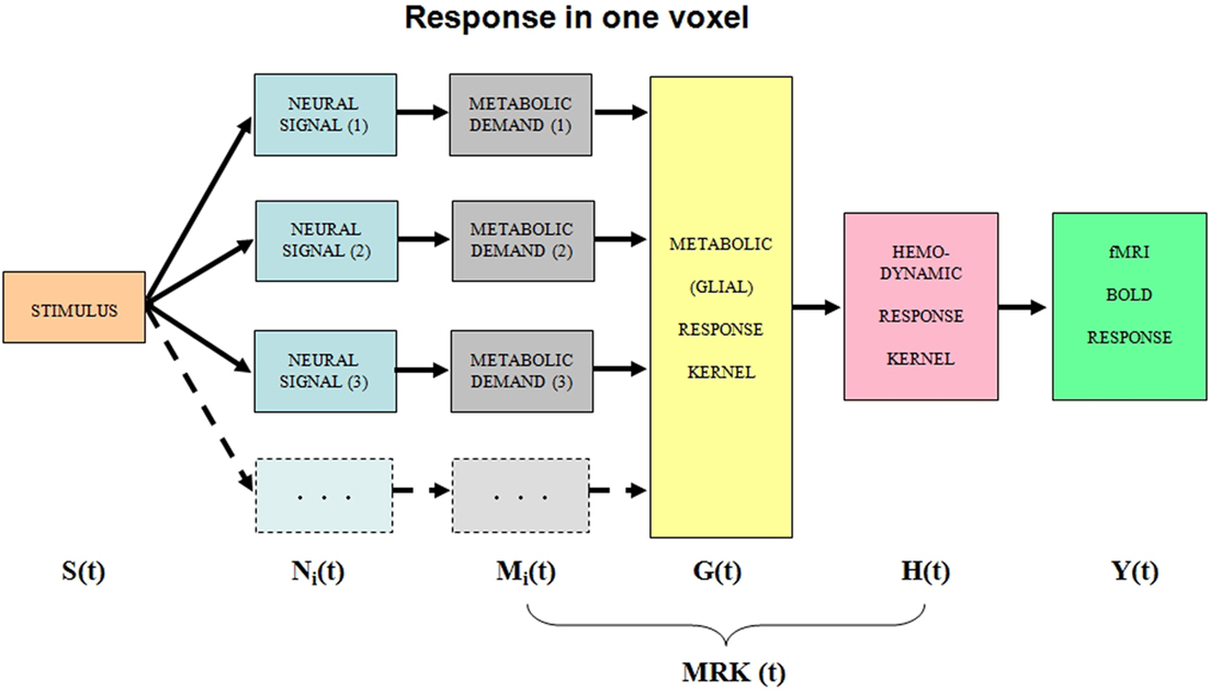
Figure 1. Block diagram of the main processing stages that lead up to the BOLD signal. The i subscript indicates that the stage incorporates multiple components within the voxel. See text for details.
The metabolic demand has been shown to have a short time course, on the order of the membrane response to a single pre-synaptic spike (Magistretti and Pellerin, 1999; Magistretti, 2009). The integrated metabolic demands are met primarily by the astrocytes, which integrate the required energy consumption over time and space and make a complementary oxygen demand G(t) on the adjacent vasculature. The hemodynamic processes H(t) provide the requisite oxygen exchange to replenish the energy depletion in the astrocytes and other intermediary processes. The fMRI BOLD analysis provides an estimate Y(t) of the ratio of oxygenated to deoxygenated hemoglobin in the blood complement of a given voxel. The post-neural processing stages are often modeled as a linear hemodynamic response kernel convolved with the presumed neural signal. However, this approach overlooks the key role of the pre-hemodynamic processes of the glial and other intermediaries. To incorporate the contributions of these intermediary processes, we will term it a “metabolic response kernel” (MRK1) incorporating both the glial and hemodynamic components of the metabolic recovery processes. The MRK will be convolved with a non-linear transform of the presumed neural signal to provide an estimate of the neural metabolic demand that is being met by the combined glial and hemodynamic metabolic response. The fMRI analysis also has a finite dynamic response time, but it will be treated as incorporated in the MRK of the glial/hemodynamic response. The formal equations linking the processing stages in Figure 1 are provided in Table 1.
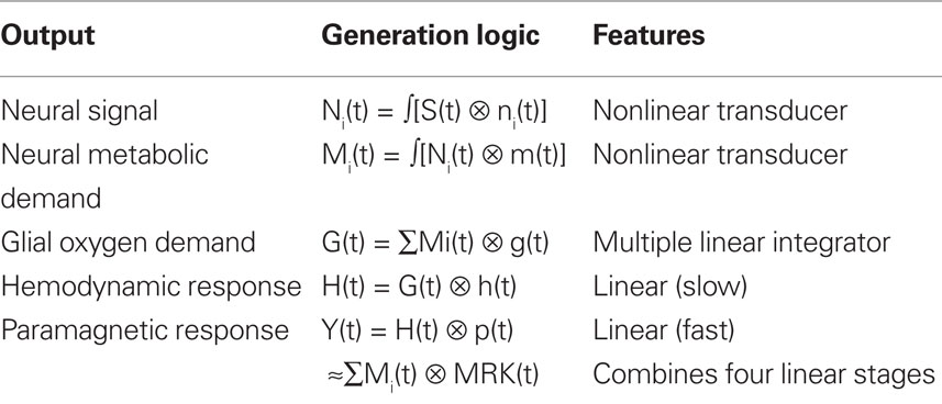
Table 1. Mathematical model of the linear and nonlinear operations involved in the generation of the BOLD signal from the input stimulus, S(t).
Direct Forward Modeling Approaches
A few previous studies have made estimates of the effects of different neural models on the form of the BOLD response dynamics. For example, Mechelli et al. (2001) report a simulation study of the estimated regional cerebral blood flow (rCBF) and BOLD signals as a function of the duration, onset asynchrony, and relative amplitudes of two brief stimuli. They included a basic model of neuronal dynamics and varied one parameter of this model – the amplitude of a slow late transient – to show its effect on the simulated BOLD responses. This exercise constitutes an unvalidated forward model of the effect of only one parameter of a simulated neural response. However, what they offer as the analysis of the effects on the BOLD waveform is described (incomprehensibly) as “the BOLD parameter estimates,” which is actually a single-valued function with no specification of which parameter(s) is/are being estimated. Since no comparison is made with empirical data or their noise limitations, the fact that this study includes a proposed model for the neural dynamics does not qualify it as a validated procedure for estimating the neural population dynamics underlying the local BOLD signals (which is the goal of our study).
Buxton et al. (2004) extend their balloon model of the hemodynamic response leading to the BOLD signal by proposing a model of the neural response to account for the temporal non-linearity in BOLD responses as a function of duration. This neural response incorporates a slow subtractive inhibitory component to the net neural signal, which has the effect of producing a neural response consisting of an initial transient followed by a sustained plateau. Model responses for three kinds of stimuli – a single short pulse, two short pulses, and one long pulse, are offered as a demonstration of the properties of this model. As with Mechelli et al. (2001), no attempt is made to compare the model outputs with actual BOLD recordings, so the Buxton et al. (2004) study again does not qualify as a validated procedure for estimating the neural population dynamics underlying the local BOLD signals.
Both Mechelli et al. (2001) and Buxton et al. (2004) include parameters intended to account for the temporal non-linearity of short-duration responses (which do not fall linearly as response duration is reduced; Boynton et al., 1996; Birn et al., 2001). Both studies demonstrate the required lack of reduction in a single example of a short-duration response, but neither study provides a validation of either the waveform or the amplitude response function relative to empirical BOLD data. In principle, either model could provide a platform for such validation or the further estimation of the dynamics of the underlying neural population response, but they neither do so nor suggest procedures by which such estimation could be achieved.
Stepwise Incremental Estimation of the Neural Dynamics
Quantitative estimation of the temporal transients underlying BOLD responses can be achieved by the use of an appropriate set of temporal duration stimuli, such as the temporal summation study reported in Birn et al. (2001). Their stimuli consisted of counterphasing checkerboard patches with durations increasing in factors of 2 from 0.5–2 s (together with a 20-s duration stimulus). The key result was that the BOLD response amplitudes did not increase proportionately with stimulus duration. (A proportionate increase would be expected under a general linear model (GLM) of linear summation with a neural response of constant amplitude.) Instead, the amplitude showed little increase from the short durations, implying either a non-linear summation process or a disproportionate strength of neural signals for short-duration stimuli (Figure 2).
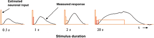
Figure 2. Neuronal input amplitude estimation by a box-car approximation to the presumed neuronal signal (red rectangles) that accounts for the BOLD responses (black line) as a function of the duration of a counterphase checkerboard stimulus. Reproduced from Bandettini and Ungerleider (2001).
Bandettini and Ungerleider (2001) proposed a discrete approximation analysis for the derivation of the implied neural signal in human cortex under the assumption that the integration process underlying the generation of the BOLD response was indeed equivalent to a linear convolution operation. To derive a crude estimate of the neural signal, they took the difference between integrated BOLD response areas for each successive pair of stimulus durations as an estimate of the amplitude of the neural signal for the time interval defined by the difference in stimulus durations (Figure 2), based on the (unstated) assumption that the neural response is fast enough to follow the stimulus exactly. This discrete approximation approach implied that the neural signal underlying these BOLD responses has a pronounced early transient followed by a sustained phase of stable amplitude out to 20 s (red box functions, Figure 2). The details of this transient, however, remained unresolved.
Non-Linear Dynamic Forward Optimization
In this section, we propose a more biophysically based development of the forward modeling approach that we term NDFO. Rather than simply characterizing the behavior of the BOLD waveform (Birn et al., 2001; Bandettini et al., 2002; d’Avossa et al., 2003; Fox et al., 2005; Grotz et al., 2009) or attempting to infer the potentially complex properties of the underlying neural mechanisms from the form of the BOLD response by deconvolution (Glover, 1999; Logothetis, 2002, 2003; Logothetis and Wandell, 2004), the concept of forward modeling is to start from the “cause” – the neural signal, instead from the “consequence” – the BOLD signal. Thus we incorporate into the model as much knowledge as possible about the likely neural substrate and then optimize the remaining details to best fit the BOLD waveform. This knowledge includes the known temporal properties of neural responses and non-linearities both of the population of neural responses to the stimulus and of the metabolic requirements of the neural processing that lead to the measurable BOLD response.
The dynamic forward modeling discussed so far is linear (see Boynton et al., 1996) in the sense that it assumes no non-linearity in the model linking the neural response to the BOLD response (or indeed in linking the original stimulus waveform to the BOLD response). It merely estimates the gain of the neural response for each stimulus duration, which can vary by a linear process. A more general form of forward modeling is to incorporate a variety of possible non-linearities into the structure of the model. The range of possible non-linearities at each stage of the model is so large that the approach is not feasible unless one incorporates Bayesian constraints in the modeling, based on the known biophysics of the neuronal response properties likely to underlie the BOLD activation (Logothetis and Wandell, 2004; see Table 1). The particular form of the model will depend on the specific knowledge of the population dynamics of the signal driving the hemodynamic response available from the literature at any given time.
The neural model that we investigate in the present version of the analysis is the sum of positive and a negative component based on delayed gamma functions convolved with the stimulus waveform, with the parametrization specified in Table 2. To illustrate the properties of the model, we analyze the effect of varying the inhibitory ratio implied by the negative component weight b, and the offset/onset gain ratio λ.
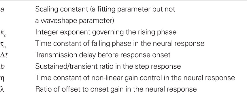
Table 2. Non-linear forward model parameters.
Analytic Framework for the Neural Temporal Response
The starting point for the NDFO modeling is a model of the neural signal, whose first effect in terms of the cascade of BOLD dynamics is to create a metabolic demand G(t) in the neighboring glial cells (see Figure 1). Gamma probability density functions have the analytic form a·tk−1·e−t/τ/Γ(k), where t is the time dimension, a is a scaling parameter, and k and τ are generic waveform parameters. (To equate the area to unity, the function is defined with a = 1/τk), but for the present purposes a is a free optimization parameter.) They may be termed simply “gamma functions” to emphasize their analytic rather than statistical properties. In engineering the same function is known as the n-pole filter function (with n = k), and is used to describe the dynamics of a wide range of processes. For the present application, the temporal gamma function is assumed to have integer powers of k and corresponds to the solution of differential equations with real (non-imaginary) roots. The gamma function has the analytic advantage over many other functions, such as the Gaussian, that it is by definition causal because it has the value of 0 at t = 0, and is defined as 0 for t < 0 (i.e., the full specification is y = kt−1·e−t/τ for t < 0; y = 0 for t < 0). Its shape progresses from highly asymmetric around the peak for small k to approximately Gaussian and symmetric for large k (see Figure 3).
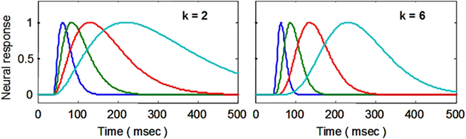
Figure 3. Examples of delayed gamma function step responses with exponents of k = 2 (left) and 6 (right). Successive functions (colors) introduce a wide range of peak latencies for the neural signal estimates (with time constants τ increasing in factors of 2 and a fixed delay Δt of 40 ms).
A key feature of this formalism is that the peak latency is determined by the time constant, τ, and is proportional to the width (at half height) of the response peak, which can be estimated to good accuracy by the methods described in the next section.
Neural Model
A comprehensive model of the BOLD therefore requires an accurate model of the intracellular potential dynamics deriving from the sensory stimulation. Formally, we propose to use the full neural response model jointly specified in Eqs 1 and 2:

where ε is the net source of additive noise and the function is governed by the parameter set.
The neural signal NP(t) in Eq. 1 is the sum of positive and a negative component based on delayed gamma functions convolved with the stimulus waveform:

where 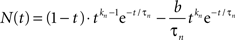
(Note the convention that time series functions are capitalized, impulse response kernels are lower case, and vectors are bold-face.) The neural impulse response expression n(t) is set up so that its convolution with a step function is equivalent to the sum of a pure transient and a pure sustained component. In addition, the expression is specified with an additional transmission delay, Δt, that delays the response relative to the stimulus without affecting its waveshape. Thus, Table 2 defines the parameters in vector p of this equation.
One issue that arises is how to measure the latency Δt of the delayed gamma functions of Figure 3. A simple derivation can show that the peak latency tpeak of these responses is specified by the expression (kτn + Δt). Thus if k and Δt, both of which are well-determined from neurophysiological studies in monkey cortex, are set to means of their Bayesian priors on this basis, the peak latency tpeak is determined from the value of τ, which can be accurately derived from the model optimization.
Metabolic Coupling
Since little is known about the glial dynamics of transmitter recovery, we will pursue two options as to their effects. One option is that the metabolic demand driving the BOLD response derives from the transmitter recovery cycle following the activation by an axonal spike. Since axonal spikes represent only the positive aspect of the intracellular voltage and since 90% of cortical synapses are excitatory (Shank and Aprison, 1979; Wang and Floor, 1994), the signal transmitted from one cortical stage to the next may be treated as a half-wave rectified version of the dynamic neural signal. This prediction is shown as the blue curves in Figure 4Aa (indexed in row/column notation), which is an overlay of the model estimates of the neural responses to stimulus pulses that double in duration from 8 ms to 16 s (eight doublings). For this example, the neural response has balanced excitation and inhibition, so even the prolonged pulses generate only an initial transient response, with the negative lobe at offset being thresholded out by the rectification. (Note that the local metabolic demand, Mi(t), has the same time course in this model as the transmitter recovery from which it derives. The energetic processes required for the recovery to the initial state, however, form an oxygen-based chain of glial metabolic response, G(t), that may have substantially slower time course at one or more stages.)
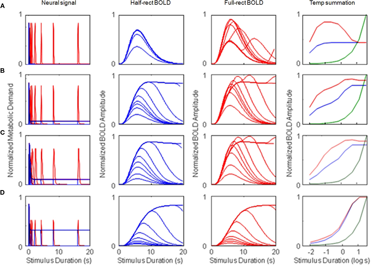
Figure 4. Simulations of four different types of BOLD response for monophasic metabolic demand signals (and a monophasic metabolic response kernel, MRK). The rows represent the results for (A) metabolic demands with a purely transient time course, (B–D) responses with a mixed transient and sustained time course, with the sustained component at respectively 12, 18, and 50% of the amplitude of the transient component (based on different ratios of neural excitation/inhibition). For each type, column (a) shows the assumed metabolic demand, column (b) plots the BOLD responses over duration for the half-wave-rectified model of metabolic demand, column (c) plots the BOLD responses over duration for a fully rectified model, and column (d) plots the duration summation curves for peak amplitude (blue curve: half-rectified model, red curve: fully rectified model, green curve: pure linear summation). Note the use of the logarithmic abscissa in column (d) to focus the analysis on the brief duration regime. The progression of the model BOLD responses with stimulus duration and the form of the summation curves are diagnostic of both the relative weighting between the sustained and transient components of the neural signal and the form of rectification feeding the metabolic demand.
The other option is to consider the instantaneous metabolic demand of both excitatory and inhibitory cells, or both “on” and “off” cells, implying that the signal generating the metabolic demand is a full-wave rectified version of the intracellular voltage. This option is shown as the red curve in Figure 4Aa, whose spikes represent the instantaneous metabolic demand for the offset transient for each of the pulse duration doublings (which were thresholded out in the blue curve).
Having provided relevant variables for the linear and non-linear components of the neural response dynamics, we may now consider the issue of the metabolic coupling of the neural signal to generate the BOLD response. This coupling has been extensively modeled over the past two decades, with the best-known example being the Buxton–Friston balloon model and the most elaborated version being by Sotero and Trujillo-Barreto(2007, 2008). However, these models are not well-validated by empirical human studies (because they contain too many interdependent variables to allow the independent assessment of each separately.
Characteristics of the Model
We may now evaluate the response to these two options for the non-linearity of the metabolic demand through the biophysical chain of the metabolic processes to the measured BOLD signal (Table 1). The first element in this chain is the astrocytes surrounding the neuron, which provide glucose to the neuron and replenish its supply by ATP metabolism fueled by oxygen from neighboring blood vessels. It may be emphasized that the astrocyte metabolic processes are as slow, relative to the intracellular signal dynamics, as are the processes of hemodynamic oxygen supply. The time constant of the astrocyte responses at the cell body is known to be of the order of several seconds (Kelly and van Essen, 1974; Filosa et al., 2004; Metea and Newman, 2006), and it is clear that these slow responses must mediate the hemodynamic component. However, at present too little is known of the dynamics of transmitter recovery and/or the non-linearities in the process to securely assign time constants to the astrocytic component relative to the hemodynamic component of the metabolic coupling. For the present example, we will therefore treat the entire chain from the metabolic demand to the magnetic resonance signal in the traditional fashion, as a unitary linear kernel. As stated above, this kernel is often termed the HRF, but in view of its likely substantial astrocyte contribution, we give it the more general term of the MRK. Our main goal is to estimate the properties of the neural signal processing, and it will be seen that there is sufficient information to provide a rich analysis of these properties, and to account for the empirical non-linearities of the BOLD signal, as long as the metabolic supply chain conforms to the linearity assumption. (As more information becomes available, non-linear aspects of the metabolic coupling may readily be incorporated into the analysis we propose.)
The development of the peak amplitude in the BOLD temporal summation series is shown as the blue summation curve in Figure 4Ad. The critical point of this plot is that the asymptotic corner of this summation curve occurs at 40 ms, which is the value of the time constant assumed for the neural signal in this example. Thus, the form of the BOLD amplitude summation series (Figure 4, column d) provides a direct empirical estimate of the time constant of neural integration down to the millisecond range. There is no limit in principle to the temporal resolution that can be achieved by this methodology since it is estimated from the amplitude variation of the BOLD signal as a function of stimulus duration, not from its temporal aspects.
The reduction in peak amplitude is captured in the red temporal summation curve of Figure 4Ad, showing a reduction by a factor of two for long durations. (The green curve in Figure 4Ad represents the values expected for fully proportional linear summation of the energy in the stimulus pulse; it is an accelerating curve due to the logarithmic abscissa.) The case of the full-rectification model of the metabolic demand is shown in Figure 4Ac. Here the second neural response peak (i.e., that from the stimulus offset) plays a key role in varying the BOLD waveform, which first extends in time and then shows a two-peaked structure with reduced amplitude for long-duration stimuli.
Figure 4Ba shows the half- and fully rectified version of the metabolic demand to the same pulse duration series, where the neural inhibition is now assumed to be reduced in energy by 1.5% relative to the excitation. This small imbalance is magnified by the convolution with the sustained stimulus, and thus it results in a sustained component that is 12% of the amplitude of the initial transient (blue curve in Figure 4Ba) and then into an almost fully sustained set of BOLD response functions (Figure 4Bb, compare to Figure 4Ab). Thus, the form of the BOLD response functions can be strongly diagnostic of even slight variations in the properties of brief neural signals. Moreover, the nature of the metabolic demand function (half- or fully rectified) has a big impact on the form of the BOLD response, determining whether or not an offset peak occurs at the tail of the responses even when they are sustained (Figure 4Bc). Such a peak has been reported in some studies but is not always evident. Thus it remains an empirical question to what extent rectification is representative of BOLD waveforms; intermediate forms of the rectification model are required to capture the empirical properties in detail.
Note that the amplitude series in Figures 4Bb,c show bands of denser packing of the functions, where the amplitude changes were not spaced in proportion to the doublings of stimulus duration. Viewed in terms of the sequence of BOLD waveforms in Figures 4Bb,c, the regions of dense packing form an intermediate “shelf” or partial asymptote in peak amplitude summation plots of Figure 4Bd. It is again evident that the onset of this intermediate shelf in the summation curve corresponds to the integration time of the underlying neural signal, while the second asymptote at higher amplitude corresponds to the ~5 s integration time of the MRK (HRF). Accurate measurement of such summation functions can therefore provide discriminative characteristics that, when interpreted through the non-linear model structure, can provide estimates of both the neural and the metabolic time constants in the neural-to-BOLD signal chain.
This point is emphasized by the response set in row c of Figure 4, which probes the effect of varying the time constant of the neural transient. The key difference from the parameters used in row b of Figure 4, is that the neural time constant was doubled from 50 to 100 ms (and the excitation/inhibition imbalance was also increased to 7% to maintain the same form of offset peak). It is evident that (i) the summation curve (Figure 4Cd) takes a measurably different form, and that (ii) the accuracy of estimation of the neural time constant is limited not by the BOLD time constant but only by the variability of the BOLD amplitude measures. For example, this analysis shows that the neural time constant is estimable to within about 0.1 log units if the BOLD response functions can be measured to an achievable accuracy of about 10%.
The final case of duration summation analyses (Figure 4Dd) shows the NDFO predictions of increasing the excitation/inhibition imbalance of the neural response to 50%, illustrative of a system that is predominantly sustained in nature. Under these conditions, the impact of the initial transient becomes essentially negligible, and the summation curves (Figure 4Dd) become indistinguishable from proportional summation (i.e., they run parallel to the green curve). This manipulation illustrates that the power of the NDFO analysis depends on the neural processing being predominantly transient, and that the properties of the underlying neural mechanisms would not be accessible to this form of analysis in predominantly sustained systems. Luckily, however, the well-established deviation from proportionality for short-duration stimuli implies that the neural system is, in practice, predominantly transient and is therefore amenable to this form of NDFO analysis.
Validation of the Forward Model Analysis
To validate the model framework described in the previous sections in a specific implementation, and to determine the sensitivity of the model parameters to experimental noise sources, we conducted a specific BOLD fMRI experiment.
Methods
Ethics statement
This research was approved by the institutional review board of the University of California, San Francisco, with informed consent obtained for the fMRI study.
Stimulus presentation
The stimuli were spatial arrays of Gabor patches scaled to maximally stimulate retinotopic cortices at all eccentricities. They were presented in durations from a single frame of 16.67 ms duration in factors of 2 to 1.067 s (Figure 5A) in a fully balanced m-sequence design. The durations were presented with full counterbalancing by the m-sequence design. M-sequences are pseudorandom sequences that fully counterbalance the order of stimulus presentation up to a memory length of m-sequential items (Golomb, 1967; Sutter, 1987, 1991; Buracas and Boynton, 2002). They therefore specify the ideal order of presentation of stimuli given that the memory length of the system is known. The m-sequence design is constrained by the fMRI modality, since its analysis is inherently slower than for the ERP. The interstimulus interval was set at 4 s, as we have found that this is an optimal rate for fMRI studies. The typical BOLD response lasts for about 16 s, so this is the length of time over which the response sequence needs to be balanced. Quantitatively, with a sampling time of TR = 2 s and an interstimulus interval of 4 s, we used an m-sequence that balanced all combinations of eight stimuli over a memory duration of 16 s (= 4 samples).
Figure 5. Non-linear dynamic forward model of BOLD responses optimized to a full stimulus duration series. (A) Stimulus time courses for a wide range of stimulus durations. (B) BOLD responses to each stimulus duration (red points, and jackknife error bars), together with the NDFO fit of to the data (blue lines) compared with the fit of a linear model (cyan dashed curves). (C) Estimated neural time course to each stimulus duration (note the 0–1.5 s time scale). White zone is the ±1σ confidence interval for the resultant fit (excluding the transmission delay parameter). (D). Estimated BOLD impulse response at the last stage of the NDFO. (E). Amplitude/duration function for the data (red circles), with the best-fitting prediction from the NDFO (blue curve) compared with the prediction for strict temporal proportionality to stimulus duration (cyan line).
fMRI data collection
Functional MRI scanning was conducted on a Siemens Trio 3 T scanner equipped with eight-channel SENSE parallel imaging capability. In targeting the specific activation sites, it is important to avoid artifactual spread of the activation by partial-voluming across cortex and between blood vessels and cortex on the two sides of a sulcus. Such artifactual spread may account for much of the apparently distributed activation in previous studies with large voxels, and is almost never discussed in relation to studies of the activation patterns for visual processing tasks.
To avoid partial-voluming with the blood vessel overlying the cortex, we make the voxels small enough to lie strictly within the cortical gray matter. For a cortical thickness of 2.5 mm, a sampling analysis shows that the ~33 mm voxels in a typical retinotopy scan have an average of more than half (60%) of their volume outside the cortex, and even across to the other side of a sulcus. (The situation is obviously far worse if the data are averaged to 43 mm effective voxel size. If, however, the voxels are reduced to 23 mm, a continuous sheet of voxels could be found to lie almost entirely within the cortex (an average of 80% isolation of each sample volume).
Our current recording parameters achieve such resolution with an in-plane matrix size of 96 at 23 mm isotropic resolution by using TR = 2 s (with TE = 27 ms, flip angle = 90°), interleaved by staggering the event timings to give an effective temporal resolution of 1 s for the BOLD temporal waveform (see Appendix for details). The 4 cm depth provided sufficient coverage for the posterior occipital lobe in each hemisphere. Activations were analyzed only for voxels lying within the cortical gray matter, as defined by an anatomical segmentation algorithm). The voxels were selected as those lying within the calcarine sulcus, and were therefore restricted to primary visual cortex (V1).
Error bars
To obtain both the individual responses and the standard errors required for the maximum entropy estimation procedure, we employ a novel use of the jackknife procedure specified by Efron and Tibshirani (1993). In brief, to determine the error variance for each repeat in an experiment with i = 1,2,…,n repeats of a given stimulus condition, n − 1 jackknife estimates for each of the event types in the design matrix are derived by re-running the analysis with each repeat of the chosen event removed in succession from the design matrix.
Under the jackknife procedure, the standard error of the mean (SEM) for each datum point of the response matrix X(k,t) for each event type k at each time point t is calculated from the ith-deleted pseudovalues according to
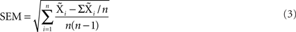
where 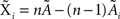 , with
  and
and  being the average and the ith-deleted average vectors, respectively.
Results
Bold Responses
To validate our conceptual breakthrough for the estimation of neural response dynamics from BOLD response measurements we performed a computational analysis of the implications of the BOLD fMRI data collected on a typical human subject with corrected to normal vision, a temporal modulation sensitivity function within normal limits, typical event-related potentials to contrast reversal (onset latency of 52 ms and N1 latency of 115 ms) and a typical BOLD response time course as evident from Figure 5 and a number of previous retinotopic and localizer scans. The analysis was conducted in a full-range temporal summation paradigm (Figure 5A) and provides not only the estimated neural response waveform but confidence limits on the waveform parameters that are sufficiently narrow to indicate that the results are within the expected range for early cortical response dynamics.
The responses from primary visual cortex (~250 voxels) for a 1-h session from a typical subject are shown in Figure 5B. They show a progressive growth in amplitude with stimulus duration from the shortest to the longest, but note that the amplitudes do not increase by a factor of two (the linear GLM prediction; cyan dashed curves in Figure 5B) as duration is increased. We therefore need a non-linear model to understand the processing mechanism for these effects.
The data have thus been fit through our NDFO procedure of a linear convolution of the stimuli from durations from 16.67 ms to 1.067 s in factors of 2 (Figure 5A) with each neural component kernel to generate the neural signals at each duration (Figure 5C), a non-linear coupling to generate the component metabolic demands, a linear summation over the component demands to generate the net metabolic demand, and a linear convolution with a MRK (Figure 5D) to generate the ultimate BOLD signal prediction (Figure 5B). Figure 5E is a comparison of the amplitudes of the fitted model waveforms with those of the data, as analyzed in Section “Discussion.” Optimization of the BOLD prediction (blue curves in Figure 5B) to the data determines the temporal features of the requisite neural signals making up each waveform, allowing us to specify the predominant time constants for the underlying neural signals. These features are defined by the following model population parameters for the net neural signal throughout each studied cortical region: transmission delay, gamma exponent, recovery time constant, sustained/transient ratio, sustained decay, and off/on ratio (six waveform parameters). The amplitude, transient integration time, and sustained/transient ratio are specified to worthwhile precision (see Appendix). The off/on ratio parameter controlling the relative amplitude of the off-responses is not well-constrained for the duration-range used in this data set (Figure 5), but we note that this parameter could also be brought under tighter control by adding stimuli of longer duration (e.g., 8 s). This approach should readily provide tight constraints on the off/on ratio because the BOLD activity corresponding to the off-responses is pushed to a time period that is essentially independent of that for the on response. This kind of approach to the off transient had been taken successfully by Fox et al. (2005) and Lingnau et al. (2009), for example.
Discussion
Our novel analysis of the neural signal underlying the BOLD response waveforms to a full temporal stimulus series constitutes a form of “temporal microscope” for the neural signals in the cortex generating the recorded BOLD waveforms. Thus, this study illustrates how the neural waveform parameters can be estimated from the temporal summation series to their native temporal resolution. The estimated neural waveform for the present dataset in Figure 5C has a strong brief transient with a width at half height of 55 ms, followed by a sustained response of about 1/10th of the peak transient response and a reduced, but rectified, offset response at the end of each stimulus. In each respect, these response properties match the corresponding neural response properties recorded in the cortex of other species. A useful survey of the dynamics of the unitary intracellular responses to single synaptic action potentials is provided by Thomson and Lamy (2007). They tabulate data from a large number of studies of the excitatory post-synaptic potential (EPSP) time course, 54 of which have usable data on the exponential time constant of decay. These are analyzed in Section “Appendix” to show that the typical EPSP time constant has a standard deviation of ±20 ms. This kind of analysis can provide the Bayesian constraints on the modeling, although we note that the typical afferent volley has a temporal spread of about ±20 ms that must be convolved with the EPSP time constant to obtain an estimate of the metabolic demand generated by the typical synaptic activation. Thus, the net time course of the neural transients is expected to have a standard deviation of the order of 28 ms, or a full width at half height of ~50 ms. We are not aware of comparable meta-analysis for monkey cortical responses, but this value is clearly in line with the published examples of V1 transients from this species (such as those of Hegdé and van Essen, 2004).
It must be emphasized that the transient time-constant analysis relies on the deviation from the linear model of proportional responses (indicated by the cyan line in amplitude plot of Figure 5E). Such deviations can be accurately determined because they are based on the integrated response amplitude at short durations. The accuracy of the model fit does not depend on this linearity assumption, but could be fit equally well to a non-linear temporal integration behavior if that behavior were specifiable for typical neural populations. To our knowledge, however, neural signals exhibit linear temporal integration at this time scale (e.g., Koch, 2005), and the primary non-linearity is the inability of the spike rate to fall below 0, coupled with the presence of both ON and OFF type neurons, which result in a fully rectified spike-rate response for the typical population of a cortical voxel. Just how the spike rate is coupled to the metabolic demand, in terms of its rectification behavior, has not yet been determined, which is why we provide an example analysis in Figure 4 of how the determination of one form of non-linearity can be made in the framework of the present analysis.
Similarly, as knowledge evolves, more complex models of the neural/metabolic coupling and the hemodynamic response could be easily incorporated in our model. These all represent Bayesian information that, if well-established, can be used to refine the model structure and enhance the fitting process when available. However, our understanding of the literature is that (a) the first-order specification of the neural/BOLD coupling is well approximated by a linear response kernel, and (b) that estimates of the second-order effects are contaminated by the assumption that they are purely hemodynamic, and have not taken into account potential and actual non-linearities in the neural signals at the time scale of the BOLD signal. Thus, despite the best efforts of the proponents of elaborated hemodynamic modeling, there is no secure information about the non-linearities of this process for the human brain in vivo. Consequently, we have tried to redress the balance by considering the effects plausible non-linearities in the neural population responses to standard types of stimulus presentation. For clarity in this enterprise, we have assumed that the metabolic response is both linear and monophasic, illustrating a variety of BOLD response properties that could arise from such neural non-linearities. We are not claiming to have proven that these BOLD properties are entirely determined at the neural level (which would be a vast enterprise, far beyond the scope of one paper), but that claims that they are purely properties of the vascular hemodynamics per se are suspect until they are replicated in paradigms that remove the neural component of the system [such as stimulation of the hemodynamic response by direct infusion of nitric oxide (NO) in the vicinity of the blood vessels. This experiment has apparently not been attempted, although Burke and Bührle (2006) showed that suppression of the NO with application of the NO synthase inhibitor 7-nitroindazole completely abolished the BOLD response while only marginally affecting the local field potentials, establishing the role of NO in neurovascular coupling.]
In particular, the non-linearity of the transient responses at the offset of the neural response could be positive (rectifying) rather than negative (linear), and could in either case show reduced amplitude relative to the onset response (adaptive gain control). In this example of the NDFO analysis, the offset responses are much smaller than the positive responses at stimulus onset. This analysis demonstrates that estimation of the neural response dynamics for each stimulus type is therefore not a Herculean task requiring extreme levels of signal/noise ratio, but is well within the capability of one session of normal fMRI methodology using, however, the appropriate combination of experimental design and theoretical analysis.
We note that a technique with a philosophy similar to the present approach has been successfully applied to the estimation of net spatial receptive field structure of small cortical regions by Dumoulin and Wandell (2008), although they used a linear rather than the full non-linear model of the sequence of processes. Their spatial estimates were based on a model of the temporal signal to be expected as a stimulus swept across each defined point on the retina. Like us, they take the temporal stimulus waveform, convolve it with a spatiotemporal model of the response of the underlying neural population, and then with a model of the MRK (HRF) to provide a forward model of the temporal BOLD response that is optimized to the measured BOLD response at each cortical location. Our approach takes the temporal analysis several steps further toward biological plausibility, and focuses on the temporal rather than spatial aspect of the neural population response, but the general philosophy of analyzing interesting parameters of the neural response through a forward model of the BOLD response is a similar one.
Conclusion
The conceptualizations and techniques introduced in this paper provide an analytic capability to resolving the timing and neural signal estimation underlying the BOLD waveforms recorded throughout the cortex. Any such attempt must be based on a model of the known neural dynamics of the neural populations underlying the BOLD metabolic signal generation, which may be progressively refined as more information becomes available about both neural response characteristics and the metabolic cascade. Given adequate signal/noise ratio, the present analysis shows that it is possible to develop approaches that overcome the temporal limitations of BOLD signal and are able to reveal the relevant properties of the underlying neural signals down to their native temporal resolution. In combination, these approaches represent a notable advance in the capabilities of the fMRI technology, providing a direct linkage between the live assessment of the functioning brain and the direct neurophysiological recordings in other species.
Conflict of Interest Statement
The authors declare that the research was conducted in the absence of any commercial or financial relationships that could be construed as a potential conflict of interest.
Acknowledgments
Supported by NSF grant # SLC 6814855 to Christopher W. Tyler and NSF grant # SBE/SLC 0846430 to Lora T. Likova.
Footnote
- ^The term “kernel” is preferred because it is conceptualized as the theoretical response to an imaginary stimulus of infinitely short duration and unit area, termed a “Dirac pulse.”
References
Aguirre, G. K., Zarahn, E., and D’Esposito, M. (1998). The variability of human BOLD hemodynamic responses. Neuroimage 8, 360–369.
Azouz, R., and Gray, C. M. (1999). Cellular mechanisms contributing to response variability of cortical neurons in vivo. J. Neurosci. 19, 2209–2223.
Bandettini, P. A., and Ungerleider, L. G. (2001). From neuron to BOLD: new connections. Nat. Neurosci. 4, 864–866.
Bandettini, P. A., Birn, R. M., Kelley, D., and Saad, Z. S. (2002). Dynamic nonlinearities in BOLD contrast: neuronal or hemodynamic? Elsevier Excerpta Medica Int. Congr. Ser. 1235, 73–85.
Barth, M., and Norris, D. G. (2007). Very high-resolution three-dimensional functional MRI of the human visual cortex with elimination of large venous vessels. NMR Biomed. 20, 477–484. doi: 10.1002/nbm.1158
Bellgowan, P. S., Saad, Z. S., and Bandettini, P. A. (2003). Understanding neural system dynamics through task modulation and measurement of functional MRI amplitude, latency, and width. Proc. Natl. Acad. Sci. U.S.A. 10, 1415–1419.
Bevington, P. R., and Robinson, D. K. (2003). Data Reduction and Error Analysis for the Physical Sciences. New York, NY: McGraw-Hill.
Birn, R. M., Saad, Z. S., and Bandettini, P. A. (2001). Spatial heterogeneity of the nonlinear dynamics in the FMRI BOLD response. Neuroimage 14, 817–826.
Boynton, G. M., Engel, S. A., Glover, G. H., and Heeger, D. J. (1996). Linear systems analysis of functional magnetic resonance imaging in human V1. J. Neurosci. 16, 4207–4221.
Buracas, G. T., and Boynton, G. M. (2002). Efficient design of event-related fMRI experiments using m-sequences. Neuroimage 16, 801–813.
Burke, M., and Bührle, C. (2006). BOLD response during uncoupling of neuronal activity and CBF. Neuroimage 32, 1–8.
Buxton, R. B., Uludağ, K., Dubowitz, D. J., and Liu, T. T. (2004). Modeling the hemodynamic response to brain activation. Neuroimage 23 (Suppl 1), S220–S233.
Carandini, M., and Ferster, D. (1997). A tonic hyperpolarization underlying contrast adaptation in cat visual cortex. Science 276, 949–952.
Carandini, M., and Ferster, D. (2000). Membrane potential and firing rate in cat primary visual cortex. J. Neurosci. 20, 470–484.
Celebi, S., and Principe, J. C. (1995). Parametric least squares approximation using gamma bases. IEEE Trans. Signal Process. 43, 781–784.
Chatton, J. Y., Pellerin, L., and Magistretti, P. J. (2003). GABA uptake into astrocytes is not associated with significant metabolic cost: implications for brain imaging of inhibitory transmission. Proc. Natl. Acad. Sci. U.S.A. 100, 12456–12461.
d’Avossa, G., Shulman, G. L., and Corbetta, M. (2003). Identification of cerebral networks by classification of the shape of BOLD responses. J. Neurophysiol. 90, 360–371.
De Vries, B., and Principe, J. C. (1992). The gamma model: a new neural model for temporal processing. Neural Netw. 5, 565–576.
de Zwart, J. A., Silva, A. C., van Gelderen, P., Kellman, P., Fukunaga, M., Chu, R., Koretsky, A. P., Frank, J. A., and Duyn, J. H. (2005). Temporal dynamics of the BOLD fMRI impulse response. Neuroimage 24, 667–677.
Dumoulin, S. O., and Wandell, B. A. (2008). Population receptive field estimates in human visual cortex. Neuroimage 39, 647–660.
Efron, B., and Tibshirani, R. J. (1993). An Introduction to the Bootstrap. New York: Chapman & Hall.
Farwell, V. T., and Prentice, R. L. (1977). A study of distributional shape in life testing. Technometrics 19, 69–75.
Filosa, J. A., Bonev, A. D., and Nelson, M. T. (2004). Calcium dynamics in cortical astrocytes and arterioles during neurovascular coupling. Circ. Res. 95, 73–81.
Fox, M. D., Snyder, A. Z., Barch, D. M., Gusnard, D. A., and Raichle, M. E. (2005). Transient BOLD responses at block transitions. Neuroimage 28, 956–966.
Friston, K. J., Fletcher, P., Josephs, O., Holmes, A., Rugg, M. D., and Turner, R. (1998). Event-related fMRI: characterizing differential responses. Neuroimage 7, 30–40.
Friston, K. J., Mechelli, A., Turner, R., and Price, C. J. (2000). Nonlinear responses in fMRI: the Balloon model, Volterra kernels, and other hemodynamics. Neuroimage 12, 466–477.
Glover, G. (1999). Deconvolution of impulse response in event-related BOLD fMRI. Neuroimage 9, 416–429.
Grotz, T., Zahneisen, B., Ella, A., Zaitsev, M., and Hennig, J. (2009). Fast functional brain imaging using constrained reconstruction based on regularization using arbitrary projections. Magn. Reson. Med. 62, 394–405.
Handwerker, D. A., Ollinger, J. M., and D’Esposito, M. (2004). Variation of BOLD hemodynamic responses across subjects and brain regions and their effects on statistical analyses. Neuroimage 21, 1639–1651.
Harel, N., Lin, J., Moeller, S., Ugurbil, K., and Yacoub, E. (2006). Combined imaging-histological study of cortical laminar specificity of fMRI signals. Neuroimage 29, 879–887.
Hegdé, J., and van Essen, D. C. (2004). Temporal dynamics of shape analysis in macaque visual area V2. J. Neurophysiol. 92, 3030–3042.
Hegdé, J., and Van Essen, D. C. (2006). Temporal dynamics of 2D and 3D shape representation in macaque visual area V4. Vis. Neurosci. 23, 749–763.
Heinzer, S., Krucker, T., Stampanoni, M., Abela, R., Meyer, E. P., Schuler, A., Schneider, P., and Müller, R. (2006). Hierarchical microimaging for multiscale analysis of large vascular networks. Neuroimage 32, 626–636.
Henson, R. N., Price, C. J., Rugg, M. D., Turner, R., and Friston, K. J. (2002). Detecting latency differences in event-related BOLD responses: application to words versus nonwords and initial versus repeated face presentations. Neuroimage 15, 83–97.
Hoge, R. D., Franceschini, M. A., Covolan, R. J., Huppert, T., Mandeville, J. B., and Boas, D. A. (2005). Simultaneous recording of task-induced changes in blood oxygenation, volume, and flow using diffuse optical imaging and arterial spin-labeling MRI. Neuroimage 25, 701–707.
Kelly, J. P., and van Essen, D. C. (1974). Cell structure and function in the visual cortex of the cat. J. Physiol. 238, 515–547.
Koch, C. (2005). Biophysics of Computation: Information Processing in Single Neurons. New York: Oxford University Press.
Likova, L. T., and Tyler, C. W. (2007). Instantaneous stimulus paradigm: cortical network and dynamics of figure-ground organization. Proc. SPIE 6492, 64921E.
Lin, F. H., Witzel, T., Mandeville, J. B., Polimeni, J. R., Zeffiro, T. A., Greve, D. N., Wiggins, G., Wald, L. L., and Belliveau, J. W. (2008). Event-related single-shot volumetric functional magnetic resonance inverse imaging of visual processing. Neuroimage 42, 230–247.
Lingnau, A., Ashida, H., Wall, M. B., and Smith, A. T. (2009). Speed encoding in human visual cortex revealed by fMRI adaptation. J. Vision 9, 3.1–14.
Logothetis, N. K. (2002). The neural basis of the BOLD fMRI signal. Philos. Trans. R. Soc. Lond. B Biol. Sci. 357, 1003–1037.
Logothetis, N. K. (2003). The underpinnings of the BOLD functional magnetic resonance imaging signal. J. Neurosci. 23, 3963–3971.
Logothetis, N. K., and Wandell, B. A. (2004). Interpreting the BOLD signal. Annu. Rev. Physiol. 66, 735–769.
Magistretti, P. J. (2009). Role of glutamate in neuron-glia metabolic coupling. Am. J. Clin. Nutr. 90, 875S–880S.
Magistretti, P. J., and Pellerin, L. (1999). Cellular mechanisms of brain energy metabolism and their relevance to functional brain imaging. Philos. Trans. R. Soc. Lond. B Biol. Sci. 354, 1155–1163.
Martindale, J., Mayhew, J., Berwick, J., Jones, M., Martin, C., Johnston, D., Redgrave, P., and Zheng, Y. (2003). The hemodynamic impulse response to a single neural event. J. Cereb. Blood Flow Metab. 23, 546–555.
Mechelli, A., Price, C. J., and Friston, K. J. (2001). Nonlinear coupling between evoked rCBF and BOLD signals: a simulation study of hemodynamic responses. Neuroimage 14, 862–872.
Menon, R. S., Luknowsky, D. C., and Gati, J. S. (1998). Mental chronometry using latency-resolved functional MRI. Proc. Natl. Acad. Sci. U.S.A. 95, 10902–10907.
Metea, M. R., and Newman, E. A. (2006). Glial cells dilate and constrict blood vessels: a mechanism of neurovascular coupling. J. Neurosci. 26, 2862–2870.
Meyer, E. P., Ulmann-Schuler, A., Staufenbiel, M., and Krucker, T. (2008). Altered morphology and 3D architecture of brain vasculature in a mouse model for Alzheimer’s disease. Proc. Natl. Acad. Sci. U.S.A. 105, 3587–3592.
Nowak, L. G., and Bullier, J. (1997). “The timing of information transfer in the visual system,” in Cerebral Cortex and Extrastriate Cortex in Primates, Vol. 12, eds K. Rockland, J. Kaas, and A. Peters (New York, NY: Plenum Press), 205–241.
Shank, R., and Aprison, M. (1979). “Biochemical aspects of the neurotransmitter function of glutamate,” in Glutamic Acid: Advances in Biochemistry and Physiology, eds L. J. Jr. Filer, S. Garattini, M. R. Kare, W. A. Reynolds, and R. J. Wurtman (New York, NY: Raven), 139–150.
Shao, X. M. (1997). Parametric survival analysis for gating kinetics of single potassium channels. Brain Res. 770, 96–104.
Shmuel, A., Augath, M., Oeltermann, A., and Logothetis, N. K. (2006). Negative functional MRI response correlates with decreases in neuronal activity in monkey visual area V1. Nat. Neurosci. 9, 569–577.
Sotero, R. C., and Trujillo-Barreto, N. J. (2007). Modelling the role of excitatory and inhibitory neuronal activity in the generation of the BOLD signal. Neuroimage 35, 149–165.
Sotero, R. C., and Trujillo-Barreto, N. J. (2008). Biophysical model for integrating neuronal activity, EEG, fMRI and metabolism. Neuroimage 39, 290–309.
Sun, F. T., Miller, L. M., and D’Esposito, M. (2005). Measuring temporal dynamics of functional networks using phase spectrum of fMRI data. Neuroimage 28, 227–237.
Sutter, E. E. (1987). “A practical nonstochastic approach to nonlinear time-domain analysis,” in Advanced Methods in Physiological System Modelling, Vol. 1, ed. V. Z. Marmarelis (Los Angeles: University of Southern California Press), 303–315.
Sutter, E. E. (1991). The fast m-transform: a fast computation of cross-correlation with binary m-sequences. SIAM J. Comput. 20, 686–694.
Thomson, A. M., and Lamy, C. (2007). Functional maps of neocortical local circuitry. Front. Neurosci. 1:1, 19–42.
Thompson, J. K., Peterson, M. R., and Freeman, R. D. (2003). Single-neuron activity and tissue oxygenation in the cerebral cortex. Science 299, 1070–1072.
Thompson, J. K., Peterson, M. R., and Freeman, R. D. (2004). High-resolution neurometabolic coupling revealed by focal activation of visual neurons. Nat. Neurosci. 7, 919–920.
Thompson, J. K., Peterson, M. R., and Freeman, R. D. (2005). Separate spatial scales determine neural activity-dependent changes in tissue oxygen within central visual pathways. J. Neurosci. 25, 9046–9058.
Keywords: fMRI, cortical processing, human, visual, neural dynamics, blood oxygen level dependent
Citation: Tyler CW and Likova LT (2011). Estimating neural signal dynamics in the human brain. Front. Syst. Neurosci. 5:33. doi: 10.3389/fnsys.2011.00033
Received: 10 June 2010;
Accepted: 11 May 2011;
Published online: 06 June 2011.
Edited by:
Robert Shapley, New York University, USAReviewed by:
Stephen A. Engel, University of Minnesota, USACheryl Olman, University of Minnesota, USA
Copyright: © 2011 Tyler and Likova. This is an open-access article subject to a non-exclusive license between the authors and Frontiers Media SA, which permits use, distribution and reproduction in other forums, provided the original authors and source are credited and other Frontiers conditions are complied with.
*Correspondence: Christopher W. Tyler, The Smith-Kettlewell Eye Research Institute, 2318 Fillmore Street, San Francisco, CA, USA. e-mail:Y3d0QHNraS5vcmc=