Analysis of Primary Care Computerized Medical Records (CMR) Data With Deep Autoencoders (DAE)

1. Introduction

Computerized Medical Records (CMR)s (also known as electronic health records or electronic medical records) are a digital storage of health information for individuals. These digital records are the standard way for medical professionals, such as General Practitioners (GPs) to record primary healthcare data for patients. Identifying patterns in primary care data is vital in forecasting responses or policies to healthcare issues; for example, early warning for potential epidemics allows healthcare organization to take preventative measures such as vaccination or quarantine. Data quality and veracity assessments are vital for decision making [1] as they can have implications in not only health, but can also have social, economic and political impacts. In many cases, primary care records contain indicators for the health at a population level that are nationally representative [2] and analysis of these data can lead to improvements for disease incidence estimates in surveillance systems [3]. The Royal College of General Practitioners (RCGP) Research and Surveillance Centre (RSC) [4, 5] collects primary care data for a number of respiratory infections and other conditions, focusing on influenza. The network is used annually by the UKs Chief Medical Officer to know when influenza is circulating and which age groups are most at risk [5]. For instance, the RCGP RSC data showed that in 1989–1990 children were most affected by influenza, and in 2000 older people were at risk of infection [6]. The RSC was also pivotal in identifying and monitoring the 2009-2010 swine flu pandemic [7]. However, methods for utilizing large primary care data are limited and inferring meaning from these data is challenging [8]. Despite these difficulties, the potential for identifying trends in CMR data are significant. Predictive algorithms may help tackle higher mortality observed in winter months [9], or forecast unexpected spikes in mortality rates due to the spread of influenza [10].

Methods for pre-processing synthetic data to reduce complexity prior to clustering have been demonstrated as an effective way to analyse CMR type data [11]. Low dimensional representations of complex systems can provide great insights into patterns or behaviors that are otherwise difficult or impossible to obtain directly [12–14]. Multivariate and machine learning methods have emerged as powerful tools in data analysis. Specifically, clustering methods have shown potential in analysis of medical records [15], however, they rely on complete, non-redundant and homogenous data, where CMR data are typically heterogeneous, incomplete, and contain redundancies and uninformative fields [11].

Over the last decade, the power of deep learning has shown its potential in a number of areas to extract patterns from complex data without bespoke pre-processing or normalizations [16–18]. Deep learning has very recently been used to aid palliative care by improving prognosis estimates based on healthcare data [19]. The generality of these methods is attractive in studying complex and dynamic problems such as CMR data, where the fields in the data vary significantly in format, complexity, redundancy, noise, and size for differing requirements. The data fields extracted from a medical record database will vary drastically depending on the research question and corresponding extraction query. Deep learning methods offer a powerful and practice suite of tools for analysis of CMR data.

In this work we propose a deep learning method for visualizing and analysing CMR data to identify low dimensional patterns in the data, such as manifolds or clusters, that would not otherwise be obtainable in the high dimensional space. Our proposed workflow could be used to aid healthcare practitioners in decision making based on the individual or population based data. In the following sections we describe the data and methods, and discuss the results of our analysis. All data used in this work is fully anonymised and complies with the RCGP RSC protocols and ethics.

2. Materials and Methods

Deep learning algorithms have been applied to a diverse range of problems in a number of areas of research. In particular, deep neural networks have emerged as popular tools for several tasks such as segmentation and classification. A significant limitation to their use has been the requirement for a large amount of labeled data for training networks for such tasks. Additionally, for applications in clinical settings, the lack of transparency in the decision making is extremely problematic and may limit the uptake in many other areas.

Hinton and Salakhutdinov introduced the use of the autoencoder for unsupervised dimensionality reduction [17], sidestepping the requirement for explicitly labeled data by training a network to first encode the input data, then decode this back to the input data. In this framework, the network is trained to learn an encoding of the data that can be decoded back to the input data, which does not require explicit labels. Additionally, these networks can be trained such that we obtain a fixed and deterministic transformation between the input and encoded data, enabling several advantages such as maintaining a common encoded space for training and unseen data. This allows the time and memory efficient application of these algorithms to large datasets [18], as well as identifying the features that are driving patterns in the data. We utilize these features of the autoencoder to perform non-linear unsupervised dimensionality reduction of computerized medical records (CMR) enabling visualization, unsupervised data exploration, and pattern recognition that is both deterministic and traceable. In the following subsections we outline the data handling, processing and analysis used in this work.

2.1. Computerized Medical Records

CMRs are a collection of attributes from anonymised patients, containing a mix of data types (numeric, text, etc.). The data has been collected and stored by the RCGP RSC [4, 5]. All data are from English General Practices (GPs) and consist of 2.4 million records from > 230 GPs that is representative of the national population [5]. CMR data are uploaded to the RSC twice per week with each upload containing data from a 6 week period, with overlapping uploads to account for post-acquisition data correction by the medical professional. In this study, we analyse attributes extracted from one of these uploads covering a 6 week period in 2016 for 11,000 medical records, each with nine attributes relating to the patient and condition. Specifically, these are: the patients age and gender, the anonymised ID for the GP sending the data to the SRC, the date of the record, the Clinical System for the record, the Read Term (recorded condition), Read Code (standardized coding for the condition, see [5] for further details), Coding System (the standards for the Read Code), and the Episode which records the status of the condition. The Episode type records whether the condition is new (N), ongoing (O) or first (F), though can also be missing (blank). A large proportion of the 11,000 CMR data (1,067 records) have missing Episode type and cannot be used for routine analysis and reporting. As the most reliable way of differentiating incident from prevalent cases is through the clinician assigning Episode type to the patient's CMR [20] this represents a significant amount of unusable data. An ability to uncover patterns in the data may be useful in identifying sources and commonalities in missing Episode type, which may inform methods for correcting or predicting these errors. Furthermore, looking for patterns or manifolds in the data may reveal other interesting features in the data that are not observable in the original high dimensional space.

The information was extracted from the CMR database RCGP RSC secure servers from the anonymised NHS records data using secure onsite SQL database. Only the necessary fields pre-defined for the study where extracted in line with NHS Digital's Data Security and Privacy (DSP) governance process. The resulting dataset is in a delimited text ASCII text file where columns represent an attribute value and rows correspond to different instances of a record. Each attribute has a column heading and each instance in the dataset is an individual medical record, and thus the data set may contain multiple records from the same patient. The data used in this work, and other datasets, can be requested from the RSC via https://www.rcgp.org.uk/clinical-and-research/our-programmes/research-and-surveillance-centre.aspx.

2.2. Data Pre-processing

The use of heterogeneous data in reduction methods requires some pre-processing [11]. Prior to our reduction method we pre-process the data in order to account for the mixed data formats in the CMR. In our method, we initially convert the mixed format data, containing numerical, date, structured text, unstructured text, and categorical data, into solely numerical values so that all attributes can be processed together to identify patterns between variables. Each instance in the dataset is processed as follows. All numerical fields are converted to doubles. Text data (categorical, structured and unstructured) are converted to unsigned 32-bit integers using the conversion listed in Figure 1 for each character in a string. For text data where instances in the CMR differ in length, first the longest entry in the dataset is identified and all other instances are padded with whitespace characters at the end of the string to this length. Encoding the text data in this way and using an autoencoder provides robustness against errors in the entries such as spelling mistakes or differing orders of words. For date variables, the attributes are read in as text strings in order to account for differing formats across datasets, and converted to the ISO 8601 format yyyy-mm-dd. These variables are then separated into three numerical values corresponding to the year, month, and day of the records to account for any regular patterns such as seasonal variation. After all of the attributes have been converted in to numerical data as described above, the values for an instance in the CMR is concatenated together to a single numerical vector of length M. This is performed for all N instances in the data yielding numerical matrix with dimensions N × M. Specifically for the data used in this work, we obtain a matrix of 11,000 instances each with 93 dimensions. Processing the CMR data in this way ensures the mixed type input data is returned as a numeric matrix of all attributes, that is compatible with a suite of mathematical operations. In particular, we require this format for the CMR in order to use a deep autoencoder which is able to identify patterns in complex, nonlinear and high dimensional data in an unsupervised manner that is computationally efficient. In the next section we outline the details of the network and algorithms used in this work.

FIGURE 1

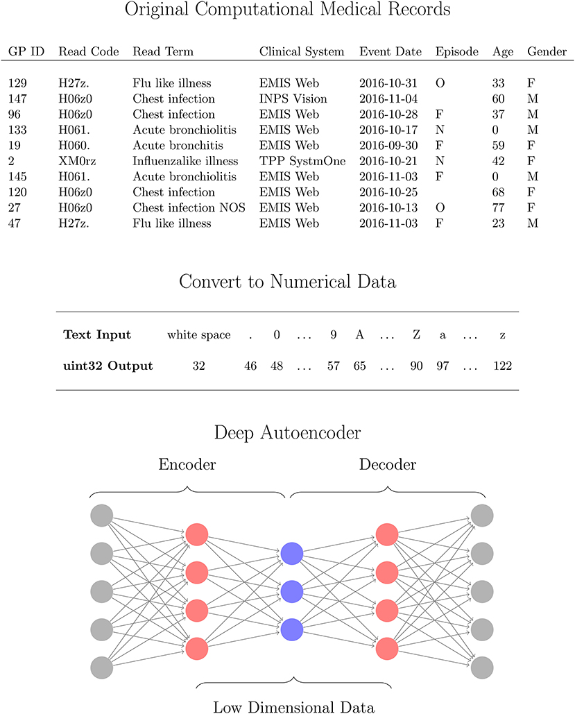
Figure 1. Workflow for analysing computational medical records (CMR) with a deep autoencoder (DAE). The high dimensional CMR data (Top) is converted to Numerical data (Middle) for all attributes using 32uint conversion (MATLAB, 2016a) which are then used as inputs for the DAE (Bottom). The DAE is trained to learn a low dimensional representation (blue neurons) of the converted CMR data (gray neurons) via several hidden layers (red neurons) in an unsupervised manner.

2.3. Deep Autoencoder

An autoencoder is a special class of neural network that is structurally symmetric and is designed to first encode the input data and then decode it back to the input data. This feature enables the autoencoder to be trained in an unsupervised manner as the network learns an encoded representation of the data that can be decoded back to the input data. We implicitly have labels for our data rather than requiring a class label as in typical deep learning problems. Encoding the data refers to an operation that transforms the data into a different space, typically with a lower dimensionality, and decoding refers to a reverse transformation back to the original space. Thus the network takes the N × M input matrix x and encodes it to z, an N × K matrix where typically K < M, then decodes z back to a N × M matrix x′. The performance of the network can be evaluated by comparing the matrix elements in the output of the network with those of the input by calculating the mean squared error ϵ for N training examples

$\begin{array}{ll}ϵ=\frac{1}{N}{\displaystyle \sum _j^N}{ϵ}_j=\frac{1}{N}{\displaystyle \sum _j^N}{\displaystyle \sum _i^M}{(x_{ji}-x_{ji}^{\prime })}^2.& (1)\end{array}$

The encoded data z is obtained through an activation function σ and similarly decoded using the function σ′,

$\begin{array}{ll}z=\sigma \left(Wx+b\right);x^{\prime }={\sigma }^{\prime }\left(W^{\prime }z+b^{\prime }\right);& (2)\end{array}$

The elements of W, W′, b and b′ can be obtained by training the network using gradient descent, hence with Equations (1) and (2) we can train the network in an unsupervised manner. Here we use the scaled conjugate gradient algorithm for our gradient descent [21]. There are a range of activations that can be chosen for σ and σ′, which are often of the same form to provide symmetry in the network and an output that is comparable to the input. Activation functions such as ReLU, σ(z) = max(0, z), are popular in convolutional neural networks due to their success in image analysis problems [16]. Sigmoid activation functions, σ(z) = (1 + e^−z)⁻¹, have also been shown to be useful in reduction and visualization of complex and high dimensional data [22], and identification of low dimensional patterns in the data for segmentation and classification tasks [16, 18]. Here we compare both ReLU and sigmoid activation functions for reduction of the CMR data. The ability to identify nonlinear patterns give DAEs an advantage over linear methods such as PCA [23].

As the autoencoder encodes and decodes the input data, one can stack networks together to form a deep autoencoder of several encoding and decoding layers. This provides a computationally efficient way to train deep networks for high dimensional data by performing layer-wise training. This is achieved by passing the encoded data from one layer as input in to the next layer which is then trained in the same way. Stacking these layers together produces a deep network that consists of several encoding layers followed by several decoding layers. Typically, each layer encodes the input data into a lower dimensional space to identify manifolds in the system. We use a deep autoencoder consisting of four encoding layers that reduce the dimensionality of the input data from 93 to 50, 20, 10, and 3 dimensions before decoding this back to the dimensionality of the input data as illustrated in Figure 1. Reduction of high dimensional data to two or three dimensions is common for visualization of these data as they can reveal patterns in the low dimensional space. The data form these manifolds or clusters based on patterns in the data such as structure in images [24], text documents [16, 17], hyperspectral data [25], transcriptomics [26], gene [27], and cell expression [28]. We construct our deep autoencoder such that the lowest dimensionality of the encoded data consists of three deep features, so that it can be visualized as a scatter plot. The number of hidden layers, and neurons within each, were selected from initial configuration optimization. For the data in this work, increasing the number of layers did not provide notable improvements to the network performance whilst increasing training and computation time. It was also observed that the number of neurons in each layer had little effect compared to regularization.

We employ an L₂ weight regularization, also known as Tikhonov regularization, to reduce the complexity of W and improve the conditioning of the problem. This form of regularization is known to prevent overfitting in training [29–31], by restricting the magnitude of values in W. This is calculated for L hidden layers, M inputs and K outputs,

$\begin{array}{ll}{\Omega }_w=\frac{1}{2}{\displaystyle \sum _l^L{\left(W^{(l)}\right)}^2}=\frac{1}{2}{\displaystyle \sum _l^L{\displaystyle \sum _m^M{\displaystyle \sum _k^K{\left(w_{mk}^{(l)}\right)}^2}}}.& (3)\end{array}$

The average output of neuron k is defined as

$\begin{array}{ll}{\widehat{\rho }}_k=\frac{1}{N}{\displaystyle \sum _{j=1}^N}{z}_{jk},& (4)\end{array}$

and measure how responsive the network is to features in the input data. A low average activation indicates that the neuron is only responding to very specific features, whereas higher values indicate that the neuron is not distinguishing between instances in the data. In order to constrain this, we include a sparsity regularization for the average output of each neuron in the network. This will constrain the output from each neuron to approximate a specified level, enabling them to respond to particular features while also learning general features, and thus leading to an encoding that distinguishes sub-types in the data based on their attributes. The sparsity is constrained using the Kullback-Leibler (KL) divergence between the desired level of activation, ρ, and the average output $\widehat{\rho }$

$\begin{array}{ll}{\Omega }_s={\displaystyle \sum _{k=1}^K}\rho log\left(\frac{\rho }{{\widehat{\rho }}_k}\right)+\left(1-\rho \right)log\left(\frac{1-\rho }{1-{\widehat{\rho }}_k}\right).& (5)\end{array}$

The first term of Equation (5) is the typical KL divergence, and the second term is included to introduce non-negativity in the metric and control the level of asymmetry in the function via $\widehat{\rho }$ as shown in Figure 2. For small datasets, a low activation may lead to overfitting and in general a high activation is undesirable, hence we require a balance between these two cases. Here we select $\widehat{\rho }$=0.5 to exploit this symmetry and compare this to other values in the results section.

FIGURE 2

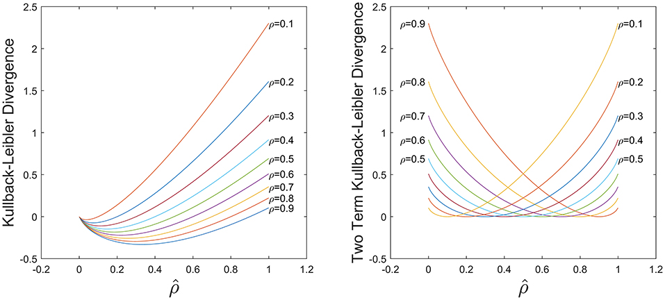
Figure 2. Comparison of KL divergence in Equation (5) using only the first term (Left) and the both terms (Right). With both terms the KL divergence is non-negative and symmetric for $\widehat{\rho }=0.5$.

Combining Equations (1), (3), (4), and (5) we obtain a total cost function used to train the deep sparse autoencoder defined as.

$\begin{array}{ll}E=ϵ+\lambda {\Omega }_w+\beta {\Omega }_s.& (6)\end{array}$

2.4. Cluster Segmentation

Once we have obtained a low dimensional representation of the data we can identify any patterns of the encoded features in the CMR data and determine the attributes that are driving the formation of any sub-groups. In selecting a deep autoencoder with a dimensionality of three in the encoded space with the lowest number of dimensions, we can visualize this representation of the data as a scatter plot. This is common in high dimensional visualization, classification, or deep learning tasks as it can reveal patterns in the data such as separation of groups into clusters, or location on a manifold. The low dimensional representation of the data exhibits clustering of CMR data (Figure 3), indicating that points within each cluster share commonalities in their features. Typically, analysis of these data representations are qualitative comparisons of different embedding methods [24, 32], or they provide the basis for training classification algorithms [17, 18] when the class labels are available. In our case we do not have labeled data and hence we can not use the labels of data points as an indicator of the network's performance. However, we can compare the data points within each cluster to identify what features are driving their formation in the low dimensional space. To isolate points within each cluster we segment the RGB space using a mesh to divide the co-ordinate space into regions of fixed size boxes, and discard regions with no data points. This isolates the vast majority of the clusters as illustrated in Figure 3B). Resulting clusters are manually inspected and corrected for instances of cluster splitting or merging. Thresholding for clusters with more than 5 data points yields 27 unique clusters of CMR data points in the RGB space. We note it is possible to perform clustering on the low dimensional data; however, we found that even with a variety of distance metrics, k-means over or under segmented the clusters in the data. The exploration of automated clustering methods is an obvious extension though is not the focus of this current study.

FIGURE 3

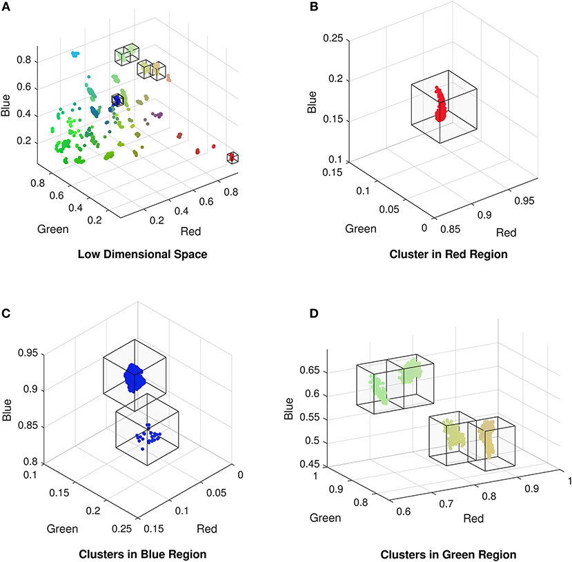
Figure 3. (A) Low dimensional representation of the CMR data following reduction with the autoencoder exhibiting the formation of clusters of CMR data. Isolated clusters in the (B) red, (C) blue, and (D) green regions of the low dimensional (RGB) space (omitting empty regions for clarity).

2.5. Analysis Using Shannon Entropy

Although segmenting the clustered data allows us to identify the attributes driving these clusters, and therefore patterns in the data, this does not explicitly provide a rationale for variations in cluster sizes, density or proximity to neighbors. One can make quality assessments of a larger cluster size indicating more variable or heterogeneous data, though this can be inappropriate if the low dimensional coordinate space contains nonlinearities, non-constant intervals or dimensions, or is poorly understood [33]. Moreover, the mixed data types can compound the problem of determining data variance or heterogeneity if using different measures for each data type. However, by interpreting the clusters as probability distributions we can make use of Shannon Entropy [34], H, defined as

$\begin{array}{ll}H(X)=𝔼\left[-log(P(X))\right]=-{\displaystyle \sum _i^n}P(x_i){log}_{b}P(x_i),& (7)\end{array}$

where P(x_i) is the probability of x_i and b=2. This enables the calculation of H(X) when X is numerical, categorical, date, or text data by computing the number of possible outcomes, and their frequencies, within cluster X. Using the groups in the data identified by the DAE in Figure 3, we can select the subset of the original CMR data and compute H(X) for each attribute within this subset. A low entropy (H(X) → 0) occurs when the majority of members in the subset have the same value, i.e., there is a narrow distribution of values, and H(X) = 0 when all data points have the same value for a given attribute. In contrast, a high entropy (H(X) → ∞) indicates a lack of commonality between members and the subset has a wide distribution of values for a given attribute in the CMR data. Comparing the entropy values for all CMR subsets identified in Figure 3, we can identify the attributes that are driving the formation of the clusters by comparing those that have low entropy values for cluster members but differ between clusters. Moreover, we can calculate H(X) for the clusters in the low dimensional space obtained from the deep autoencoder by interpreting the position of the points as a probability distribution. For very dense clusters, H(X) → 0, all cluster members occupy the same space, hence the autoencoder has identified a pattern of attributes that well characterize this sub-group in the dataset. Conversely, diffuse clusters, H(X) → ∞, are less ordered (more variable) and patterns identified by the network are less precise. This permits the comparison of different clusters within the data, and for each attribute, in order to identify the main drivers for the clusters. That is, in the case of CMR, we compute the entropy for the low dimensional clusters, and the individual attributes in the original high dimensional data (e.g., Gender, Age, etc.) to identify how the attributes are contributing to the entropy in the low dimensional space.

We implement our algorithms and all subsequent analysis in MATLAB (MathWorks, 2016a) using the deep learning toolbox and custom codes.

3. Results

We find that $\widehat{\rho }$=0.5 yields the best performance for CMR data as a balance between specialization and generalization in the hidden layers, leading to the formation of well defined clusters. A network with too few layers may not be able to capture complex patterns in the data, however, beyond the four layers in Figure 3 additional layers do not noticeably improve the low dimensional representation and increased computational cost for training. When training the network, we find that a ReLU activation function is unable to train a network that can learn an interesting representation of the data in the low dimensional space under any combination of hyper-parameters. This activation function learns a low dimensional representation of the data that embeds all the data points into the same space, i.e., all 11,000 CMR are indistinguishable. It is unclear if this is a result of the pre-processing of the CMR data required to enable training a DAE for these data, or whether optimization of structure and hyper-parameters using meta-heuristic algorithms are needed in this case. In contrast we find that a Sigmoid activation function captures interesting patterns in the data that are unobtainable with a ReLU activation function (see Figure 4).

FIGURE 4

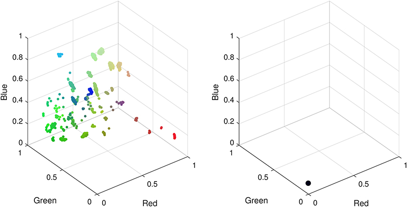
Figure 4. Low dimensional representations of CMR data with a deep autoencoder using sigmoid (Left) and ReLU (Right) activation functions. Using a sigmoid activation function patterns identified by the network manifest as clusters in the low dimensional space. When using a ReLU function all data points are confined to the same low dimensional space hence there are no observable patterns to differentiate the CMR data.

Training the network to encode these data had a computational runtime of (69.67 ± 2.42) seconds where the uncertainty is the standard error in the mean over 10 independent training cycles using the same network configuration and parameters. This does not include optimization of hyper-parameters. Once trained, the network provides a deterministic method to encode and decode the input data, or unseen data, that will ensure results are reproducible and directly comparable. This provides a very efficient means to analyse CMR as the encoding and decoding times are (0.157 ± 0.002) and (0.193 ± 0.009) seconds, respectively, for 11,000 CMR. Using pre-trained networks could serve as a practical tool for medical practitioners and clinicians to use for real time analysis of CMR data based on cluster membership in the low dimensional representation. Moreover, the training time is approximately 70 s when trained on a CPU, hence there is opportunity to utilize GPUs and further optimizations to enable dataset specific training for CMR data in reasonable time frames to be practical in healthcare settings.

The reduction to three dimensions permits visualization of the CMR data as a 3D scatter plot where the (x, y, z) coordinates can be interpreted as red-blue-green (RGB) as exhibited in Figure 3 where the clusters vary in size and dispersion. We segment the low dimensional space to isolate the clusters using a fixed size mesh yielding 27 individual sub-groups, with the data using a minimum cluster size of five points (0.05% of the dataset, summarized in Table 1). The clustered data represent 97.84% of the CMR data.

TABLE 1

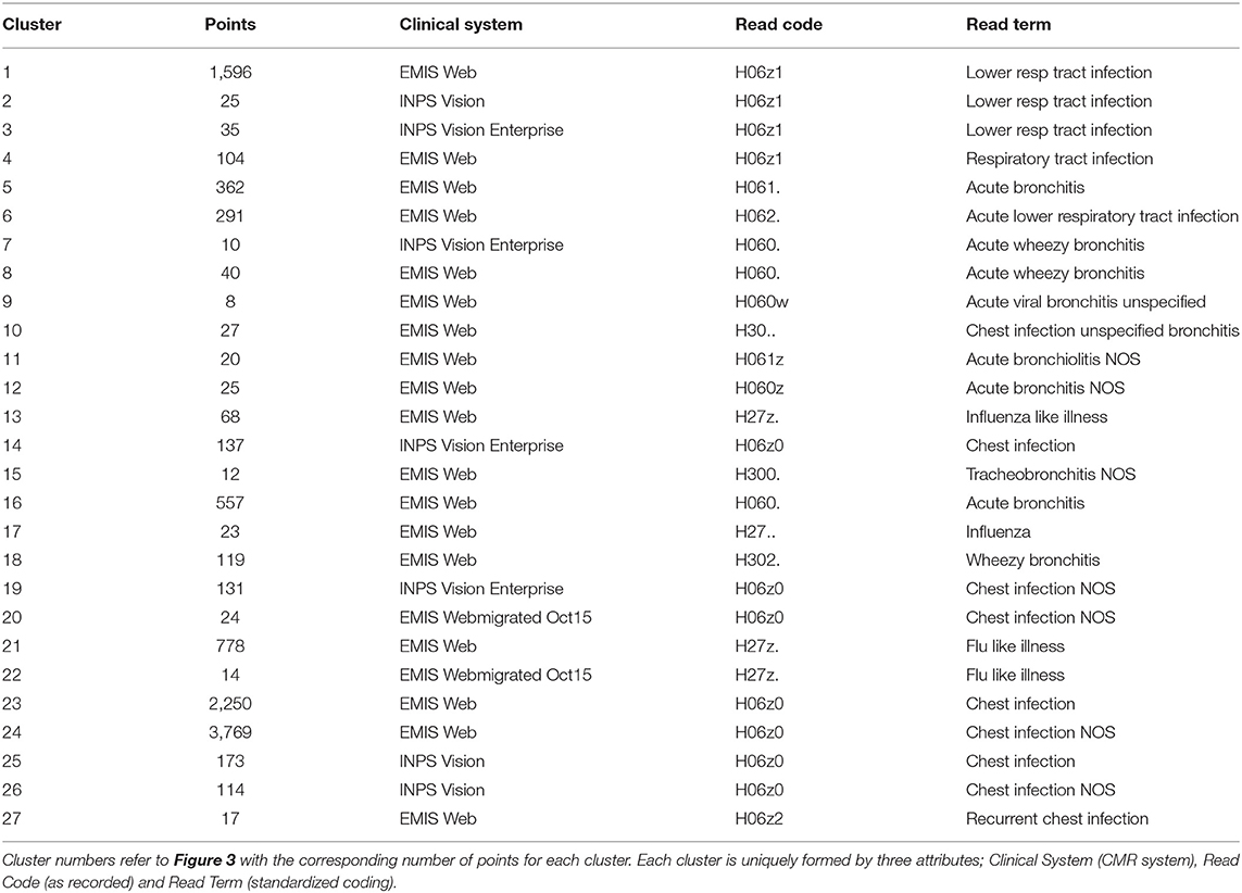
Table 1. Key attributes in driving formation of clusters covering 97.84% of the data.

We can compute the entropy of each cluster in the low dimensional space based on the RGB values of each data point (defined by the x, y, z co-ordinates) they contain. Using the cluster labels identified using the DAE and the segmentation method, we can extend the entropy analysis to the original CMR data attributes collectively and individually. Computing the entropy for each attribute for the members within the clusters can identify greatest contribution to cluster dispersion in the low dimensional representation. Entropy is a measure of a disordered system; in this context disorder can be interpreted as variability in the data. A high entropy occurs when there is a broad distribution of values within a set of data points; i.e., when points in a cluster do not share a common attribute. A low entropy on the other hand is indicative of a well ordered cluster where the majority of points have a common attributes. In the case where entropy equals zero, all points in a cluster have the same value. This is useful in identifying the features in the CMR data that are driving the patterns in the low dimensional data, resulting in the formation of clusters as those with zero entropy contain specific attribute values in the cluster. Analysing each cluster reveals that all of them can be uniquely identified through a combination of only three of the attributes, namely, Clinical System, Read Code and Read Term, each of which has zero entropy for each cluster (see Table 1). Interestingly, of all the values available for each of the three main attributes driving the formation of clusters, only a few are required to uniquely identify 98% of the data. All the remaining data are disparate points or form clusters with fewer than five data points. In addition, identifying the attributes with the highest entropy provides insight into the features that have little or no influence in forming these low dimensional patterns. The least ordered attributes are typically Practice ID, Event Date and Age indicating that these are the attributes with the highest variability. The implication of this is that these features do not influence cluster membership, but they are however the largest contributors to the cluster dispersion in Figure 3.

The entropy of a specific attribute provides useful information about how that feature is contributing to the variability in the low dimensional space, but we can also sum the entropy for each feature to indicate the variability of a sub-group of CMR data. Taking each cluster as a sub-group and summing the entropy for each of the attributes within each cluster provides an indication of the variability of the original high dimensional input data. Interestingly, this summed entropy correlates strongly with the entropy of the low dimensional RGB points with a Pearson's Correlation of 0.99 and an R² of 0.98 as shown in Figure 5. The low dimensional representation of the CMR data learned by the DAE has not only identified structure in the data, but also maintains the properties of the original high dimensional data. This indicates that the DAE can produce visualizations that accurately reflect the input data that can be further analyzed as outlined here.

FIGURE 5

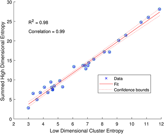
Figure 5. Relationship between the entropy of low dimensional clusters in Figure 3A and the entropies of the high dimensional CMR data (summed over all attributes). The data (blue crossed circles) have a high Pearson's correlation of 0.99 and follow a linear fit (solid red line) with an R² of 0.98 and a narrow 95% confidence bound (dashed red line) as indicated.

4. Discussion and Conclusions

The analysis of the CMR data with a deep autoencoder was able to isolate sub-groups within the dataset that can be uniquely identified by three of the attributes. The other six attributes were found to not affect the formation of clusters, only their diffuseness. The lack of influence of Practice ID, Event Date, Age and Gender in grouping the data indicate the absence of a systematic bias in the data recording. That is, clusters forming based on these variables would indicate these as major discriminating features. As neither Practice ID nor Event Date discriminate the data in any observable way we can be confident that the data are well standardized and that practices and personnel recording the data are not an influence in any observable patterns.

The ratio of genders in each cluster varies between 1:1 and 3:1 but also does not significantly segment the data in an observable way. 14 of the clusters contain ≥ 60% females, 10 of the clusters are 50:50 males to females, and the remaining 3 clusters ≥ 60% males. This does not take in to account the difference in cluster population size, or instance of multiple CMRs from the same patient, though this type of further analysis is possible. For other datasets, gender may be an important factor, such as in certain types of disease, however it is not found to be influential in grouping patients with respiratory conditions as we would expect. The Coding System has the same values for all but one instance in the datasets thus has no influence on the results and is omitted from our analysis and summaries. Looking at the distribution of Episode type for each of the clusters we can identify some archetypal patterns in the data. Of all 27 clusters in the data we observe 5 general trends in the data summarized in Figure 6; (a) one with ≈ 50% new (N) and first (F), (b) seven clusters with >70% missing (M), (c) 13 clusters with >59 % F, (d) five clusters with ≈ 50% F, and ≈ 20% O, and (e) one cluster with ≈ 50% ongoing (O). A typical distribution of Episode type with these patterns is illustrated in Figure 6 for a few of the clusters. These distributions are useful in assessing the subsets of data with missing entries or the ratio of first and new to ongoing Episodes. We can further analyse the cluster with the highest proportion of missing Episode type in order to identify trends in the data such as the sources of these CMRs. The largest proportion of data with missing Episode type are from the INPS Vision and INPS Vision Enterprise Clinical Systems (Table 2). Data from the EMIS systems contain much fewer missing data providing better quality input for the Weekly Returns Service and any data for predictive models. We note that the TTP systmOne constitute only 38 out of 11,000 records and did not form clusters larger than 5 data points and so does not appear in our analysis. This analysis is useful in identifying common features in CMRs and data sources, and provide potential early warning signs as larger proportions of incident (first and new) Episodes can be used to detect potential disease outbreaks to prevent epidemics. Implementation of this system could enable targeted analysis of the data focusing on specific ages or regions through Practice ID, or a front end for data correction methods [20] for improved reporting and forecasting.

FIGURE 6

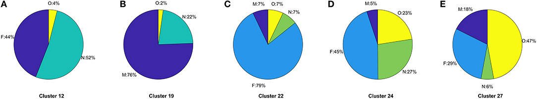
Figure 6. (A–E) Typical distributions of Episode for the five archetype clusters in CMR data identified in Figure 3 listing the specific cluster the distribution arises from. Pie charts illustrate the frequency of Episode type and the proportion of missing (M), first (F), new (N), or ongoing (O) occurrence of respiratory infection listed in the CMR data.

TABLE 2

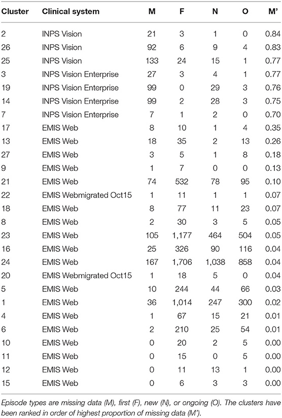
Table 2. Rank clusters by highest proportion of missing Episode type.

We note that the identification of three main drivers is not dependent on the number of dimensions in our DAE as these attributes vary in dimensionality. The input data consists of a concatenated vector of the attributes in the CMR converted, described in section 2.2, with a total dimensionality of 93, where the three attributes driving the clusters (Read Term, Clinical System and Read Code) contributing 58%, 24% and 5%, respectively, to the dimensionality of the input. Once the attributes are combined there is no distinction between elements in the input vector. Moreover, the contribution of each element is restricted by using a sparse DAE as outlined in section 2.3, which limits the dominance of any particular entry in the input vector.

In this work we have presented a methodology for processing heterogeneous CMR data and performed unsupervised nonlinear dimensionality reduction using a deep autoencoder. Analysing the data in this way enables the visualization and segmentation of the high dimensional multi-type CMR data in order to identify patterns and trends in the data. From these, we can carry out cluster specific analysis. This efficient methodology can perform reduction of the data at a practical time scale to be a useful tool for healthcare practitioners. Furthermore, we introduce the use of Shannon Entropy as a means to analyse the variability of heterogeneous CMR data. Furthermore, we show a strong correlation between the Shannon Entropy in both the original CMR and DAE reduced data, demonstrating that the low dimensional clusters are representative of the original data. Maintaining properties of the CMR data in the low dimensional representation enables confidence in further analysis such as interpretation of visualizations and variability, that is not possible in other nonlinear reduction techniques [33].

These methods can be combined with methods for data correction. This is a vital benefit, as 15–20 practices (50,000–150,000 patients) are excluded from the RCGP Weekly Returns Service due to being poor quality data [20]. The Weekly Returns Service monitors the number of patients with incident Episodes of illness in England and is the key primary care element of the national disease monitoring systems run by Public Health England [20]. The analysis of this data are also critical for assessing flu vaccine effectiveness [4], hence the omission of such a large amount of data each week is significant, and methods for data correction are of high importance.

The data used here are examples of data selected over a 6 week period from 230 practices, however the methodology can be extended to large subsets of the database to identify further patterns in the data. An investigation over a longer time frame may identify any slow dynamic trends such as periodic changes in data quality. The results presented here have shown the benefit of this type of analysis for CMR data and its use for near real time data analysis. This methodology has the potential to be used by medical practitioners to aid data analysis and decision making such as treatment course or diagnosis, though more work is needed in understanding and optimizing the algorithm. The use of regularization plays a vital role in the training process and the embedded results, though it is unclear how to select an appropriate regularization strategy or their coefficients in the cost function. A comparison between other regularization methods, such as L1-norm, would be particularly useful due to its promotion of sparsity [35]. Comparison of our sparse deep autoencoder to other sparse methods such as compressed sensing would also be of interest for these data.

Ethics Statement

This study has been approved by the Royal College of General Practitioners research and surveillance centre. Specific ethics committee approval is not required as there will be no direct patient contact in this study, and the data will not be patient identifiable.

Author Contributions

RW, IY, and SdL collected and provided the data. ST, NS, VL, and SdL defined the experimentation. ST carried out the method development and data analysis. All authors contributed to the interpretation of results and preparing the manuscript, and completed appropriate information governance training. All data used in this work was fully anonymised and complies with the RCGP protocols and ethics.

Funding

This work was funded by the department of Business, Engineering and Industrial Strategy through the cross-theme national measurement strategy (Digital Health, 121572).

Conflict of Interest Statement

The authors declare that the research was conducted in the absence of any commercial or financial relationships that could be construed as a potential conflict of interest.

Acknowledgments

Patients and practices of RCGP RSC who consent to share data. Apollo medical systems and CMR suppliers – EMIS, TPP, In Practice Systems. The authors would like to thank Louise Wright and Jennifer Livings for valuable feedback on the manuscript.

Abbreviations

CMR, Computerized medical records; DAE, deep autoencoder; RCGP, Royal College of General Practitioners; RSC, Research and Surveillance Centre.

References

1. Thomas SA, Jin Y. Reconstructing biological gene regulatory networks: where optimization meets big data. Evol Intell. (2014) 7:29–47. doi: 10.1007/s12065-013-0098-7

CrossRef Full Text | Google Scholar

2. Fleming DM, Schellevis FG, Paget WJ. Health monitoring in sentinel practice networks: the contribution of primary care. Eur J Public Health. (2003) 13:84. doi: 10.1093/eurpub/13.suppl_3.80

PubMed Abstract | CrossRef Full Text | Google Scholar

3. Souty C, Turbelin C, Blanchon T, Hanslik T, Le Strat Y, Boëlle PY. Improving disease incidence estimates in primary care surveillance systems. Populat Health Metrics. (2014) 12:19. doi: 10.1186/s12963-014-0019-8

PubMed Abstract | CrossRef Full Text | Google Scholar

4. Correa A, Hinton W, McGovern A, van Vlymen J, Yonova I, Jones S, et al. Royal college of general practitioners research and surveillance centre (RCGP RSC) sentinel network: a cohort profile. BMJ Open. (2016) 6. doi: 10.1136/bmjopen-2016-011092

PubMed Abstract | CrossRef Full Text | Google Scholar

5. de Lusignan S, Correa A, Smith GE, Yonova I, Pebody R, Ferreira F, et al. RCGP research and surveillance centre: 50 years' surveillance of influenza, infections, and respiratory conditions. Brit J Gen Pract. (2017) 67:440–1. doi: 10.3399/bjgp17X692645

PubMed Abstract | CrossRef Full Text | Google Scholar

6. Fleming DM, Elliot AJ. Lessons from 40 years' surveillance of influenza in England and Wales. Epidemiol Infect. (2007) 136:866–75. doi: 10.1017/S0950268807009910

PubMed Abstract | CrossRef Full Text | Google Scholar

7. Fleming DM, Durnall H. Ten lessons for the next influenza pandemic—an English perspective. Hum Vaccines Immunotherapeut. (2012) 8:138–45. doi: 10.4161/hv.8.1.18808

PubMed Abstract | CrossRef Full Text | Google Scholar

8. de Lusignan S, van Weel C. The use of routinely collected computer data for research in primary care: opportunities and challenges. Fam Pract. (2006) 23:253–63. doi: 10.1093/fampra/cmi106

PubMed Abstract | CrossRef Full Text | Google Scholar

9. Gordon D, Bone A, Pebody R, de Lusignan S. The GP's role in promoting winter wellness. Br J Gen Pract. (2017) 67:52–3. doi: 10.3399/bjgp17X688909

PubMed Abstract | CrossRef Full Text | Google Scholar

10. Pebody RG, Green HK, Warburton F, Sinnathamby M, Ellis J, MÃlbak K, et al. Significant spike in excess mortality in England in winter 2014/15 – influenza the likely culprit. Epidemiol Infect. (2018) 146:1106–13. doi: 10.1017/S0950268818001152

PubMed Abstract | CrossRef Full Text | Google Scholar

11. Ulloa A, Basile A, Wehner GJ, Jing L, Ritchie MD, Beaulieu-Jones B, et al. An unsupervised homogenization pipeline for clustering similar patients using electronic health record data. ArXiv e-prints (2018).

Google Scholar

12. Thomas SA, Lloyd DJB, Skeldon AC. Equation-free analysis of agent-based models and systematic parameter determination. Physica A. (2016) 464:27–53. doi: 10.1016/j.physa.2016.07.043

CrossRef Full Text | Google Scholar

13. Martin R, Thomas SA. Analyzing regime shifts in agent-based models with equation-free analysis. In: International Congress on Environmental Modelling and Software. Toulouse (2016). p. 494–502. Available online at: https://scholarsarchive.byu.edu/iemssconference/2016/Stream-B/54

Google Scholar

14. Kevrekidis IG, Samaey G. Equation-free multiscale computation: algorithms and applications. Annu Rev Phys Chem. (2009) 60:321–44. doi: 10.1146/annurev.physchem.59.032607.093610

PubMed Abstract | CrossRef Full Text | Google Scholar

15. Guan WJ, Jiang M, Gao YH, Li HM, Xu G, Zheng JP, et al. Unsupervised learning technique identifies bronchiectasis phenotypes with distinct clinical characteristics. Int J Tubercul Lung Dis. (2016) 20:402–10. doi: 10.5588/ijtld.15.0500

PubMed Abstract | CrossRef Full Text | Google Scholar

16. LeCun Y, Bengio Y, Hinton G. Deep learning. Nature. (2015) 521:436–44. doi: 10.1038/nature14539

PubMed Abstract | CrossRef Full Text | Google Scholar

17. Hinton GE, Salakhutdinov RR. Reducing the dimensionality of data with neural networks. Science. (2006) 313:504–7. doi: 10.1126/science.1127647

PubMed Abstract | CrossRef Full Text | Google Scholar

18. Thomas SA, Jin Y, Bunch J, Gilmore IS. Enhancing classification of mass spectrometry imaging data with deep neural networks. In: 2017 IEEE Symposium Series on Computational Intelligence (SSCI). Athens (2017). p. 1–8.

Google Scholar

19. Avati A, Jung K, Harman S, Downing L, Ng A, Shah NH. Improving palliative care with deep learning. ArXiv e-prints (2017). doi: 10.1109/BIBM.2017.8217669

PubMed Abstract | CrossRef Full Text | Google Scholar

20. Smith N, Livina V, Byford R, Ferreira F, Yonova I, de Lusignan S. Automated differentiation of incident and prevalent cases in primary care computerised medical records (CMR). Stud Health Technol Informat. (2018) 247:151–5. doi: 10.3233/978-1-61499-852-5-151

PubMed Abstract | CrossRef Full Text | Google Scholar

21. Møller MF. A scaled conjugate gradient algorithm for fast supervised learning. Neural Netw. (1993) 6:525–33. doi: 10.1016/S0893-6080(05)80056-5

CrossRef Full Text | Google Scholar

22. Thomas SA, Race AM, Steven RT, Gilmore IS, Bunch J. Dimensionality reduction of mass spectrometry imaging data using autoencoders. In: 2016 IEEE Symposium Series on Computational Intelligence (SSCI). Honolulu, HI (2016). p. 1–7.

Google Scholar

23. van der Maaten L. Learning a parametric embedding by preserving local structure. In: van Dyk D, Welling M, editors. Proceedings of the Twelth International Conference on Artificial Intelligence and Statistics. vol. 5 of Proceedings of Machine Learning Research (PMLR). Clearwater, FL (2009). p. 384–91.

Google Scholar

24. van der Maaten L, Hinton G. Visualizing data using t-SNE. J Mach Learn Res. (2008) 9:2579–605. Available online at: http://www.jmlr.org/papers/volume9/vandermaaten08a/vandermaaten08a.pdf

Google Scholar

25. Fonville JM, Carter CL, Pizarro L, Steven RT, Palmer AD, Griffiths RL, et al. Hyperspectral visualization of mass spectrometry imaging data. Anal Chem. (2013) 85:1415–23. doi: 10.1021/ac302330a

PubMed Abstract | CrossRef Full Text | Google Scholar

26. Shared and distinct transcriptomic cell types across neocortical areas. Nature. (2018) 563:72–8. doi: 10.1038/s41586-018-0654-5

CrossRef Full Text

27. Mahfouz A, van de Giessen M, van der Maaten L, Huisman S, Reinders M, Hawrylycz MJ, et al. Visualizing the spatial gene expression organization in the brain through non-linear similarity embeddings. Methods. (2015) 73:79–89. doi: 10.1016/j.ymeth.2014.10.004

PubMed Abstract | CrossRef Full Text | Google Scholar

28. Highly parallel genome-wide expression profiling of individual cells using nanoliter droplets. Cell. (2015) 161:1202–14. doi: 10.1016/j.cell.2015.05.002

CrossRef Full Text

29. Krogh A, Hertz JA. A simple weight decay can improve generalization. In: Advances in Neural Information Processing Systems 4. Colorado: Morgan Kaufmann (1992). p. 950–7.

Google Scholar

30. Hassoun M. Fundamentals of Artificial Neural Networks. Cambridge, MA: MIT Press (1995).

Google Scholar

31. Loone SM, Irwin G. Improving neural network training solutions using regularisation. Neurocomputing. (2001) 37:71–90. doi: 10.1016/S0925-2312(00)00314-3

CrossRef Full Text | Google Scholar

32. van der Maaten L. Barnes-Hut-SNE. CoRR. (2013) abs/1301.3342. Available online at: http://arxiv.org/abs/1301.3342

33. Wattenberg M, Viégas F, Johnson I. How to use t-SNE effectively. Distill. (2016). Available online at: http://distill.pub/2016/misread-tsne

Google Scholar

34. Shannon CE. A mathematical theory of communication. Bell Syst Tech J. (1948) 27:379–423. doi: 10.1002/j.1538-7305.1948.tb01338.x

CrossRef Full Text | Google Scholar

35. Ng AY. Feature selection, L1 vs. L2 regularization, and rotational invariance. In: Proceedings of the Twenty-first International Conference on Machine Learning. ICML '04. New York, NY: ACM (2004). p. 78–86.