A General Model for Both Shape Control and Locomotion Control of Tensegrity Systems

Introduction

Tensegrity systems are a class of special prestressed pin-jointed bar assembly, composed of compression elements and tension elements. A distinguishing feature of tensegrity structures is that their shape and mechanical properties can be actively controlled by prestressing their structural elements, making them good candidates for structural systems requiring controllable shapes and mechanical properties, such as smart structures (Shea et al., 2002; Fest et al., 2003; Motro, 2003; Al Sabouni-Zawadzka, 2014), deployable structures (Fazli and Abedian, 2011; Veuve et al., 2015; Kan et al., 2018; Oh et al., 2018), tunable metamaterials (Fraternali et al., 2014; Amendola et al., 2018; Liu et al., 2019), and robots (Paul et al., 2006; Mirletz et al., 2015; Kim et al., 2017; Cera and Agogino, 2018; Park et al., 2019; Wang et al., 2019). The actuators of a controllable tensegrity structure can usually be idealized as active members with variable rest lengths. The main problem to be solved in the control of a tensegrity system given an actuation configuration is determining the actuations (i.e., rest length changes of the active members) required to drive the structural system from its initial state to the target state.

If the actuations are imposed on the structural system very slowly and the structural system remains in static equilibrium throughout the control process, it is deemed a quasi-static system and the control problem can be interpreted as that of finding a static equilibrated path to connect the initial and target states. Most recent studies on shape control of tensegrity structures have treated it as a quasi-static process (Shea et al., 2002; Sultan et al., 2002; Xu et al., 2014). In particular, the prestressable equilibrium manifold of symmetrical prism tensegrity structures can be identified analytically, and then feasible control paths can be determined based on the equilibrium manifold using a search strategy (Sultan et al., 2002; Sultan and Skelton, 2003). For general cases in which the equilibrium manifold cannot easily be determined, an algorithm based on rapidly-exploring random trees has been proposed to find feasible actuation sets for the shape control of tensegrity systems (Xu et al., 2014). Form-finding methods, such as dynamic relaxation method (Fest et al., 2003) and non-linear force method (Xu and Luo, 2009) have been used to track the quasi-static motion of shape controlled tensegrities. Meanwhile, the dynamic effect have to be considered in the studies of locomotive tensegrity systems, due to the stronger actuations and environmental interactions involved in such systems. The potential for using tensegrity structures as locomotive systems has recently attracted considerable attention. A tensegrity swimmer was developed to achieve propulsive performance with closed-loop control (Bliss et al., 2013). Omer et al. (2011) proposed a 2D tensegrity robot to mimic caterpillar locomotion. Böhm and Zimmermann (2013) proposed a vibration-driven mobile tensegrity robot. The DuCTT (Duct Climbing Tetrahedral Tensegrity) with the ability to traverse complex duct systems was presented and demonstrated (Friesen et al., 2014, 2016). Spherical tensegrity robots with potential application in planetary explorers (SunSpiral et al., 2013; Sabelhaus et al., 2015) have been most intensively studied (Khazanov et al., 2013; Kim, 2016; Luo and Liu, 2017; Lu et al., 2019). To track the dynamic motion of locomotive tensegrities, Runge-Kutta method (Rovira and Tur, 2009), multi-body kinematic and dynamic simulation (Lin et al., 2016), and commercial physical engine (Zhao et al., 2017) have been used. Different descriptions and formulations are usually used for the shape control and the locomotion control problems of tensegrity systems, due to the difference in their application scenarios and the difference in the academic background of the researchers. In this paper, both the shape controlled tensegrity systems and the locomotive tensegrity systems will be modeled by the same mathematical formulations and a DRM-based motion tracking algorithm applicable for both quasi-static and dynamic motions will be adopted.

This paper is laid out as follows: section Model for Controllable Tensegrity Systems presents the general mathematical model for controllable tensegrity systems. In section Control Optimization Method, a method incorporating a GA-based optimization scheme with a DRM-based motion tracking algorithm is developed to solve the model. The proposed model and method are implemented in a tensegrity system shape control application in section Shape Control. Section Locomotion Control presents the application of the proposed model and method to locomotive control in tensegrity systems. Finally, section Discussion concludes the study.

Model for Controllable Tensegrity Systems

For a tensegrity system composed of n nodes and n_c elements, an element's type is given by the element type vector D = [D₁, D₂, …, D_nc] where D_i is defined as:

$\begin{array}{ll}{D}_i=\{\begin{array}{c}1,forcompressionelement\\ 0,fortensionelement\end{array}& (1)\end{array}$

For a controllable tensegrity system with n_a (n_a ≤ n_c) active elements, the locations of the active elements are described by an active element location vector D_A = [D_A1, D_A2, …, D_{A nc}], where

$\begin{array}{ll}{D}_{Ai}=\{\begin{array}{c}1,foractiveelement\\ 0,forpassiveelement\end{array}& (2)\end{array}$

in which “active element” means the element whose length can be actively changed by actuators, and “passive element” means the element whose length cannot be actively changed. The active element location vector satisfies that sum (D_A) = n_a.

The control strategy of a controllable tensegrity system can be described by an actuating function Δ. During a given time period [t_s, t_f], the actuating function of the i^th member is defined as e_i = f_i(t), where f_i is a continuous function of time t. Then, the actuating function Δ is written as

$\begin{array}{ll}\Delta =\left\{e_1,e_2,\dots ,e_{n_c}\right\}& (3)\end{array}$

where $e_i\in \left[-e_i^s,e_i^l\right]$, in which $e_i^s$ and $e_i^l$ are the allowable shortening and elongation for the i^th member, respectively. Note that $e_i^s=$ $e_i^l=$ 0 for passive members (D_Ai = 0). The rest length change ranges of the elements can be expressed as $\text{E}=\left\{\left[-e_1^s,e_1^l\right],\left[-e_2^s,e_2^l\right],\dots ,\left[-e_{n_c}^s,e_{n_c}^l\right]\right\}$. Hence, at any time, the rest length change function of the controllable tensegrity system is required to satisfy the condition that Δ ∈ E.

The rest length of members ${\text{L}}_R^t$ at time t satisfies

$\begin{array}{ll}{\text{L}}_R^t={\text{L}}_R^{t_s}+{\Delta }^t& (4)\end{array}$

The internal force $F_i^t$ of the i^th member is determined by

$\begin{array}{ll}{F}_i^t=\frac{E_i{A}_i\left(L_{Gi}^t-L_{Ri}^t\right)}{L_{Ri}^t}& (5)\end{array}$

where E_i, A_i, $L_{Gi}^t$, and $L_{Ri}^t$ are the elasticity modulus, cross-sectional area, deformed length, and rest length of the i^th member, respectively. Meanwhile, the internal force $F_i^t$ of the i^th member is required to be within the strength limitations, i.e.,

$\begin{array}{ll}{F}_i^l\le F_i^t\le F_i^u& (6)\end{array}$

where $F_i^l$ and $F_i^u$ are the lower bound and upper bound of the strength of the i^th member, respectively. Specifically, $F_i^l$ and $F_i^u$ are given by

$\begin{array}{l}{F}_i^l=–\text{min}(F_{ci},F_{bi})and{F}_i^u=0,for{D}_i=1\\ F_i^l=0and{F}_i^u=F_{ti},for{D}_i=0& (7)\end{array}$

where F_ci, F_bi, and F_ti are the compression strength, buckling strength, and tension strength of the i^th member, respectively. Having defined ${\Omega }_{\text{f}}=\left\{\left[F_1^l,F_1^u\right],\left[F_2^l,F_2^u\right],\dots ,\left[F_{n_c}^l,F_{n_c}^u\right]\right\}$, the strength constraint on the members of the controllable tensegrity system can be written as ${\text{F}}^t\in {\Omega }_{\text{f}}$.

The equilibrium equation of the tensegrity system at time t is written as

$\begin{array}{ll}{\text{A}}^t{\text{F}}^t={\text{F}}_e^t& (8)\end{array}$

where A^t (n_r × n_c) is the equilibrium matrix, F^t_e (n_r × 1) is the external nodal load vector, and n_r is the number of degrees of freedom. Hence, the unbalanced nodal force R^t of the system at time t can be expressed as

$\begin{array}{ll}{\text{R}}^t={\text{F}}_e^t-{\text{A}}^t{\text{F}}^t& (9)\end{array}$

Then, according to Newton's second law:

$\begin{array}{ll}{\text{R}}^t=\text{M}{\ddot{\text{U}}}^t+\text{C}{\dot{\text{U}}}^t& (10)\end{array}$

where M is the nodal mass matrix of the system, C is the viscous damping of the system, and U is the matrix of nodal coordinates of the system.

Substituting Equation (9) into Equation (10) yields

$\begin{array}{ll}{\text{F}}_e^t-{\text{A}}^t{\text{F}}^t=\text{M}{\ddot{\text{U}}}^t+\text{C}{\dot{\text{U}}}^t& (11)\end{array}$

The control objective of the system is case-dependent. It could be a special requirement of the nodal displacement, locomotion distance, or the energy cost to generate the required shape adjustment or motion. Since it is usually a function of the control strategy, it can be conceptually represented as G(Δ).

Based on the above definitions of the control strategy, constraints, and control objective, a general model for the controllable tensegrity system can be written as

$\begin{array}{ll}\{\begin{array}{l}find\Delta \\ minG(\Delta )\\ s.t.\\ {\text{F}}_e^t-{\text{A}}^t{\text{F}}^t=\text{M}{\ddot{\text{U}}}^t+\text{C}{\dot{\text{U}}}^t\\ \Delta \in \text{E}\\ \text{U}\in {\Omega }_{\text{s}}\\ {\text{F}}^t\in {\Omega }_{\text{f}}\\ C(\Delta )\end{array}& (12)\end{array}$

where Ω_s represents free space in an environment where the controllable system does not interfere with boundaries or obstacles, and C(Δ) represents the additional constraints on the system in specific situations.

Control Optimization Method

Motion Tracking

An incremental procedure based on the dynamic relaxation method (Xu and Luo, 2013) is adopted to simulate the motion of the controllable tensegrity system under a given actuation. The duration of the actuation is discretized by a given time increment of Δt. The state of the system is tracked by a DRM procedure that starts from a known state at time t and ends with a new state at time t + Δt after a time increment of Δt. Step by step, the motion of the system under the given actuation is discretely depicted. Details of the DRM-based motion tracking procedure are given in the following paragraph.

Under a given actuation Δ^t, the residual force R^t of the system is determined by Equation (9). According to Equation (10), for a node j in the direction x at time t, we have

$\begin{array}{ll}{R}_{jx}^t=M_j{\ddot{u}}_{jx}^t+C_{jx}{\dot{u}}_{jx}^t& (13)\end{array}$

where $R_{jx}^t$ represents the residual force of node j in the direction x, and is a component of R^t; M_j represents the equivalent nodal mass of node j; and C_jx represents the damping of node j in the direction x. The nodal acceleration can be approximated in centered finite difference form as

$\begin{array}{ll}{\ddot{u}}_{jx}^t=\frac{{\dot{u}}_{jx}^{t+\Delta t/2}-{\dot{u}}_{jx}^{t-\Delta t/2}}{\Delta t}& (14)\end{array}$

Substituting Equation (14) into Equation (13), the nodal velocity at t + Δt/2 can be expressed as

$\begin{array}{ll}{\dot{u}}_{jx}^{t+t/2}={\dot{u}}_{jx}^{t-\Delta t/2}+\frac{\Delta t}{M_j}(R_{jx}^t-C_{jx}{\dot{u}}_{jx}^t)& (15)\end{array}$

Then, the nodal coordinate at t + Δt can be expressed as

$\begin{array}{ll}{u}_{jx}^{t+\Delta t}=u_{jx}^{\Delta t}+{\dot{u}}_{jx}^{t+\Delta t/2}t& (16)\end{array}$

By setting t = t + Δt, the actuation Δ^t, equilibrium matrix A^t, internal force F^t, external force F^t_e, and residual force R^t can be updated accordingly. The above central difference process repeats until t = t_f. The numerical stability of this central difference process is guaranteed by using a time increment Δt no larger than $\sqrt{\frac{2M}{S}}$, where S is the highest direct stiffness of any node relative to adjacent nodes (Barnes, 1999). For quasi-static problems, the motion tracking can be interpreted as a series of form-finding processes (Xu and Luo, 2013). In each form-finding process, a sub-iteration scheme is implemented whereby each time step is iterated so that convergence is achieved for each time step (Senatore and Piker, 2015). Fictitious values for mass, stiffness, and damping are used to improve the performance of the algorithm for convergence to the static solution (Zhang et al., 2006). In particular, a technique called “kinetic damping” is usually adopted to expedite the convergence of algorithm (Barnes, 1999; Zhang et al., 2006). Note that the real value for stiffness should be substituted into the each form-found system to evaluate whether the stress and stability limits of the structural elements are met. For dynamic problems, real values for mass, stiffness, and damping are used by the algorithm. The effectiveness of it in dealing with dynamic problems has been demonstrated by a similar procedure called “finite particle method” (Yu and Luo, 2009; Yu et al., 2011). Note that a DRM-based scheme for both quasi-static analysis and dynamic analysis also has been proposed by Senatore and Piker (2015).

An internal collision-detecting strategy proposed in the literature (Xu et al., 2014) is used here to check whether there is internal collision between any pair of elements. This must be avoided, since any internal collision may cause the moving system to become stuck. As a result, the motion tracking algorithm stops if an internal collision is detected, and the path and corresponding actuation are deemed infeasible. On the other hand, collision between the structural system and its environment is allowed and must be accounted for. The penalty function method (Oden and Kikuchi, 1982; Papadopoulos and Taylor, 1992) is used to consider the interaction between the structural system and its environment. An obstacle in the environment is assumed to be a series of surfaces covered with springs, and the nodes of the tensegrity structure are allowed to penetrate the surface. The normal contact force F_n between the node and the surface is evaluated by

$\begin{array}{ll}{F}_n=k_n\delta & (17)\end{array}$

where δ is the penetration depth; and k_n is the virtual normal stiffness of the surface. The friction force F_f between the node and the surface is determined by

$\begin{array}{ll}{F}_f=\mu F_n& (18)\end{array}$

where μ is the friction coefficient.

Optimization Algorithm

To find a control strategy that minimizes the given objective, an optimization algorithm is required. The control problem modeled by Equation (12) is essentially a problem of combinatorial optimization, and the search domain is usually very large. Direct search algorithms such as evolutional algorithms, simulated annealing algorithms, and genetic algorithms are considered suitable for this problem. Without loss of generality, a genetic algorithm is adopted here.

Solution Flowchart

Combining the DRM-based motion tracking method and GA-based optimization algorithm, the flowchart of the algorithm is as shown in Figure 1. The main steps of the algorithm are as follows:

(1) Define the genetic representation and the fitness function; initialize a population.

(2) Decode the chromosomes.

(3) For each individual, build a numerical model of the corresponding tensegrity system for DRM; initialize the parameters of the numerical tensegrity model, and set t = t_s; perform Step (4) to Step (6).

(4) Apply a control strategy to the numerical tensegrity model through the actuating function Δ^t.

(5) Calculate the residual nodal force R^t; solve Equation (11) by the central difference method; update the nodal acceleration ${\ddot{\text{U}}}^t$, nodal velocity ${\dot{\text{U}}}^t$, and nodal coordinate U^t; apply constraints.

(6) If t = t_f, go to Step (7); otherwise, set t = t + Δt, and go to Step (4).

(7) Evaluate the fitness of the population. If the population satisfies the convergence condition or the number of generations reaches the maximum permissible, go to Step (9); otherwise, go to Step (8).

(8) Apply the selection, crossover, and mutation operators, and create a new generation. Then, go to Step (2).

(9) Output the solutions.

FIGURE 1

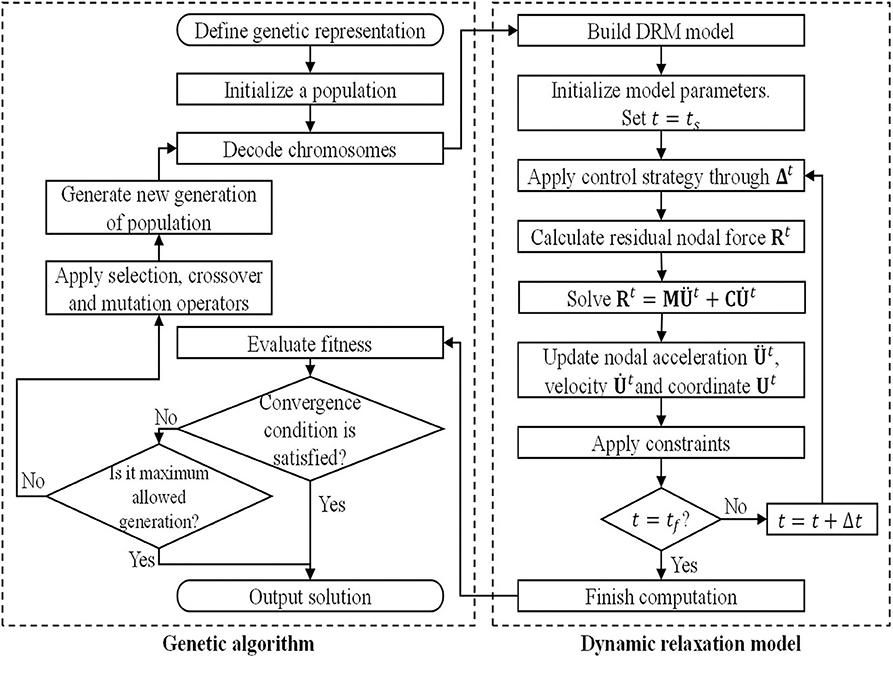
Figure 1. Flowchart of the solving method.

Shape Control

Shape-Controlled Tensegrity System

The feasibility of the proposed model and method in solving tensegrity system shape control problems is tested in a double-layered tri-prism tensegrity structure, which is used as a typical example of a shape-controlled tensegrity system in a previous study (Xu et al., 2014). As shown in Figure 2, the shape-controlled tensegrity consists of 12 nodes, 6 compression members, and 18 tension members. The initial locations and target locations of the nodes are given in Table 1. The tension members comprise six vertical cables, six diagonal cables, and six saddle cables. The connectivities of the elements are also shown in Figure 2. The triangle bottom and top of the tensegrity structure are assumed to be rigid, and the three bottom nodes is fixed to the ground. There is a ceiling at z = 2.830 m in the space.

FIGURE 2

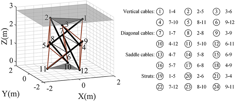
Figure 2. Shape-controlled double-layered tri-prism tensegrity structure.

TABLE 1

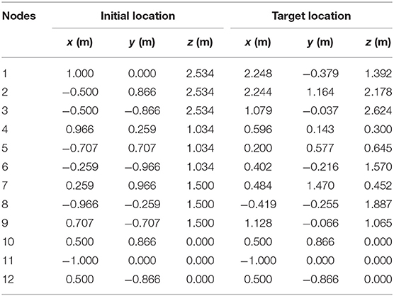
Table 1. Nodal coordinates of the double-layered tri-prism tensegrity system.

Properties of the members used for the shape-controlled tensegrity structure are given in Table 2. A fictitious nodal mass of 1.00 is assumed because the dynamics of the system was not considered in this shape control problem. A linear stiffness of 2 × 10⁵ N/m for struts and a linear stiffness of 200 N/m for cables are assumed. The “kinetic damping” is used to expedite the convergence of the DRM. The GA's parameters are set as follows: The population size is 50; the selection type is stochastic universal sampling; the crossover type is two-point; the crossover probability is 1; the mutation probability is 0.7 divided by bits of coding; the maximum number of generations is 200. The algorithm stops when the number of generations reach the maximum number specified.

TABLE 2

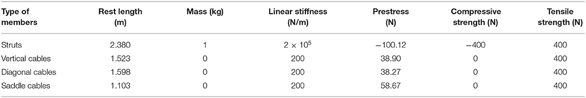
Table 2. Properties of members of the double-layered tri-prism tensegrity system.

Vertical and diagonal cables are used as active elements whose rest lengths can actively change in the ranges of 0.40–3.20 m and 0.05–4.00 m, respectively. The control strategy represented by the actuating function is simplified using the following approach: The actuating function for an active element is divided into a series of actuating steps; in each step the rest length of the active element is assumed to be linearly changed. Given the initial rest length, initial time, end time, and the rest length at the end of each step, the linear actuating function of the element in each step is easily determined. Denoting the rest length change of the element i in the k^th step as e_ik, the actuating function of an element with q steps can be expressed as e_i (e_i1, e_i2, …, e_iq). Further assuming that all the active elements possess the same division of actuating steps, i.e., all have q steps and the start time and end time of each step are the same for all active elements, the actuating function of the system can be expressed as Δ{e₁, e₂, …, e_nc}.

Path Optimization

The requirement to be collision-free is considered as an additional constraint, expressed as S ∈ Ω_c, in which S represents the state of the system and Ω_c represents the states without internal collision. The target state of the control is imposed as a further constraint that U^tf = U_target. The target state, i.e., the target location of nodes, is given in Table 1. This corresponds to change the center of the top triangle of the double-layered tensegrity from the initial position (0.000, 0.000, and 2.534) to (1.857, 0.249, and 2.065). The energy cost of the control strategy is used as the objective which can be expressed as:

$\begin{array}{ll}G(\Delta )={\displaystyle \sum _{t=t_s}^{t_f}}{\displaystyle \sum _{i=1}^{n_c}}\left|\frac{1}{2}(F_i^t+F_i^{t-\Delta t})(e_i^t-e_i^{t-\Delta t})\right|& (19)\end{array}$

where n_c is the number of elements; $F_i^t$ and $F_i^{t-\Delta t}$ are the internal forces of the i^th element at times t and t-Δt, respectively; and $e_i^t$ and $e_i^{t-\Delta t}$ are the rest length changes of the i^th element at times t and t-Δt, respectively. The control model is rewritten as

$\begin{array}{ll}\{\begin{array}{l}find\Delta \hfill \\ \min G\left(\Delta \right)={\displaystyle {\sum }_{t=t_s}^{t_f}{\displaystyle {\sum }_{i=1}^{n_c}\left|\frac{1}{2}(F_i^t+F_i^{t-\Delta t})(e_i^t-e_i^{t-\Delta t})\right|}}\hfill \\ s\text{.}t\text{.}\hfill \\ {\text{F}}_e^t-{\text{A}}^t{\text{F}}^t=\text{M}{\stackrel{\mathrm{..}}{\text{U}}}^t+\text{C}{\stackrel{.}{\text{U}}}^t\hfill \\ \Delta \in \text{E}\hfill \\ \text{U}\in {\Omega }_{\text{s}}\hfill \\ {\text{F}}^t\in {\Omega }_{\text{f}}\hfill \\ \text{S}\in {\Omega }_{\text{c}}\hfill \\ {\text{U}}^{t_f}={\text{U}}_{\text{target}}\hfill \end{array}& (20)\end{array}$

The reciprocal of the objective, i.e., 1/G(Δ), is selected as the fitness for the GA. The number of actuating steps is assumed to be 2, i.e., q = 2. The computation is carried out on a personal computer with a Intel Core i7-4790k CPU @ 4.0 GHz and 16 GB RAM. It has taken 293 min to carry out the 200-generation revolution. It is observed that the total energy assumption decreases rapidly in the first 46 generations and then converges slowly on 258.17 N·m (Figure 3). The optimal control strategy, corresponding to the minimum energy cost, is shown in Table 3, and the equilibrium configuration at the end of each actuating step of the optimal control strategy is shown in Figure 4. The motion trajectory of the center of upper triangle during the control is shown in Figure 5, in which the thick blue line represents the optimal path generated by the optimal control strategy, and the thin red lines represent 10 feasible paths generated by 10 feasible control strategies found in the evolution process. It is observed that the motion path generated by the optimal control strategy is much shorter than those generated by the unoptimized control strategies.

FIGURE 3

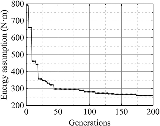
Figure 3. Total rest length change vs. generations.

TABLE 3

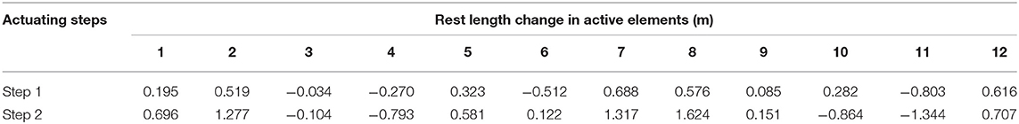
Table 3. Optimal control strategy for the double-layered tri-prism tensegrity structure.

FIGURE 4

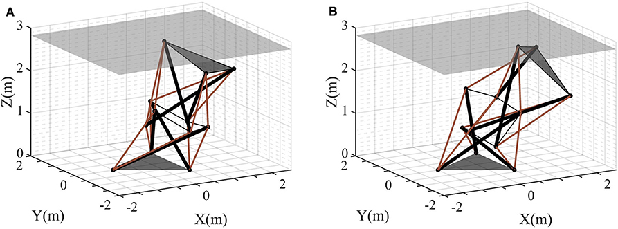
Figure 4. Equilibrium configuration after each actuating step: (A) after first step and (B) after second step.

FIGURE 5

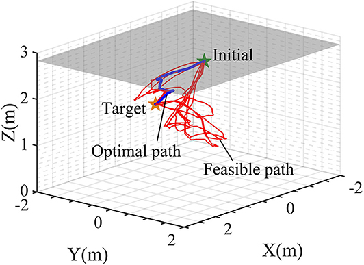
Figure 5. Motion path of the center of the upper triangle.

Locomotion Control

Locomotive Tensegrity System

The application of the proposed model and method to locomotion control in tensegrity systems is tested in a six-strut locomotive tensegrity structure. As shown in Figure 6, the tensegrity system comprises 12 nodes, 6 compression elements, and 24 tension elements. The connectivities and numbers of the elements are also shown in Figure 6. The 24 tension elements generate a pattern of 20 triangles on the outer surface of the structure. Eight of the surface triangles, each of which is closed by elements, are called closed triangles (TC). The other triangles are called opened triangles (TO) because each has only two tension elements and one edge of the triangle is open. For instance, as shown in Figure 6, the triangle with nodes 3, 7, and 12 is a TC, and the triangle with nodes 3, 11, and 12 is a TO. In the ideal state without external load and gravity, the compression elements and the tension elements have the same geometrical length. As a result, in the ideal state all the TCs and TOs are identical.

FIGURE 6

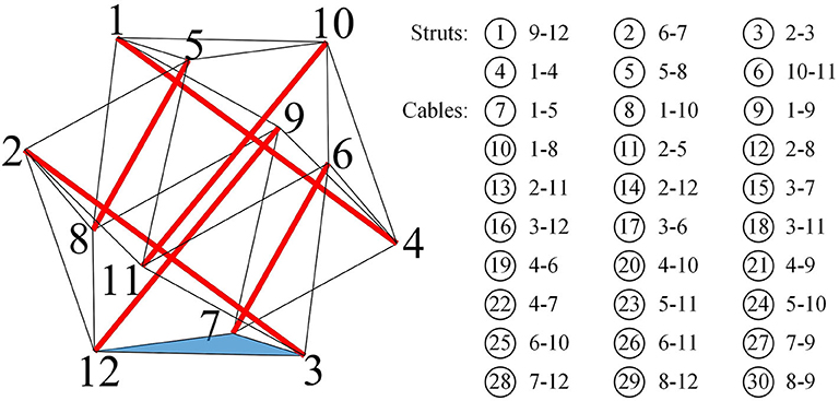
Figure 6. Six-strut tensegrity system.

The six compression elements are used as active elements, with an actuating range of [−5, 5] cm. The actuating speed is assumed to be 10 mm/s. The rest lengths of elements at the initial state and the mechanical properties of the elements are as shown in Table 4. The initial state of the system is obtained by applying gravity to the ideal state. A damping coefficient of 0.01 is assumed for the elements. Environmental parameters are set as follows: A stiffness of 1,000 N/m, and a friction coefficient of 0.5 are assumed for the ground; the gravitational acceleration is −9.8 m/s².

TABLE 4

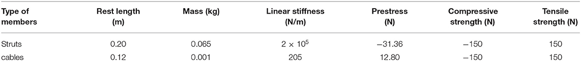
Table 4. Rest lengths at initial state and mechanical properties of elements.

Gait Design

The gait of the locomotive tensegrity structure is designed to satisfy the conditions that (1) the system acquires a certain amount of motion after the gait; and (2) the rest lengths of active elements are not changed before and after the gait, i.e.,

$\begin{array}{ll}{\Delta }^{t_f}={\Delta }^{t_s}& (21)\end{array}$

The motion of the system can be expressed by the displacement of the mass center as Δu^t_c = ||u^t_c-u^ts_c||, in which u_c = [u_cx, u_cy, u_cz] is the coordinate of the mass center.

Regarding the symmetry of the tensegrity system, there are two basic stand states in the locomotive system: the TC state and the TO state. As indicated by the names, the tensegrity structure stands on the ground with a TC in the TC state, and with a TO in the TO state.

There are two typical types of gaits for the six-strut locomotive tensegrity system, namely crawling gaits, and rolling gaits (Li et al., 2017). It can be easily recognized that rolling gaits usually generate a larger motion than crawling gaits. To obtain rolling gaits rather than crawling gaits, the objective function for gait design is defined to maximize the horizontal motion of the mass center of the system, i.e.,

$\begin{array}{ll}G(\Delta )=\frac{1}{\Delta u_{cxy}^{t_f}+1},\Delta u_{cxy}^{t_f}=\sqrt{{\left(u_{cx}^{t_f}-u_{cx}^{t_s}\right)}^2+{\left(u_{cy}^{t_f}-u_{cy}^{t_s}\right)}^2}& (22)\end{array}$

where ${\Delta u}_{cxy}^{t_f}$ is the horizontal motion distance of the mass center at time t_f; $u_{cx}^{t_s}$ and $u_{cy}^{t_s}$ are the x and y coordinates of the mass center at time t_s; and $u_{cx}^{t_f}$ and $u_{cy}^{t_f}$ are the x and y coordinates of the mass center at time t_f. An additional constraint on the number of active elements used in the gait is adopted to impose control on the number of active elements used in the motion. The additional constraint is written as

$\begin{array}{ll}{n}_a=N_a& (23)\end{array}$

where n_a is the number of active elements used in the gait, and N_a is an integer constant no larger than 6, specified by the designer.

Substituting the above objective in Equation (22) and additional constraints Equations (21) and (23) into Equation (12), an optimization model for the gait design can be obtained:

$\begin{array}{ll}\{\begin{array}{l}find\Delta \hfill \\ \min G\left(\Delta \right)=\frac{1}{\Delta u_{cxy}^{t_f}+1}\hfill \\ s\text{.}t\text{.}\hfill \\ {\text{F}}_e^t-{\text{A}}^t{\text{F}}^t=\text{M}{\stackrel{\mathrm{..}}{\text{U}}}^t+\text{C}{\stackrel{.}{\text{U}}}^t\hfill \\ \Delta \in \text{E}\hfill \\ \text{U}\in {\Omega }_{\text{s}}\hfill \\ {\text{F}}^t\in {\Omega }_{\text{f}}\hfill \\ {\Delta }^{t_f}={\Delta }^{t_s}\hfill \\ n_a=N_a\hfill \end{array}& (24)\end{array}$

The method proposed in this paper is used to solve this model. The GA used here adopts a maximum number of generations of 100, and the other parameters of it are same as those used in section Shape Control. The computations are carried out with the same computer used in section Shape Control. Two cases, using the TC state and TO state, as the initial state, are considered. The number of stand triangles and triangles adjacent to the stand triangle are shown in Figure 7. In each case, six computations, corresponding to N_a = 1, 2, 3, 4, 5, and 6, are performed. The evolution process of the mass center's horizontal motion distance in the computations are shown in Figure 8. In the case using the TC state as the initial state, three typical gaits that, respectively, drive the system rolling from the current stand triangle to the three adjacent triangles are found (Table 5). The motion distance of the mass center generated by these gaits is in the range 6.40–6.50 cm. In the case using the TO state as the initial state, there are also three gait types. Two respectively, drive the system rolling from the initial stand triangle to two of the three adjacent triangles, whereas the third drives the system rolling twice, from the initial stand triangle to an adjacent triangle, and then to an adjacent triangle again (Table 5). The motion distance of the mass center generated by the single-rolling gaits is 6.24 cm. The motion distance of the mass center generated by the double-rolling gait is 10.48 cm; about 1.68 times that generated by the single-rolling gaits.

FIGURE 7

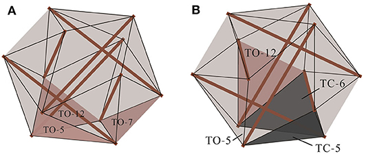
Figure 7. Two initial states: (A) TC state and (B) TO state.

FIGURE 8

Figure 8. Motion distance vs. generations: (A) TC state and (B) TO state.

TABLE 5

Table 5. Locomotive gait for the six-strut tensegrity structure.

Motion Path Planning

For a given initial and target location pairing, there are generally two approaches to realizing motion from the initial to the target location. One is connecting the initial location to the target location using several basic gaits, as given in Table 5. This approach is suitable for regular movement on flat terrains with given maps, and a geometry-based algorithm has previously been verified for finding the path for locomotion of a six-strut tensegrity robot (Lu et al., 2019). The other approach is a direct search for a control strategy able to drive movement of the system from the initial location to the target location. This approach is considered more flexible than the first, but normally carries greater computational cost because it has to numerically track motion within the path planning scheme. In the current work, the second approach is adopted. The locations A(x_A, y_A) and B(x_B, y_B) are defined as the initial location and the target location.

The objective function is defined as:

$\begin{array}{ll}G(\Delta )=\{\begin{array}{c}d,ifd>\epsilon \\ 0,ifd\le \epsilon \end{array}& (25)\end{array}$

where d is the distance between the current location and the target location, and ε is a positive small constant.

The aforementioned additional constraint of no internal collision is included. The motion path planning model can thus be written as

$\begin{array}{ll}\{\begin{array}{l}find\Delta \hfill \\ \min G\left(\Delta \right)=\{\begin{array}{l}d,ifd>\epsilon \hfill \\ 0,ifd\le \epsilon \hfill \end{array}\hfill \\ s\text{.}t\text{.}\hfill \\ {\text{F}}_e^t-{\text{A}}^t{\text{F}}^t=\text{M}{\stackrel{\mathrm{..}}{\text{U}}}^t+\text{C}{\stackrel{.}{\text{U}}}^t\hfill \\ \Delta \in \text{E}\hfill \\ \text{U}\in {\Omega }_{\text{s}}\hfill \\ {\text{F}}^t\in {\Omega }_{\text{f}}\hfill \\ {\Delta }^{t_f}={\Delta }^{t_s}\hfill \end{array}& (26)\end{array}$

The initial location is set as A (0, 0) and the target location as B (0.1, 0.1). The starting time is set as t_s = 0, the end time as t_f = 150 s, and the positive small constant ε as 0.0005 m. Time is discretized by an interval of 1 s. The GA used here adopts the same set of parameters as used in section Gait Design. It has taken 1,750 min to complete 75 generations on the same computer as that used for the motion path planning optimization.

The evolution of the average and minimum objectives in the computation is shown in Figure 9. The minimum distance between the current and the target location decreases to 0.0004 m in the 69th generation. The individual corresponding to the minimum objective in the last generation is the optimal control strategy, represented by the rest length change spectra of the six active elements, as shown in Figure 10A. The motion trajectory of the system's mass center under the optimal control strategy is shown in Figure 10B. Further investigation into the motion reveals that the system experiences three complete rolls and the stand triangle shifts from TC-6 (3, 7, 12) to TO-7 (3, 4, 7), TC-8 (4, 7, 9), and finally TO-11 (7, 8, 9). Besides the rolling movements, some crawls and shape adjustments occurs, resulting in small-scale movements, as indicated by the red dashed-line rectangles in Figure 10B.

FIGURE 9

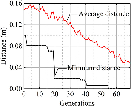
Figure 9. Evolution process of motion path planning.

FIGURE 10

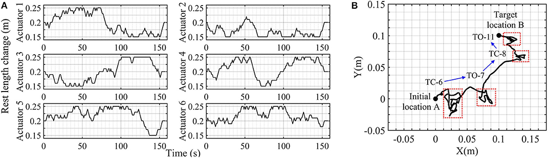
Figure 10. Optimal solution: (A) control strategy and (B) motion path.

Discussion

In this paper, the generality of the proposed model is ensured by the following factors: It does not deliberately distinguish between the shape-controlled tensegrity structure and the locomotive tensegrity structure. A unified dynamic formulation is used for the controllable tensegrity structure, though the shape control process is usually deemed to be quasi-static. The DRM-based algorithm using the central difference explicit scheme can track both the deformations and global rigid body motions of tensegrity systems. Conceptual expressions of the subjective and constraints were adopted. The control problem for a controllable tensegrity structure was interpreted as a combinational optimization problem. A similar optimization model was used for shape-controlled tensegrity structures in previous studies (Xu and Luo, 2009; Xu et al., 2014). However, in the current work, quasi-static behavior was assumed for the structural system, and the global rigid body motion of the structural system was eliminated by proper restraints. To some extent, the proposed model may be considered an extension of the previous model.

The global optimization algorithm used in the paper, i.e., the GA, worked well in the shape control example in section Shape Control and the locomotion control example in section Locomotion Control. In both examples, the number of control steps was provided in advance. Situations in which the number of control steps cannot be determined in advance, as in the path planning situations considered in the literature (Xu et al., 2014; Lu et al., 2019), are difficult to handle with a GA. Further considering that there is no constraint on the number of control steps in the mathematical model given in Equation (12), the generality of the GA does not match that of the model. Various other global optimization algorithms besides a GA could be used, based on the specific application.

Conclusion

In this paper, a general model for both shape control and locomotion control of tensegrity systems is proposed. A method combining GA and DRM was adopted to solve the model. The proposed model and method were applied to typical tensegrity system shape and locomotion control problems. The results demonstrate that both the shape control problem of a double-layered tri-prism tensegrity structure, and the locomotion control problem of a six-strut tensegrity structure can be modeled by the proposed model, and solved by the proposed method. We believe the proposed model is also suitable for control problems in other types of tensegrity system. The applicability of the proposed GA-based method to control problems of higher complexity and larger scale than those presented in this work could be subject of future investigation.

Data Availability Statement

All datasets generated for this study are included in the article/supplementary material.

Author Contributions

HC developed the model and method for the controllable tensegrity. XX proposed the main idea of the paper. MW assisted HC in the numerical computations in the applications. YL developed the DRM-based algorithm for dynamic tensegrity. All authors contributed to the article and approved the submitted version.

Funding

This work was supported by the Natural Science Foundation of Zhejiang Province (LR17E080001) and the Natural Science Foundation of China (51578494).

Conflict of Interest

The authors declare that the research was conducted in the absence of any commercial or financial relationships that could be construed as a potential conflict of interest.

References

Al Sabouni-Zawadzka, A. (2014). Active control of smart tensegrity structures. Arch. Civil Eng. 60, 517–534. doi: 10.2478/ace-2014-0034

CrossRef Full Text | Google Scholar

Amendola, A., Krushynska, A., Daraio, C., Pugno, N. M., and Fraternali, F. (2018). Tuning frequency band gaps of tensegrity mass-spring chains with local and global prestress. Int. J. Solids Struct. 155, 47–56. doi: 10.1016/j.ijsolstr.2018.07.002

CrossRef Full Text | Google Scholar

Barnes, M. R. (1999). Form finding and analysis of tension structures by dynamic relaxation. Int. J. Space Struct. 14, 89–104. doi: 10.1260/0266351991494722

CrossRef Full Text | Google Scholar

Bliss, T., Iwasaki, T., and Bart-Smith, H. (2013). Central pattern generator control of a tensegrity swimmer. IEEE/ASME Trans. Mech. 18, 586–597. doi: 10.1109/TMECH.2012.2210905

CrossRef Full Text | Google Scholar

Böhm, V., and Zimmermann, K. (2013). “Vibration-driven mobile robots based on single actuated tensegrity structures,” in Proceedings - IEEE International Conference on Robotics and Automation. (Karlsruhe), doi: 10.1109/ICRA.2013.6631362

CrossRef Full Text | Google Scholar

Cera, B., and Agogino, A. M. (2018). “Multi-cable rolling locomotion with spherical tensegrities using model predictive control and deep learning,” in: IEEE International Conference on Intelligent Robots and Systems (Madrid), 6595–6600. doi: 10.1109/IROS.2018.8594401

CrossRef Full Text | Google Scholar

Fazli, N., and Abedian, A. (2011). Design of tensegrity structures for supporting deployable mesh antennas. Scientia Iranica 18, 1078–1087. doi: 10.1016/j.scient.2011.08.006

CrossRef Full Text | Google Scholar

Fest, E., Shea, K., Domer, B, and Smith, I. F. C. (2003). Adjustable tensegrity structures. J. Struct. Eng. 129, 515–526. doi: 10.1061/(ASCE)0733-9445(2003)129:4(515)

CrossRef Full Text | Google Scholar

Fraternali, F., Carpentieri, G., Amendola, A., Skelton, R. E., and Nesterenko, V. F. (2014). Multiscale tunability of solitary wave dynamics in tensegrity metamaterials. Appl. Phys. Lett. 105:201903. doi: 10.1063/1.4902071

CrossRef Full Text | Google Scholar

Friesen, J., Pogue, A., Bewley, T., Oliveira, M. D., Skelton, R., and Sunspiral, V. (2014). “DuCTT: a tensegrity robot for exploring duct systems,” in Proceedings - IEEE International Conference on Robotics and Automation (Hong Kong), 4222–4228. doi: 10.1109/ICRA.2014.6907473

CrossRef Full Text | Google Scholar

Friesen, J. M., Glick, P., Fanton, M., Manovi, P., and Sunspiral, V. (2016). “The second generation prototype of a duct climbing tensegrity robot, DuCTTv2,” in Proceedings - IEEE International Conference on Robotics and Automation (Stockholm), 2123–2128. doi: 10.1109/ICRA.2016.7487361

CrossRef Full Text | Google Scholar

Kan, Z., Peng, H., Chen, B., and Zhong, W. (2018). Nonlinear dynamic and deployment analysis of clustered tensegrity structures using a positional formulation FEM. Compos. Struct. 187, 241–258. doi: 10.1016/j.compstruct.2017.12.050

CrossRef Full Text | Google Scholar

Khazanov, M., Humphreys, B., Keat, W., and Rieffel, J. (2013). “Exploiting dynamical complexity in a physical tensegrity robot to achieve locomotion,” in The Twelfth European Conference on Artificial Life (East Lansing, MI), 965–972. doi: 10.7551/978-0-262-31709-2-ch144

CrossRef Full Text | Google Scholar

Kim, K. (2016). On the locomotion of spherical tensegrity robots (PhD dissertation). University of California, Berkeley, CA, United States.

PubMed Abstract | Google Scholar

Kim, K., Moon, D., Bin, J. Y., and Agogino, A. M. (2017). “Design of a spherical tensegrity robot for dynamic locomotion,” in IEEE International Conference on Intelligent Robots and Systems (Vancouver, BC), 450–455. doi: 10.1109/IROS.2017.8202192

PubMed Abstract | CrossRef Full Text | Google Scholar

Li, B., Du, W., and Liu, W. (2017). “Dynamic modeling and controlling for the crawling motion of the 6-strut tensegrity robot,” in 2017 IEEE 7th Annual International Conference on CYBER Technology in Automation, Control, and Intelligent Systems (CYBER) (Honolulu, HI: IEEE). doi: 10.1109/CYBER.2017.8446093

CrossRef Full Text | Google Scholar

Lin, C., Li, D., and Zhao, Y. (2016). “Tensegrity robot dynamic simulation and kinetic strategy programming,” in 2016 IEEE Chinese Guidance, Navigation and Control Conference (CGNCC) (Nanjing), 2394–2398.

Google Scholar

Liu, K., Zegard, T., Pratapa, P. P., and Paulino, G. H. (2019). Unraveling tensegrity tessellations for metamaterials with tunable stiffness and bandgaps. J. Mech. Phys. Solids 131, 147–166. doi: 10.1016/j.jmps.2019.05.006

CrossRef Full Text | Google Scholar

Lu, Y., Xu, X., and Luo, Y. (2019). Path planning for rolling locomotion of polyhedral tensegrity robots based on Dijkstra algorithm. J. Int. Assoc. Shell Spatial Struct. 60, 271–284. doi: 10.20898/j.iass.2019.202.037

CrossRef Full Text | Google Scholar

Luo, A., and Liu, H. (2017). Analysis for feasibility of the method for bars driving the ball tensegrity robot. J. Mech. Robotics 9:051010. doi: 10.1115/1.4037565

CrossRef Full Text | Google Scholar

Mirletz, B. T., Bhandal, P., Adams, R. D., Agogino, A. K., Quinn, R. D., and SunSpiral, V. (2015). Goal-directed CPG-based control for tensegrity spines with many degrees of freedom traversing irregular terrain. Soft Robotics 2, 165–176. doi: 10.1089/soro.2015.0012

CrossRef Full Text | Google Scholar

Motro, R. (2003). Tensegrity: Structural Systems for the Future. London: Kogan Page Science. doi: 10.1016/B978-190399637-9/50038-X

CrossRef Full Text | Google Scholar

Oden, J. T., and Kikuchi, N. (1982). Finite element methods for constrained problems in elasticity. Int. J. Numerical Methods Eng. 18, 701–725. doi: 10.1002/nme.1620180507

CrossRef Full Text | Google Scholar

Oh, C. L., Choong, K. K., Nishimura, T., Kim, J. Y., and Zain, M. R. (2018). Tapered three-stage deployable tensegrity model. J. Phys. Conf. Ser. 1130:012031. doi: 10.1088/1742-6596/1130/1/012031

CrossRef Full Text | Google Scholar

Omer, O., Offer, S., Amir, A., and Uri, B. -,H. (2011). “A model of caterpillar locomotion based on assur tensegrity structures,” in ASME 2011 International Design Engineering Technical Conferences and Computers and Information in Engineering Conference (Washington, DC).

Google Scholar

Papadopoulos, P., and Taylor, R. L. (1992). A mixed formulation for the finite element solution of contact problems. Comput. Methods Appl. Mech. Eng. 94, 373–389. doi: 10.1016/0045-7825(92)90061-N

CrossRef Full Text | Google Scholar

Park, S., Park, E., Yim, M., Kim, J., and Seo, T. (2019). Optimization-based nonimpact rolling locomotion of a variable geometry truss. IEEE Robotics Automation Lett. 4, 747–752. doi: 10.1109/LRA.2019.2892596

CrossRef Full Text | Google Scholar

Paul, C., Valero-Cuevas, F. J., and Lipson, H. (2006). Design and control of tensegrity robots for locomotion. IEEE Trans. Robotics 22, 944–957. doi: 10.1109/TRO.2006.878980

CrossRef Full Text | Google Scholar

Rovira, A. G., and Tur, J. M. M. (2009). Control and simulation of a tensegrity-based mobile robot. Robotics Auton. Syst. 57, 526–535. doi: 10.1016/j.robot.2008.10.010

CrossRef Full Text | Google Scholar

Sabelhaus, A. P., Bruce, J., Caluwaerts, K., Manovi, P., and Sunspiral, V. (2015). System design and locomotion of SUPERball, an untethered tensegrity robot,” in Proceedings - IEEE International Conference on Robotics and Automation (Seattle, WA), 2867–2873. doi: 10.1109/ICRA.2015.7139590

CrossRef Full Text | Google Scholar

Senatore, G., and Piker, D. (2015). Interactive real-time physics: an intuitive approach to form-finding and structural analysis for design and education. Comput. Aided Design 61, 32–41. doi: 10.1016/j.cad.2014.02.007

CrossRef Full Text | Google Scholar

Shea, K., Fest, E., and Smith, I. F. C. (2002). Developing intelligent tensegrity structures with stochastic search. Adv. Eng. Inform. 16, 21–40. doi: 10.1016/S1474-0346(02)00003-4

CrossRef Full Text | Google Scholar

Sultan, C., Corless, M., and Skelton, R. E. (2002). Symmetrical reconfiguration of tensegrity structures. Int. J. Solids Struct. 39, 2215–2234. doi: 10.1016/S0020-7683(02)00100-2

CrossRef Full Text | Google Scholar

Sultan, C., and Skelton, R. (2003). Deployment of tensegrity structures. Int. J. Solids Struct. 40, 4637–4657. doi: 10.1016/S0020-7683(03)00267-1

CrossRef Full Text | Google Scholar

SunSpiral, V., Gorospe, G., Bruce, J., Iscen, A., Korbel, G., Milam, S., et al. (2013). “Tensegrity based probes for planetary exploration entry, descent and landing (EDL) and surface mobility analysis,” in Proceedings of 10th International Planetary Probe Workshop (San Jose, CA).

Google Scholar

Veuve, N., Safaei, S. D., and Smith, I. F. C. (2015). Deployment of a tensegrity footbridge. J. Struct. Eng. 141:04015021. doi: 10.1061/(ASCE)ST.1943-541X.0001260

CrossRef Full Text | Google Scholar

Wang, Z., Li, K., He, Q., and Cai, S. (2019). A light-powered ultralight tensegrity robot with high deformability and load capacity. Adv. Mater. 31:1806849. doi: 10.1002/adma.201806849

PubMed Abstract | CrossRef Full Text | Google Scholar

Xu, X., and Luo, Y. (2009). Non-linear displacement control of prestressed cable structures. Proc. Inst. Mech. Eng. Part G: J. Aerospace Eng. 223, 1001–1007. doi: 10.1243/09544100JAERO455

CrossRef Full Text | Google Scholar

Xu, X., and Luo, Y. (2013). Collision-free shape control of a plane tensegrity structure using an incremental dynamic relaxation method and a trial-and-error process. Proc. Inst. Mech. Eng. Part G: J. Aerospace Eng. 227, 266–272. doi: 10.1177/0954410011433501

CrossRef Full Text | Google Scholar

Xu, X., Sun, F., Luo, Y., and Xu, Y. (2014). Collision-free path planning of tensegrity structures. J. Struct. Eng. 140:04013084. doi: 10.1061/(ASCE)ST.1943-541X.0000900

CrossRef Full Text | Google Scholar

Yu, Y., and Luo, Y. (2009). Finite particle method for kinematically indeterminate bar assemblies. J. Zhejiang Univ. Sci. A 10, 669–676. doi: 10.1631/jzus.A0820494

CrossRef Full Text | Google Scholar

Yu, Y., Paulino, G. H., and Luo, Y. (2011). Finite particle method for progressive failure simulation of truss structures. J. Struct. Eng. 137, 1168–1181. doi: 10.1061/(ASCE)ST.1943-541X.0000321

CrossRef Full Text | Google Scholar

Zhang, L., Maurin, B., and Motro, R. (2006). Form-finding of nonregular tensegrity systems. J. Struct. Eng. 132, 1435–1440. doi: 10.1061/(ASCE)0733-9445(2006)132:9(1435)

CrossRef Full Text | Google Scholar

Zhao, Y., Zhou, S., Lin, C., and Li, D. (2017). “An efficient locomotion strategy for six-strut tensegrity robots,” in 2017 13th IEEE International Conference on Control & Automation (ICCA) (Ohrid). doi: 10.1109/ICCA.2017.8003096

CrossRef Full Text | Google Scholar