Investigation of Hybrid Simulation With Model Updating Compared to an Experimental Shake Table Test

1. Introduction

Hybrid simulation was initially introduced by Hakuno et al. (1969) and Mahin and Shing (1985) and is typically viewed as a cost-effective method for dynamic analysis of infrastructures. In a hybrid simulation, structural components are (1) expected to experience significant nonlinearity or (2) difficult to model accurately and are thus tested physically and are known as the experimental substructure. The rest of the structure is included in a numerical model, denoted by the numerical substructure. The experimental and numerical substructures are coupled at each of the boundaries through loading devices. These loading devices, such as hydraulic actuators, electric motors, and shake tables, etc., apply the calculated responses (normally a displacement) at the boundary to the physical specimen. The responses of the physical specimens are then measured accordingly and sent back to the numerical model, as in Phillips and Spencer (2012) and Ou et al. (2015). The responses of the entire structure, including story drifts, displacements, and accelerations, can be monitored during the test. Therefore, this testing method can evaluate global structural performance. For the experimental substructure to be tested physically, its local behaviors, including crack initialization, material, and geometric nonlinearity evolution under loading, and even failure modes, can also be investigated during testing (Gomez et al., 2014). Therefore, hybrid simulation is known to preserve both global and local observations for structural performance assessment.

In the previous applications, hybrid simulation has shown great advantages in studying local and global performance of structural vibration control devices (Christenson et al., 2008; Karavasilis et al., 2011; Lin et al., 2012; Gao et al., 2013). Due to the isolated and critical role of these devices and components, it was intuitive to select them as the experimental substructure. New advances have taken place in the infrastructural system and component design, such as shear walls and rocking frames, distributed structural fuses, etc., and their behaviors are also to be studied. These components, with their appearance patterns repetitively and spatially distributed among the entire structure design, do not have a substantially different role between one component to the other (Elnashai et al., 2008). To investigate their performance in a hybrid simulation setup, a couple of challenges need to be addressed. Due to the more equally weighted contribution of these components to the structure level performance, it is difficult to select the experimental substructure among their multiple use. Meanwhile, the facility capacity (number of actuators and lab space), available budget, and the number of the experimental substructure are limited. As a result, for hybrid simulation to be applied in these cases, a larger portion of the target components must still reside in the numerical substructure. Therefore, the hybrid simulation fidelity is affected by modeling accuracy of numerical components rather than the response of their physical counterparts. Two questions were posed in Kwon and Kammula (2013): (1) Out of many similar structural elements, which elements should be experimentally represented? (2) How much increase in accuracy can be achieved by physically modeling only a few elements?

To address such challenges, a new branch of hybrid simulation has been established recently, known as hybrid simulation with model updating (HSMU). In HSMU, hybrid simulation is integrated with on-line system identification methods. Here, the input and response histories measured from the physical specimen are used in an online identification module to estimate model parameters that best represent the physical specimen. The identified model is then used to update the portions of the numerical model that are associated with the counterparts to that physical specimen. Several researchers have concluded that using model updating in a hybrid simulation yields large improvements in the results (for instance Hashemi et al., 2014; Wu and Wang, 2015; Elanwar and Elnashai, 2016; Shao et al., 2016; Ou et al., 2017). The fidelity of HSMU is commonly assessed to be evaluating the model identification accuracy and the convergence of model parameters which can be only a local optimal criterion. Ou and Dyke (2016) further demonstrated the improvement of fidelity assessment with additional verification tests after an HSMU. In the validation stage, a new specimen representing one numerical counterpart in the HSMU was loaded with its displacement trajectory and experienced numerically in the HSMU. Later, the measured force response was compared to the calculated response (force) in the HSMU with the model parameter updated in real time.

In the state-of-the-art study, the HSMU used the following assumptions: the model updating method is adaptive to the ground motion and can identify a converged set of numerical parameters of the model; and the local performance assessment can indicate the fidelity of the HSMU. In this paper, we present the investigation of the two assumptions and studied the improvements in model fidelity while using HSMU with two models. The experimental HSMU responses of a five-story frame with identical floors are examined; the frame is expected to develop distributed nonlinearity across several floors. Time response analysis is performed using (1) conventional simulation, (2) HSMU, and (3) shake table testing. The first story is selected as the experimental substructure while the upper stories are included in the computational substructure. The parameters of the model of the experimental substructure are identified during testing and used to update the numerical substructure. In case I, each frame (each floor) is modeled with a concentrated nonlinear Bouc-Wen model in a lumped mass system. In case II, a fiber model with material nonlinearity is used as the nonlinear model to be identified, and the material properties are identified using measured responses. The improvements in the accuracy of the results are investigated at both the local and global level. Local assessment of HSMU performance focuses on the accuracy and efficiency of the model updating, and the parameters' adaptiveness using ground motions with different magnitude. Global performance is assessed through a direct comparison of the responses with pure simulation and shake table results. Conclusions will be addressed from the point of view of both the time and frequency domain analyses.

2. HSMU Formulation and Implementation

In a conventional simulation, the dynamic response of the whole structure is represented by the equation of motion:

$\begin{array}{ll}Mẍ+Cẋ+F(x,ẋ)+R(x,ẋ,{\theta }_R)=-M\Gamma {ẍ}_g& (1)\end{array}$

where, ẍ_g is the ground motion; M, C, and K are the mass, damping, and stiffness matrices of the master structure, respectively; R is the nonlinear restoring force; and θ_R is the parameter set governs the nonlinear behavior of the structure.

In a hybrid simulation, the structure is partitioned, and the associated equations of motion then take the form

$\begin{array}{ll}{M}^N{ẍ}^N+C^N{ẋ}^N+F^E(x^E,{ẋ}^E)+R^N(x^N,{ẋ}^N,{\theta }_R)=-M\Gamma {ẍ}_g& (2)\end{array}$

$\begin{array}{ll}{M}^E{ẍ}^E+C^E{ẋ}^E+R^E(x^E,{ẋ}^E)=F^E(x^E,{ẋ}^E)& (3)\end{array}$

where, the superscripts ()^N and ()^E denote the portions of the structure that reside in the numerical substructure and experimental substructures. Here, M = M^E + M^N, C = C^E + C^N, K = K^E + K^N, and F^E is the force measured from the experimental substructure. When the physical specimen is selected to be a structural component that is used repeatedly in multiple instances within the master structure, a limited number of substructures are selected for physical experimentation. Thus, a significant portion of their counterparts reside in the numerical substructure (R^N >> R^E) and have similar behavior. When the numerical model is unknown, and thus potentially inaccurate (either the type of model or model parameters), modeling errors present in R^N may dominate the source of errors of the hybrid simulation.

To reduce the modeling errors in the numerical substructure, hybrid simulation is enhanced by incorporating model updating. Thus, the equations of motion become:

$\begin{array}{ll}{M}^N{ẍ}^N+C^N{ẋ}^N+K^N{x}^N+F^E(x^E,{ẋ}^E)+R^N(x^N,{ẋ}^N,{\tilde{\theta }}_R)=-M\Gamma {ẍ}_g& (4)\end{array}$

$\begin{array}{ll}{M}^E{ẍ}^E+C^E{ẋ}^E+K^E{x}^E+R^E(x^E,{ẋ}^E)=F^E(x^E,{ẋ}^E)& (5)\end{array}$

$\begin{array}{ll}{\tilde{\theta }}_R=\text{Ψ}(R^E,x^E,{ẋ}^E,{\theta }_{\text{Ψ}})& (6)\end{array}$

where Ψ is the model-updating module used in the HSMU, which is executed in real time, and ${\tilde{\theta }}_R$ is the recursively identified nonlinear model parameters that minimize an associated cost function. Therefore, with the nonlinear restoring parameter set ${\tilde{\theta }}_R$ updated according to the numerical substructure response in Equation (4), the numerical restoring force $R^N(x^N,{ẋ}^N,{\tilde{\theta }}_R)$ is assumed to have been updated to the experimental nonlinear behavior.

The constrained unscented Kalman filter (CUKF) was developed based on the unscented Kalman Filter and is selected as the model updating algorithm in this study. For structural analysis, it is common for the model parameters to have physical meanings, and many of these parameters fall within a certain range. CUKF allows a constrained projection on the state estimation for the unscented Kalman Filter, as presented by Kandepu et al. (2008).

The execution of CUKF in hybrid simulation is formulated as shown in Figure 1. The input space of the model is the displacement measured in the experimental substructure, and the output space is the experimental nonlinear restoring force. Ψ_ICUT indicates the interval constrained unscented transformation, γ is a coefficient set with γ_j associated with the jth transformed sigma points χ (total number of sigma points is 2L + 1), where L is the number of parameters to be updated. d and e are the lower and upper bounds for the model parameters. h() is the model function which takes each sigma point and projects it to the output space. P^XX, P^XY, and P^YY are the variance and co-variance matrices during state estimation. A detailed derivation of the formulation can be found in Ou et al. (2017).

FIGURE 1

Figure 1. Model updating as implemented in hybrid simulation platform.

3. Experimental Setup and Substructuring for Hybrid Simulation

In this study, nonlinear seismic responses of a five-story steel frame is investigated. Each story in the frame is identical, and the drawing of a typical story is shown in Figure 2A. Based on previous research and experiments (Song and Dyke, 2013), this structure behaves like a shear frame, and the use of this frame as the target structure enables a comparison of the results of hybrid simulation to shake table tests.

FIGURE 2

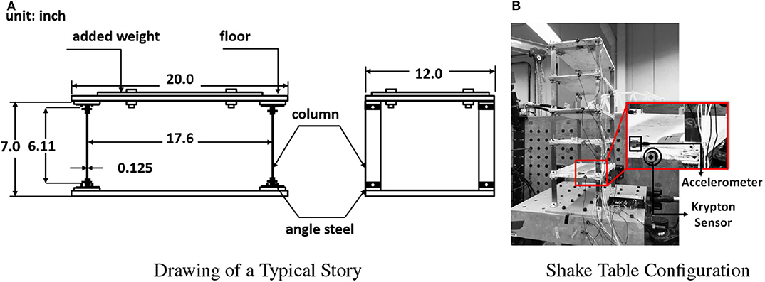
Figure 2. Specimen drawing and experimental setup. (A) Drawing of a typical story. (B) Shake table configuration.

For the shake table testing, the entire structure is mounted on a 6 DOFs shake table in the Intelligent Infrastructure System Lab (https://engineering.purdue.edu/IISL/) at Purdue University. The shake table is driven by six hydraulic actuators: two in the x-axis, one in the y-axis, and three in the z-axis. All actuators are controlled in the integrated SW6000 controller made by Shore Western. In this study, the ground motion is imposed only in the y axis. During the shake table tests, absolute acceleration and displacement responses of the frame are measured using accelerometers and optical sensors, as indicated in Figure 2B. VibPilot, a high resolution DAQ system, is used to record the structural acceleration response with a sampling frequency of 2,048 Hz, embedded anti-aliasing filters are applied during data acquisition. A 6D Krypton optical tracking system is used to measure the position of LED sensors placed on each floor which captures the 6D position and dynamic movement of each LED. The sampling rate of the Krypton system is set at 60 Hz.

The El Centro earthquake record is used as the ground motion for the structure. The earthquake is imposed twice sequentially, with an increasing magnitude to generate different level of nonlinearity. The ground motion is also condensed in time (using a reduction factor of 2) to develop nonlinear behavior in the structure while compensate the limitation of the maximum stroke to be applied to the shake table actuator. The entire excitation lasts 40 s. In the first 20 s (section 1, denoted as S1), the peak acceleration is 6.98 m/s², and in the later 20 s (section 2, denoted as S2), the acceleration reaches a peak of 18.3 m/s². The desired ground motion is shown in Figure 3A, and the measured shake table acceleration (as discussed later in Figure 6) is used as the excitation input in HSMUs and numerical simulations.

FIGURE 3

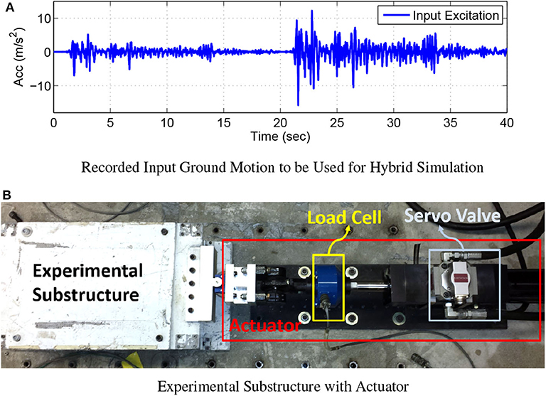
Figure 3. Testing ground motion and experimental substructure setup. (A) Recorded input ground motion to be used for hybrid simulation. (B) Experimental substructure with actuator.

For HSMU, the frame is partitioned into an experimental substructure (the first floor) and a numerical substructure (the remaining upper floors). The experimental substructure is attached to a Shore Western 1 kip hydraulic actuator as in Figure 3B. The SW6000 provides a PID loop for stabilization and inner loop control of the hydraulic actuator. Communication between the numerical substructure and experimental substructure is achieved using National Instruments (NI) hardware and LabVIEW software. During each computational time interval, the LabVIEW program receives the displacement command from the numerical solver and converts it into an analog signal to send to the SW6000 input. Note that, after each test, either in the case of a hybrid simulation or a shake table test, all columns with any evidence of yielding are replaced with new ones. All columns used in this study were cut from the same batch of steel to provide behavior that is quite similar. Therefore, the difference in the initial condition of the structure for each test is assumed to be negligible.

Two cases of HSMUs are conducted in this study. In case I, specimen nonlinearity is modeled with a Bouc-Wen-Baber-Noori model proposed by Baber and Wen (1981) and Baber and Noori (1985). In case II, the specimen nonlinearity in the numerical substructure is modeled with the constitutive steel model in OpenSees. Detailed explanations of each case are described in sections 3.1 and 3.2, respectively.

3.1. HSMU Case I: Bouc-Wen Model

In case I, the nonlinear behavior of the single-story frame is modeled with the phenomenological Bouc-Wen-Baber-Noori model. This model can capture the pinching and degradation effects in a structural component, represented by Equations (7)–(16).

$\begin{array}{ll}R(x^E,z)=\alpha k{x}^E+(1-\alpha )kz& (7)\end{array}$

$\begin{array}{ll}\dot{z}=h(z)\{\frac{{\dot{x}}^E-\nu (\epsilon )(\beta |{\dot{x}}^E||z{|}^{n-1}z+\gamma {\dot{x}}^E|z{|}^n}{\eta (\epsilon )}\}& (8)\end{array}$

where k is the stiffness coefficient, and 0 ≤ α ≤ 1 determines the level of nonlinearity. α = 1 indicates the system is purely linear and α = 1 indicates the system is purely hysteretic. The energy dissipation is represented by E(t):

$\begin{array}{ll}E(t)={\displaystyle \int }(1-\alpha )kz{ẋ}^{E}dt& (9)\end{array}$

$\begin{array}{ll}\epsilon (t)={\displaystyle \int }z{ẋ}^{E}dt& (10)\end{array}$

ν(ε) and η(ε) are degradation shape functions, and δ_ν, δ_η are degradation parameters.

$\begin{array}{ll}\nu (\epsilon )=1+{\delta }_{\nu }\epsilon & (11)\end{array}$

$\begin{array}{ll}\eta (\epsilon )=1+{\delta }_{\eta }\epsilon & (12)\end{array}$

A function h(z) describes the pinching effect is given by:

$\begin{array}{ll}h(z)=1-{\zeta }_1{e}^{-{[z·sgn({ẋ}^E)-qz{x}^E]}^2/{\zeta }_2^2}& (13)\end{array}$

$\begin{array}{ll}{\zeta }_1(\epsilon )={\zeta }_s(1-e^{-p\epsilon })& (14)\end{array}$

$\begin{array}{ll}{\zeta }_2(\epsilon )=(\text{Ψ}+{\delta }_{\text{Ψ}}\epsilon )(\lambda +{\zeta }_1)& (15)\end{array}$

$\begin{array}{ll}{z}_{x^E}={[\frac{1}{\nu (\epsilon )(\beta +\gamma )}]}^{\frac{1}{n}}& (16)\end{array}$

The parameters λ, ζ_s, p, q, Ψ, and δ_Ψ are involved in describing the pinching effect. p quantifies the initial drop in the slope, ζ_s relates to the total slip, Ψ is a parameter that contributes to the amount of pinching. δ_Ψ specifies the desired rate of pinching. The parameter set to be updated is defined: θ_R(k) = [α, k, β, n, δ_η, δ_ν, q, γ, ζ_s, p, Ψ, δ_Ψ, λ, ε z]^T, and u(k) = [x^E(k) ẋ^E(k)].

Similar to conventional hybrid simulation, information exchange in HSMU requires communication and synchronization between physical components, numerical components, and also model updating components using a coordination program. The coordination program used here is the HyTest platform by Yang et al. (2015, 2017). Both the model updating algorithm and the numerical substructure model are executed in Matlab, and the external loading to the experimental substructure is implemented through Labview. In the Matlab program, the estimated parameter of the Bouc-Wen is first identified through CUKF using a numerical model of the single story of the shear frame (experimental substructure) subjective to the measured response R^E and measured displacement x^E. Next, the numerical substructure restoring force is calculated using the parameter ${\tilde{\theta }}_R$ by solving the associated equation of the motion, and the numerical response X^N is computed. The displacement at the boundary between the numerical and physical substructures is imposed to the hydraulic actuator driving the physical specimen with LabVIEW (x^E = x^N at the boundaries, ideally).

3.2. HSMU Case II (Bilinear FEM Model)

In HSMU case II, a constitutive bilinear model is used to describe steel hysteretic behavior at a material level. This model can be implemented in different commercial or open source software or can be implemented by a user-programmed finite element code. In this study, the Open System for Earthquake Engineering Simulation (OpenSees) is selected as the software framework for modeling the numerical substructure as well as the experimental substructure which parameters are adaptive to changes from model updating. Here, this numerical model of the experimental substructure is denoted as a function OpenSees(θ_R, u), where θ_R is the parameter to be identified in CUKF, and u is the input to the OpenSees model, which is the measured displacement of the physical specimen x^E.

If only considers the isotropic hardening, the simplified bilinear material relationship can be described:

$\begin{array}{ll}{E}^p=b_s·E& (17)\end{array}$

The parameters that describe the hysteretic behavior of the steel material are initial young's modulus E, stiffness hardening factor b_s, and yield stress σ_y.

Similarly, the coordination program in case II is the HyTest platform. In case II, the numerical substructure, model updating components (in Matlab), and the numerical model of the physical specimen (in OpenSees) are implemented in the same software. The model updating component contains (1) an OpenSees model OpenSees(θ_R, u), used to estimate the experimental substructure response with different parameter sets ${\theta }_R={\tilde{\theta }}_R$, and (2) a model-updating algorithm modeled in Matlab, used to implement the CUKF optimization. Because 2 × L + 1 sigma points are required for the one CUKF optimization iteration, there are 2 × L + 1 sets of ${\tilde{\theta }}_R$, sent to OpenSees(θ_R, u) to calculate the corresponding $R_{est}^E$ for each iteration time step. To enable the sub-steps information exchange, lower level communication between two different software is implemented through TCP/IP protocol with holding the upper-level communication between experimental-numerical substructure. Further details of HyTest in HSMU with finite element model updating can be found in Yang et al. (2017).

4. HSMU Performance Assessment

The performance of the HSMU is assessed through local and global performance. In local performance assessment, the hysteresis response is normally constructed by measured displacement-force from the experimental substructure. For HSMU, the fidelity of testing depends on the reduction of the modeling error in the numerical substructure, which is governed by the success of the model updating module. Since a shake table test is performed as a reference response, the global level performance of HSMUs can be directly compared to shake table testing results. Therefore, in this section, displacement and acceleration responses from two HSMUs are compared to the measured responses from shake table testing.

4.1. HSMU Local Performance Assessment

Two criterion are used to assess the local performance of the HSMU, the parameter convergence and also the model updating RMS, which is defined as

$\begin{array}{l}RM{S}_E\\ =\sqrt{\frac{{\displaystyle {\sum }_{i=1}^n}{(R_{est}(i)-R_m(i))}^2}{n}}/\sqrt{\frac{{\displaystyle {\sum }_{i=1}^n}{(R_m(i)-mean(R_m))}^2}{n}}& (18)\end{array}$

where R_est is either the estimated force from model updating for HSMU, or the force calculated with a numerical model with an initial model, and R_m is the measured force from experiment.

To implement CUKF in the model-updating module, an initial parameter set for the associated model is required. One major drawback of using the Bouc-Wen model is that not all model parameters have physical meanings, which makes it very difficult to estimate a reasonable initial parameter set. Also, knowledge of previous component testing (cyclic or hybrid simulation experimental substructure) results cannot be transmitted to a new specimen if any geometrical parameter changes. Therefore, a quasi-static cyclic test is conducted to identify the initial parameters of the phenomenological model. The loading protocol and structural responses of the cyclic tests. Several parameter sets satisfied the optimization criterion in the offline identification. Each parameter is spread across a range as listed in Table 1. Thus, the parameter set describes the physical specimen hysteretic behaviors is not unique. Before the CUKF can be implemented, one initial parameter set is chosen, also the upper and lower bound for each parameter are determined based on the results of the offline identification. Due to each parameter's clear physical meaning, the upper and lower bound for the bilinear fiber model are less arbitrary, and these are listed in Table 2.

TABLE 1

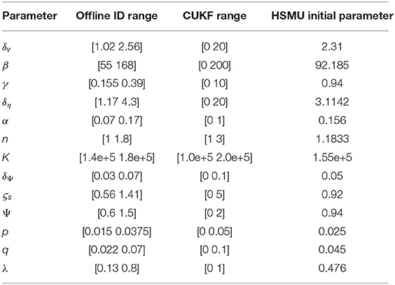
Table 1. Model parameters of Bouc-Wen model.

TABLE 2

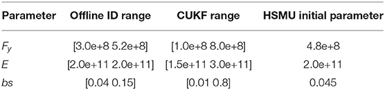
Table 2. Model parameters of bilinear steel material.

In HSMU case I, the numerical model to be updated is the Bouc-Wen model, and the state vector contains 13 parameters and two states. During model updating, noise and estimation tolerance R is determined at 100 N, disturbance matrix Q = diag[10⁻⁶, 10⁻⁴, 10⁻⁴, 10⁻⁵, 10^−4.5,10⁻⁴, 10⁴, 10⁻⁵, 10⁻⁶, 10⁻⁶, 10⁻⁶, 10⁻⁶, 10⁻⁵, 10⁻¹², 10⁻¹²], and an initial variance matrix of P₀ = 10 × I₁₅. These model-updating-related parameters (Q, R, P₀) are still determined on a case-by-case basis. The selection of R and Q and their effect to model updating performance are discussed in Ou et al. (2017).

The online updating results are illustrated in Figure 4. For the first 20 s (S1), the results confirm that most of the Bouc-Wen model parameters can converge 3 s after the testing starts and where the first peak response occurs. A total of 20 s (S2) later, the structural response reaches a larger peak due to the increased ground excitation. Most of the parameters vary and settle to another optimal state. It may be concluded that the parameters have only converged to a local optimum in S1. When the peak response evolves in S2, the converged parameters in S1 can no longer represent the specimen behavior. Therefore, the model updating algorithm continues to adjust the model parameters and brings them to a new converged set.

FIGURE 4

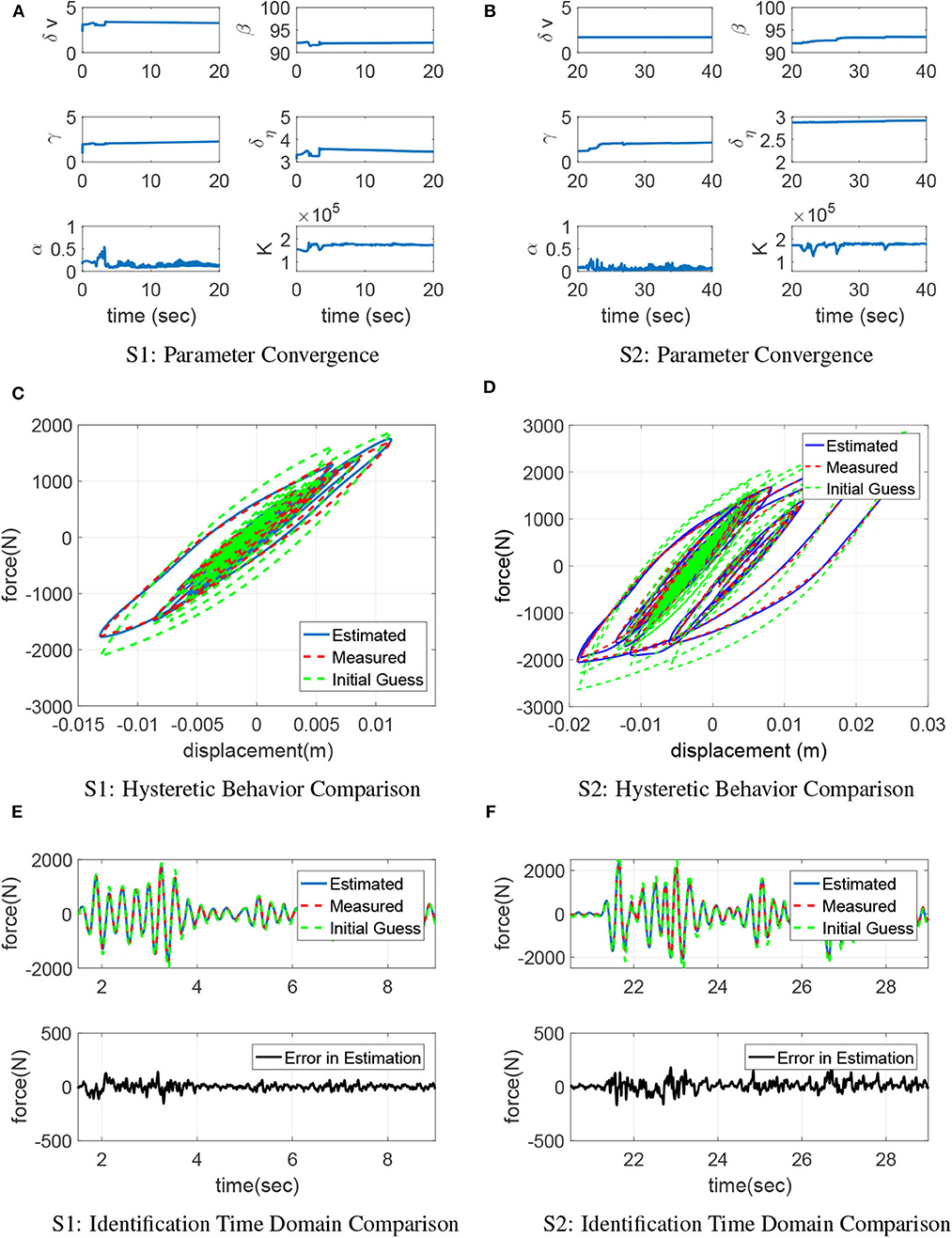
Figure 4. Model updating performance using Bouc-Wen model. (A) S1: parameter convergence, (B) S2: parameter convergence, (C) S1: hysteretic behavior comparison, (D) S2: hysteretic behavior comparison, (E) S1: identification time domain comparison, (F) S2: identification time domain comparison.

Along the entire time history, the Bouc-Wen model can well represent the steel frame nonlinearity. The error between model estimation and measured response is negligible with RMS error of 3.04, 3.59, and 3.34% for S1, S2, and the entire time history, compared to the RMS error in the initial model which is 21.39, 25.32, and 22.78%, respectively. CUKF is effective in updating the phenomenological parameters.

In HSMU case II, only three parameters are identified in the bilinear model. During model updating, noise and estimation tolerance R is also determined to be 100 N, Q = diag[10⁻⁵, 10⁻⁵, 10⁻⁷], P₀ = 10 × I₃, L = 3, and λ_L = −1. Lower-bound d_k and upper-bound e_k of constrained parameters are listed in Table 2. According to the persistence excitation requirement Astrom and Wittenmark (2013), parameters converge faster after the earthquake starts, as in Figures 5A,B. In S1, the estimated yield stress F_y is reduced from the initial parameter 480N/m² to 380N/m², Young's modulus E and the hardening factor b_s did not change. In S2, when a larger peak response occurs, this convergence is clearly affected, and eventually converged to $F_y=560N/m^2$ and b_s = 0.04. Later in S2, the level of nonlinearity evolves where the deformation of structural component increases, the material settles at the second curve where the yield stress is 480N/m² and the reduction factor is around 0.05. The final estimation performs better than the initial guess in S2. From the sequential ground motion, it can be concluded a bilinear curve is not sufficient to describe the steel property since a trilinear behavior is revealed.

FIGURE 5

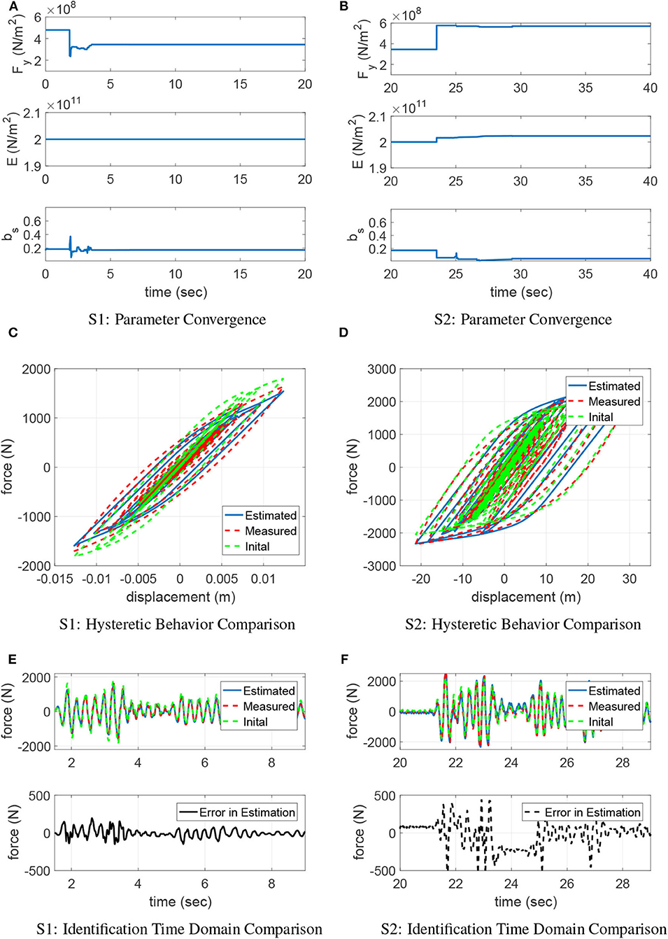
Figure 5. Model updating performance case II. (A) S1: parameter convergence, (B) S2: parameter convergence, (C) S1: hysteretic behavior comparison, (D) S2: hysteretic behavior comparison, (E) S1: identification time domain comparison, (F) S2: identification time domain comparison.

Figure 5C illustrates that initial model underestimates the energy dissipated by the physical component in S1. Later in S2 as shown in Figure 5D, both initial model and updated model have similar behavior. Figures 5E,F show the time history comparison between the measured force R^E, the estimated output R_est, and the difference (error) between the two. In S1, frame hysteresis behavior is improved in HSMU with an RMS error of 8.39% where the initial model yields an RMS error of 26.41%. In S2, the parameters converge at a new optimal, the estimation RMS error in HSMU is 15.11%, which does not improve significantly as the RMS error is 19.85% using the initial guess parameters.

In addition, the results illustrate that the model-updating performance is associated with the choice of the model. Comparing the model-updating accuracy of case I and II, the RMS error for the entire time history is 3.34% for case I and 13.21% for case II because the Bouc-Wen model can better capture the steel frame hysteresis than the bilinear model. The model-updating performance further affects the fidelity of hybrid simulation results. The RMS errors between two model updating cases are summarized in Table 3.

TABLE 3

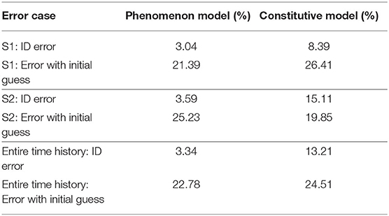
Table 3. RMS error in two model updating cases.

4.2. Global Response Comparison Between HSMU and Shake Table Testing

Displacement and acceleration responses from two HSMUs (labeled as HSMU-BW and HSMU-BL) are compared to the measured responses of an experimental shake table testing. In addition, two numerical simulations are conducted, using the initial values of the phenomenon and constitutive model, respectively.

Besides the RMS error index, two additional indicators are introduced to quantify the peak responses error between each HSMU or simulation result and shake table test result, and several critical response peaks are indicated in Figure 6, labeled from A to I.

$\begin{array}{ll}{J}_{1,j}={\displaystyle \sum _{i=1}^5}\frac{x_j(i)-x_{s,j}(i)}{{\displaystyle {\sum }_{i=1}^5}{x}_{s,j}(i)}& (19)\end{array}$

$\begin{array}{ll}{J}_{2,j}={\displaystyle \sum _{i=1}^5}\frac{{ẍ}_j(i)-{ẍ}_{s,j}(i)}{{\displaystyle {\sum }_{i=1}^5}{ẍ}_{s,j}(i)}& (20)\end{array}$

where J₁ is the peak displacement error, J₂ is the peak acceleration error, x_s indicates measured displacement from shake table test, ẍ_s indicates measured acceleration from shake table test, and j is the profile number (A to I).

FIGURE 6

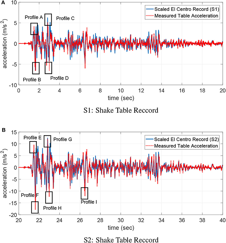
Figure 6. Shake table ground motion records. (A) S1: shake table record, (B) S2: shake table record.

In S1 (0–20 s), the entire structure is excited with the first set of El-Centro ground motion. Figure 7 illustrates the time domain displacement and the acceleration responses from two HSMUs and the shake table test on the top floor. It shows consistent matching between HSMU-BW and the shake table response, with only slightly undershoot after 14 s. This undershoot of HSMU-BW may be introduced by the overestimation of the energy dissipation of the Bouc-Wen model when interstory displacement is small. For HSMU-BL, overshoots in both displacement and acceleration are observed. This observation aligned with conclusions from the local assessment that the bilinear constitutive model cannot well captured the Bauschinger effect of the steel frame, and therefore underestimates the energy dissipation. Later in S2 (20–40 s), the entire steel frame is excited by a larger magnitude El-Centro earthquake with peak ground acceleration reaches 18.3 m²/s. The first story frame experiences a peak drift at 21.5 s, labeled as location E. Later after E, a residual drift is observed as shown in Figure 8 for top floor displacement. However, residual drifts are quite difficult to capture with high accuracy, both HSMU-BW and HSMU-BL cases fail to match measured displacements in shake table exactly. Some possible explanations can be (1) deficiency in the connection manufacturing; (2) a fixed-end simplification of the connection is not sufficient; and (3) the inertia effect is numerically applied. Further studies to improve the residual drift prediction using simulation model are needed.

FIGURE 7

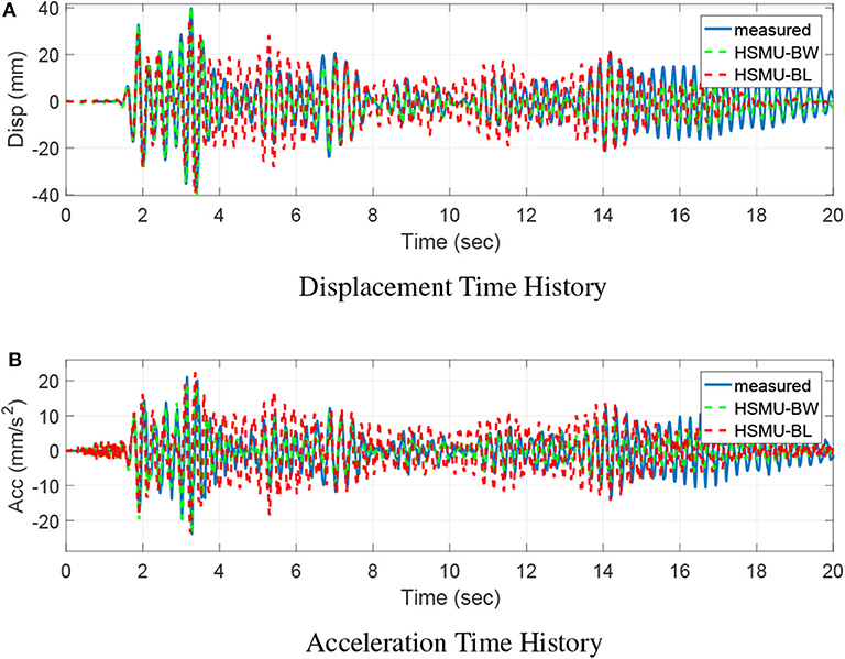
Figure 7. S1: Top floor time history responses. (A) Displacement time history, (B) Acceleration time history.

FIGURE 8

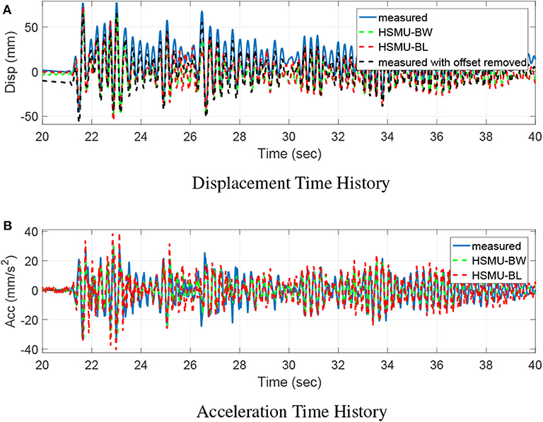
Figure 8. S2: Top floor time history responses. (A) Displacement time history, (B) Acceleration time history.

HSMU and shake table test data are analyzed in the frequency domain as well, and results are shown in Figure 9. Some observations are made: (1) the first and second modes are off for Sim-BW and Sim-BL after updating cases (HSMU-BW and HSMU-BL) have improved their accuracy; (2) the Bouc-Wen model overestimated the damping of the structure, even after the model updating, and, in contrast, the bilinear model always underestimated this damping/energy dissipation; (3) results indicate the model updating is effective for both models. However, the selection of the model can be more dominant after the parameters of the selected model is correctly calibrated.

FIGURE 9

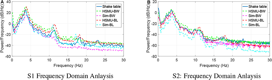
Figure 9. Frequency domain analysis. (A) S1: frequency domain analysis, (B) S2: frequency domain analysis.

Displacement profiles are further compared and demonstrated in Figures 10A,B. A simulation using initial Bouc-Wen model parameters (SIM-BW) underestimates the maximum displacement in profile B, C, and D, which is similar to what was discussed in the frequency analysis. The quantified displacement errors are listed in Table 4. In the first section, HSMU-BW has the least error for profile A, C, and D, and SIM-BW has the largest error for all peaks. The improvement is significant after model updating, and total error reduces from 1.526 to 0.1681. Error in the displacement is only slightly reduced from 0.4492 to 0.4021 as comparing the HSMU-BL with the SIM-BL. One explanation is that the model-updating efficiency is taken over by the inherent modeling error (the selected model is not sufficient to represent a certain behavior) in the bilinear model case. In the second section, J₁ index reaches its maximum at peak location F for all cases, which is the first response peak (in the reverse direction) after the residual drift occurred at E. This can also be visualized in Figure 10B. In displacement profile G-I, due to the existence of the residual drifts on each story, the error indicators do not represent the performance well. Results are more informative in the acceleration responses.

FIGURE 10

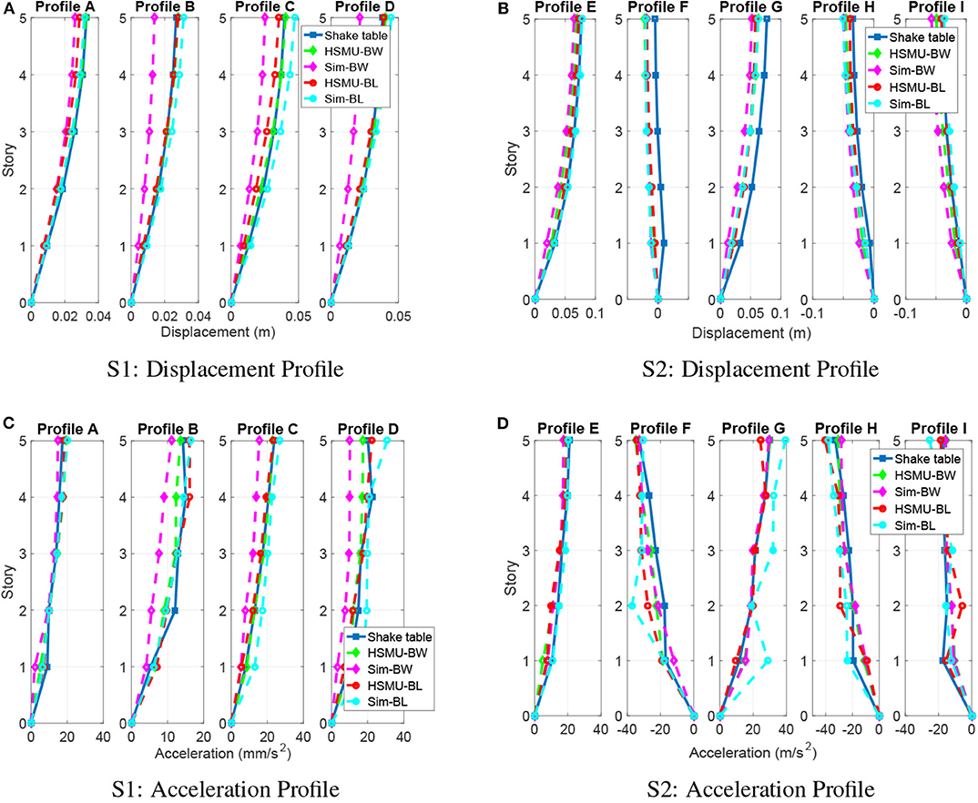
Figure 10. Displacement and acceleration profiles at peak locations. (A) S1: displacement profile, (B) S2: displacement profile, (C) S1: acceleration profile, (D) S2: acceleration profile.

TABLE 4

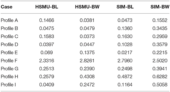
Table 4. J₁ Peak displacement error.

Figures 10C,D illustrates the acceleration profiles, and Table 5 listed J₂ errors, for all cases. In S1, the same observations as in the displacement profiles are observed at peak A to D. In S2, HSMU-BW yields the smallest error in J₂, which indicates the responses are more accurate. This error is reduced from 1.5968 from the SIM-BW, the largest error among all the cases. For the bilinear case, by comparison with S1, the acceleration response improvement is more significant, as J₂ decreases from 1.43, as in SIM-BL, to 0.95, as in HSMU-BL. It may be concluded that (1) the model-updating process is very effective for the phenomenological model and is adaptive to different excitation amplitudes, and (2) the main reason for such improvement in HSMU fidelity is due to the first floor response measured from the experimental substructure. Even the bilinear model cannot capture the Bauschinger effect well for upper stories, and the critical first floor response is the true response from the specimen.

TABLE 5

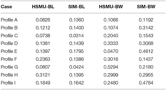
Table 5. J₂ Peak acceleration error.

5. Conclusion

Model updating is introduced into hybrid simulation to improve the fidelity of the testing when components similar to the physical specimen are also present in the numerical substructure. To understand how model updating in hybrid simulation improves the experimental fidelity, this paper compared HSMU results to shake table results. Both the phenomenological Bouc-Wen model and bilinear steel constitutive finite element model were used in the numerical substructure and have been updated. The main conclusions of this study are as follows:

• Overall, the HSMU approach can be successfully implemented to concentrated Bouc-Wen and distributed material nonlinear models. The parameters for each model can converge adaptively under different excitation intensities.

• From the local assessment, the Bouc-Wen model better captured the hysteresis behavior of the experimental substructure, which is also more responsive to model updating. However, the initial parameter selection for Bouc-Wen model is not intuitive. In contrast, the bilinear model cannot well capture the Bauschinger effect of the steel frame, the model error introduced by the model selection overruled the parameter updating improvement. Despite this, the determination of its initial parameters is less arbitrary.

• From the global assessment, frequency domain analysis is carried out for all HSMUs and simulations, and results indicated that significant improvement is observed in both HSMU cases. The first modes of the structure after model updating are much more accurate compared to the first modes resulted from the initial models.

• In the time domain analysis, results indicate the Bouc-Wen model may overestimate the energy dissipation or damping of the components, and the HSMU-BW case shows undershoots of peak responses. In the bilinear finite element model, energy dissipation is always underestimated, which resulted in overshoots at response peaks. This observation matched the local assessment observations as well.

• The steel frame developed large residual drift on the first floor after the peak strike of the larger ground motion (S2). Neither HSMU-BW nor HSMU-BL case can exact estimate this residual drift, which still is a challenging topic for seismic analysis in general.

• The main reason for such improvement in HSMU fidelity is due to the first floor response measured from the experimental substructure. Even the bilinear model cannot capture the Bauschinger effect well for upper stories, and the critical first floor response is the true response from the specimen.

After all, in HSMU, it should be the users to decide the tradeoff between the modeling accuracy based on model selection and its complexity. Other constitutive models such as Menegotto-Pinto model can be a desired alternative. Different model updating algorithms that are robust with larger experimental and numerical uncertainties and that are adaptive to model selection instead of parameter identification should be developed in the later studies.

Data Availability Statement

The datasets generated for this study are available on request to the corresponding author.

Author Contributions

All authors listed have made a substantial, direct and intellectual contribution to the work, and approved it for publication.

Funding

This material was based upon work supported by the National Science Foundation under Grant CNS 1136075 and National Natural Science Foundation of China, Joint Research Grant 91315301-9. The author would like to also acknowledge Purdue University Bilsland Fellowship for the financial support.

Conflict of Interest

The authors declare that the research was conducted in the absence of any commercial or financial relationships that could be construed as a potential conflict of interest.

References

Astrom, K. J., and Wittenmark, B. (2013). Adaptive Control. Courier Corporation.

Google Scholar

Baber, T., and Noori, M. N. (1985). Random vibration of degrading, pinching systems. J. Engrg. Mech. 111, 1010–1026. doi: 10.1061/(ASCE)0733-9399(1985)111:8(1010)

CrossRef Full Text | Google Scholar

Baber, T., and Wen, Y. K. (1981). Random vibration of hysteretic degrading systems. J. Engrg. Mech. 107, 1069–1089.

Google Scholar

Christenson, R., Lin, Y. Z., Emmons, A., and Bass, B. (2008). Large-scale experimental verification of semiactive control through real-time hybrid simulation 1. J. Struct. Eng. 134, 522–534. doi: 10.1061/(ASCE)0733-9445(2008)134:4(522)

CrossRef Full Text | Google Scholar

Elanwar, H. H., and Elnashai, A. S. (2016). Framework for online model updating in earthquake hybrid simulations. J. Earthquake Eng. 20, 80–100. doi: 10.1080/13632469.2015.1051637

CrossRef Full Text | Google Scholar

Elnashai, A. S., Spencer, B. F., Kim, S. J., Holub, C. J., and Kwon, O. S. (2008). Hybrid distributed simulation of a bridge-foundation-soil interacting system,” in The 4th International Conference on Bridge Maintenance, Safety, and Management (Seoul).

Gao, X., Castaneda, N., and Dyke, S. J. (2013). Real time hybrid simulation: from dynamic system, motion control to experimental error. Earthq. Eng. Struct. Dyn. 42, 815–832. doi: 10.1002/eqe.2246

CrossRef Full Text | Google Scholar

Gomez, D., Dyke, S. J., and Maghareh, A. (2014). Enabling role of hybrid simulation across NEES in advancing earthquake engineering. Smart Struct. Syst. 15, 913–929. doi: 10.12989/sss.2015.15.3.913

CrossRef Full Text | Google Scholar

Hakuno, M., Shidawara, M., and Hara, T. (1969). Dynamic destructive test of a cantilever beam, controlled by an analog-computer. Trans. Jpn. Soc. Civil Eng. 171:a1. doi: 10.2208/jscej1969.1969.171_1

CrossRef Full Text | Google Scholar

Hashemi, M. J., Masroor, A., and Mosqueda, G. (2014). Implementation of online model updating in hybrid simulation. Earthq. Eng. Struct. Dyn. 134, 395–412. doi: 10.1002/eqe.2350

CrossRef Full Text | Google Scholar

Kandepu, R., Imsland, L., and Foss, B. A. (2008). “Constrained state estimation using the unscented Kalman filter,” in Proceedings of the 16th Mediterranean Conference on Control and Automation (New York, NY: Institute of Electrical and Electronics Engineers), 1453–1458.

Google Scholar

Karavasilis, T. L., Ricles, J. M., Sause, R., and Chen, C. (2011). Experimental evaluation of the seismic performance of steel MRFs with compressed elastomer dampers using large-scale real-time hybrid simulation. Eng. Struct. 33, 1859–1869. doi: 10.1016/j.engstruct.2011.01.032

CrossRef Full Text | Google Scholar

Kwon, O. S., and Kammula, V. (2013). Model updating method for substructure pseudo-dynamic hybrid simulation. Earthq. Eng. Struct. Dyn. 42, 1971–1984. doi: 10.1002/eqe.2307

CrossRef Full Text | Google Scholar

Lin, P. C., Tsai, K. C., Wang, K. J., Yu, Y. J., Wei, C. Y., Wu, A. C., et al. (2012). Seismic design and hybrid tests of a full-scale three-story buckling-restrained braced frame using welded end connections and thin profile. Earthq. Eng. Struct. Dyn. 41, 1001–1020. doi: 10.1002/eqe.1171

CrossRef Full Text | Google Scholar

Mahin, S. A., and Shing, P. S. (1985). Pseudodynamic method for seismic testing. J. Struct. Eng. 111, 1482–1503. doi: 10.1061/(ASCE)0733-9445(1985)111:7(1482)

CrossRef Full Text | Google Scholar

Ou, G., and Dyke, S. J. (2016). “Real time hybrid simulation with online model updating on highly nonlinear device,” in Rotating Machinery, Hybrid Test Methods, Vibro-Acoustics & Laser Vibrometry, Vol. 8 (Cham: Springer), 343–350.

Google Scholar

Ou, G., Dyke, S. J., and Prakash, A. (2017). Real time hybrid simulation with online model updating: an analysis of accuracy. Mech. Syst. Signal Process. 84, 223–240. doi: 10.1016/j.ymssp.2016.06.015

CrossRef Full Text | Google Scholar

Ou, G., Ozdagli, A. I., Dyke, S. J., and Wu, B. (2015). Robust integrated actuator control: experimental verification and real-time hybrid-simulation implementation. Earthq. Eng. Struct. Dyn. 44, 441–460. doi: 10.1002/eqe.2479

CrossRef Full Text | Google Scholar

Phillips, B. M., and Spencer, B. F. Jr. (2012). Model-based feedforward-feedback actuator control for real-time hybrid simulation. J. Struct. Eng. 139, 1205–1214. doi: 10.1061/(ASCE)ST.1943-541X.0000606

CrossRef Full Text | Google Scholar

Shao, X., Mueller, A., and Mohammed, B. A. (2016). Real-time hybrid simulation with online model updating: methodology and implementation. J. Eng. Mech. 142:04015074. doi: 10.1061/(ASCE)EM.1943-7889.0000987

CrossRef Full Text | Google Scholar

Song, W., and Dyke, S. (2013). Real-time dynamic model updating of a hysteretic structural system. J. Struct. Eng. 140:04013082. doi: 10.1061/(ASCE)ST.1943-541X.0000857

CrossRef Full Text | Google Scholar

Wu, B., and Wang, T. (2015). Model updating with constrained unscented Kalman filter for hybrid testing. Smart Struct. Syst. 14, 1105–1129. doi: 10.12989/sss.2014.14.6.1105

CrossRef Full Text | Google Scholar

Yang, G., Wang, Z., Wu, B., Yang, J., Xu, G., and Chen, Y. (2015). Development of hyTest for structural hybrid simulation. J. Build. Struct. 36, 149–156. doi: 10.14006/j.jzjgxb.2015.11.019

CrossRef Full Text

Yang, G., Wu, B., Ou, G., Wang, Z., and Dyke, S. (2017). HyTest: Platform for structural hybrid simulations with finite element model updating. Adv. Eng. Softw. 112, 200–210. doi: 10.1016/j.advengsoft.2017.05.007

CrossRef Full Text | Google Scholar