Aeroelastic Testing of Span-Wire Traffic Signal Systems

Introduction

Geographically, Florida and the East Coast of the United States have been very vulnerable to extreme wind events such as hurricanes and thunderstorms. Significant structural damage occurs from such high-intensity winds on an annual basis (Holmes, 2015; Simiu and Yeo, 2019). Of general interest in this paper are civil engineering transportation infrastructure, specifically span-wire traffic signal systems. Such traffic systems are of high importance since a lack of functionality greatly affects traffic flow within a city as well as evacuation plans before or during the passing of such severe events with large geographic footprint. By consequence, the enhancement of traffic signals is of utmost importance to the safety of motorists (Sivarao et al., 2010; Zuo and Letchford, 2010; Irwin et al., 2016; Matus, 2018).

In most cases, traffic conditions and vehicular flow direct the use of certain traffic signal configurations over others. According to the State of Florida Department of Transportation (FDOT), as much as 63% of intersections in the state use span-wire traffic signal systems. Typically, such traffic signal systems consist of the signal units supported by aluminum hangers and two wires (a messenger on the bottom and a catenary on the top) holding the hangers in place and spanning between two poles (typically steel or concrete). Despite their wide use in the state of Florida, there is a lack of design guidelines for span-wire systems subjected to high-intensity wind events (Cook et al., 2012; Irwin et al., 2016; Zisis et al., 2016a, 2017; Azzi et al., 2018, 2019; Matus, 2018). Although mast-arms are preferred to span-wire traffic signals, the use of the latter system remains as the only solution when the installation of a mast-arm is not feasible (Matus, 2018). During the 2004–2005 hurricane season, it was observed that these systems were very susceptible to damages under wind-induced forces, which indicated that a better design was required to enhance their survivability and sustainability (State of Florida Department of Transportation (FDOT), 2005; Cook et al., 2012; Zisis et al., 2016a). More recently, damage assessment studies conducted post-impact of hurricanes Irma and Michael in the state of Florida have showed the vulnerability of traffic signals to strong wind-storms (Pinelli et al., 2018; StEER: Structural Extrement Event Reconnaissance Network, 2018). There have been previous studies on traffic signals, which had found that oscillations, caused by wind-induced forces, can cause structural damages (McDonald et al., 1995). These oscillations were identified as an incipient galloping instability that can produce damages to different components of the traffic signals attached to cantilevered structures (Kaczinski et al., 1998). It is important to enhance the knowledge on the response of the span-wire traffic signal systems as damages may impose life-threatening conditions for motorists during and after extreme wind events (Sivarao et al., 2010). Studies have focused on the effect of wind loads on untethered span-wire signal poles and recommended the consideration of load transfer induced by such forces, which can cause significant deflections to end supports (Alampalli, 1997). Cook et al. (2012) conducted 33 tests of different span-wire traffic signal systems identifying inclination issues as well as hardware failure due to wind-induced forces. Due to the typical span lengths, which can vary from 15 to 60 m length (Irwin et al., 2016), a full-scale test of the traffic signals is difficult and this particular research experiment, conducted by Cook et al. (2012), created hurricane-wind forces (non-ABL) which were applied to 1-signal or 2-signal configurations and not to the entire traffic system. Later investigations carried out in an ABL wind tunnel tested the two most typical span-wire traffic signal configurations used and identified that the most susceptible and/or critical configuration was a 3–3–5 configuration, which consists of two 3-section plus one 5-section signals mounted on a short-span test rig. This investigation also showed that some span-wire traffic signals can undergo aerodynamic instabilities at wind speeds as low as 32 m/s (Irwin et al., 2016; Zisis et al., 2016b). The special short-span rig was designed to produce the same response of a typical 24 m long span-wire traffic signal system by the addition of coil springs at either side of the system cables (Irwin et al., 2016). Other investigations examined the overall response of span-wire traffic signals with different parameters of the signal assembly itself and found out that such changes affect the drag and lift coefficients of the entire system (Matus, 2018). The majority of the previous research has focused on certain components of span-wire traffic signal assemblies due to the difficulty of testing a full-scale span. Zisis et al. (2017) provided valuable validation on the efficacy of a short-span test rig of 6.7 m to represent a 24 m span. It must be noted that as the scale of the model is increased, the ability of the wind tunnel to recreate the full frequency range of the wind turbulence reduces and the aerodynamic buffeting effects may be compromised, failing to provide a full response of the system as well as limiting the length of the span that can be simulated. With the 1:10 aeroelastic model, the full aerodynamic response would be obtained and a study on the effect of different span lengths could be accomplished.

The methodology of this study involves the design and testing of an aeroelastic model of a span-wire traffic system consisting of two 3-section and one 5-section signals subjected to varying wind speeds from various directions. The model is a scaled-down version of an actual span-wire traffic signal assembly previously tested at the NHERI Wall of Wind Experimental Facility (WOW EF) (Irwin et al., 2016; Zisis et al., 2017). Observations pertaining to aerodynamic instabilities were made and the results were compared to those achieved from the earlier full-scale testing. Wind testing of a reduced aeroelastic model representing this particular span-wire configuration allowed a better representation of the wind turbulence spectrum. Such tests also enabled the evaluation of the wind-induced buffeting response of the structure.

Methodology

The Wall of Wind Experimental Facility

The National Science Foundation (NSF) designated FIU's Wall of Wind (WOW) as one of the Experimental Facilities (EFs) under the distributed, multi-user, national Natural Hazards Engineering Research Infrastructure (NHERI). The WOW EF is an open jet testing facility consisting of a 12-fan system. The facility can generate Atmospheric Boundary Layer (ABL) wind speeds and turbulence characteristics, similar to those observed and recorded in hurricanes (up to the intensity of Category 5 in the Saffir-Simpson scale). The test section, which is 6 m wide and 4.3 m high, permits testing of buildings and lifeline infrastructure systems at large scales, as well as full-scale testing of building components, equipment, and rooftop installations, among others. Wind speeds at the WOW are able to reach a maximum of 70 m/s while wind profiles and terrain conditions are simulated by a set of automated roughness elements and spires located in the flow conditioning section. More information about the WOW EF, its capabilities, and enabled research, is available in Chowdhury et al. (2017). Figures 1A,B show the intake side and the flow conditioning section at the WOW.

FIGURE 1

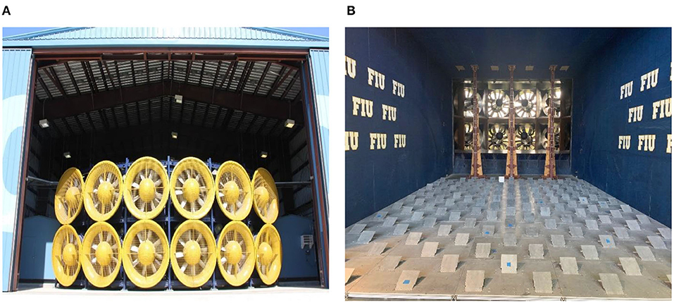
Figure 1. WOW facility: (A) intake side, (B) spires and automated roughness elements [Reproduced from Azzi et al. (2020) under the Creative Commons CC BY license].

Prototype Description

The prototype span-wire traffic signal system chosen for this experiment is a typical assembly that can be found on any two- or more lane roadway, particularly in the state of Florida. Figure 2 illustrates a span-wire traffic signal assembly used in Florida. For the full-scale tests conducted at the WOW, the span-wire traffic signal assembly was composed of the following: (i) two HSS (ASTM Standard A00/A500M, 2018) Grade B steel columns standing at the end-spans having a height of 8.5 m; (ii) two seven-wire strands steel cables (messenger and catenary cables) having a diameter of 9.5 mm and satisfying the properties specified in (ASTM Standard A475, 2014) for Class A Zinc Coating; (iii) three rigid aluminum alloy hangers holding both cables together, and (iv) three traffic signals hanging from the bottom end of the hangers. The messenger cable is tensioned with a uniform axial force of 240 N and the catenary wire is fixed in a way to provide a 5% sag at mid-span. The traffic signals selected for this study consisted of one 5-section and two 3-section signals. Previous research on span-wire traffic systems by Zisis et al. (2016a,b) has shown the above-described configuration as the most vulnerable, and therefore, was used for this investigation.

FIGURE 2

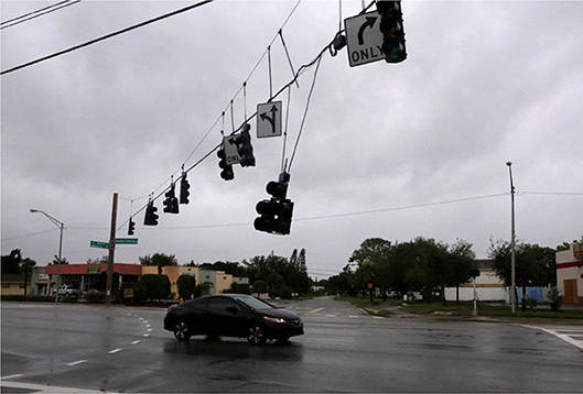
Figure 2. Typical span-wire traffic signal system.

Typically, a span-wire traffic signal system spans between 15 and 60 m, depending on the physical properties of the intersections such as the number of lanes and their width (Irwin et al., 2016). For the full-scale specimen, two spans were considered: a short- and long-span. First, a short-span rig of ~6.7 m was designed and implemented at the WOW. The idea behind the design of the short-span was to be able to fully mount the system on the turntable, thus allowing for multiple wind directions to be tested. Since a span of 6.7 m is not realistic and does not belong to the range mentioned above (between 15 and 60 m), coil-springs were added on both ends of the cables in order to have the same lateral force to deflection properties as the long-span frame (Irwin et al., 2016; Zisis et al., 2017). Both short- and long-span specimens are presented in Figures 3A,B, respectively. More information on the validation between both specimens is available in Zisis et al. (2017).

FIGURE 3

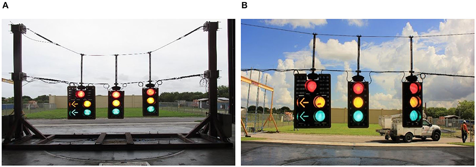
Figure 3. Full-scale specimens: (A) short-span, (B) long-span.

Although full-scale testing provides valuable information on the performance and response of traffic signal components (for instance the focus of the full-scale tests was the detailed evaluation of different hanger connections) mounted on span-wire systems with realistic consideration of structural boundary conditions and system dynamic properties, various limitations are also encountered. Because the tests are conducted at full-scale, and wind tunnels have a limited test section size, it is not feasible to simulate the complete spectrum of wind turbulence as in the real ABL flow (Choi and Kwon, 1998; Mooneghi et al., 2016; Moravej, 2018). Also, in full-scale testing, the exact clearance between the bottom of the traffic signals and the ground, which typically ranges between 4.6 and 6 m, cannot be maintained inside the testing section. On the other hand, scaled aeroelastic testing enables a better simulation of the turbulence spectrum at the natural frequency of the signals. However, at smaller scales, the accuracy of the geometric and mechanical simulation of the components that form the model become quite challenging. Due to the lack of guidelines for the safe design of span-wire traffic signals and because of their wide use, especially in the state of Florida, it is crucial to investigate the dynamic performance of such systems under extreme wind conditions. To the best of the authors' knowledge, no prior studies have been done considering the proper simulation of the dynamic characteristics of the entire system to assess the wind-induced dynamic and aeroelastic response of traffic infrastructure. Such a knowledge gap hinders achieving resilient communities and adverse recovery strategies post hurricane events. Therefore, the main objective of the current study is to perform comparisons between the two wind testing methods (full-scale testing vs. aeroelastic testing) and investigate the adequacy of each individual approach in estimating the overall dynamic response in light of the capacity and limitation of each test. Consequently, it was decided to construct an aeroelastic model with a 1:10 scale of the exact specimen that was tested at full-scale earlier to better investigate the overall dynamic response of the traffic signals and compare its behavior.

Model Description

Laws of Similitude

For this set of experiments, which utilizes a relatively large length scale of 1:10, Froude number similitude was preserved. By definition, a Froude number characterizes the ratio of fluid inertial forces to gravitational and elastic forces of the structure itself. For this particular structural aeroelastic modeling, since the gravitational forces (e.g., the wire vibrations) are more dominant than their frictional counterparts and because of the expected significant movement of the traffic signals (as found in the earlier full-scale study), the selection of Froude number Fr similarity was adopted. Furthermore, since the gravitational acceleration g is kept the same for both prototype and model, then the scaling would be achieved by linking the velocity scale to the square root of the length scale. Note that it is not feasible to satisfy both Fr and Re scaling simultaneously and because of the scaled model approach, the “full-scale Re” simulation was not possible. Lastly, the bluff shapes of the traffic signals are expected to make them less dependent on Re. Hence, there is a need to carefully simulate the distribution of masses and elastic stiffnesses along both prototype and model in order to maintain dynamic similarity and structural response. For any general quantity measured on the prototype Q_P, Equation (1) can be used to calculate its model counterpart Q_M:

$\begin{array}{ll}{Q}_M=Q_P\times {\lambda }_Q& (1)\end{array}$

where λ_Q is the physical property scaling factor.

The relationship between the prototype and the model quantities strongly depend on the materials selected for the construction of the latter. To maintain the structural damping of the system components, prototype materials were selected for the construction of the aeroelastic model. However, due to some constraints regarding the satisfaction of other scaling ratios such as the mass and the stiffness, some elements required a change of material type. Table 1 summarizes the most important scaling factors required for the design of the aeroelastic model.

TABLE 1

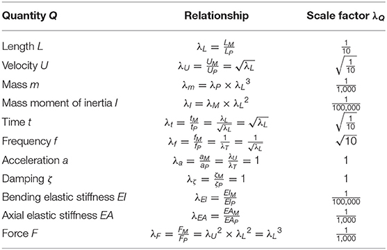
Table 1. Scaling factors λ_Q.

Aeroelastic Design of Cables

The dynamic behavior of any cable structure is dominated by three main properties: its distributed weight per unit length, its diameter, and most importantly, its axial elastic stiffness EA. Note that E is the modulus of elasticity and A is the cross section. The prototype axial elastic stiffness EA was scaled down using the appropriate factor from Table 1 and a diameter of 0.25 mm was selected. Equation (2) states the drag coefficient requirements that need to be satisfied for aeroelastic modeling:

$\begin{array}{ll}{C_D}_M\times D_M={C_D}_P\times D_P\times {\lambda }_L& (2)\end{array}$

where C_DM, C_DP, D_M, and D_P are the drag coefficients of the model and the prototype cables and their diameters, respectively, and λ_L is the length scale factor. Although the previously chosen diameter of 0.25 mm satisfies the axial stiffness scaling requirements, yet, it partially fulfills the drag and weight requirements. This explains the need to add non-structural elements in the form of foam rods along the span of the wires in order to fulfill that purpose. The rods were 9.5 mm thick and 2.3 cm long. By carefully meeting all three requirements related to axial stiffness, diameter, and distributed weight, the frequency and mode shapes of the prototype span-wire system are reproduced at the reduced scale. More details about the design validation are discussed later on in the paper. The actual shape and location of the foam elements can be seen in Figure 4.

FIGURE 4

Figure 4. Aeroelastic model on the WOW turntable.

Aeroelastic Design of Column, Hangers, and Traffic Signals

The column rigs used for the supports of the aeroelastic span-wire traffic signal model were made of aluminum having a solid rectangular cross-section of 2.54 by 1.9 cm. The column section was chosen so that the columns are sufficiently rigid. As for the hangers, thin aluminum sheets with cross-sectional dimensions of 3 by 0.5 mm are selected. Both structural elements are designed according to their bending elastic stiffness EI and their weight W.

For the traffic signals, three units were used: two 3-section and one 5-section. The full-scale signals were weighed and measured at the WOW and then scaled down according to the appropriate factors from Table 1. Consequently, the units were carefully drawn on a CAD software using the scaled-down measurements and considering all the important geometry details (e.g., openings, chamfering of edges, etc.). Moreover, an in-house 3D printer was used to reproduce the small-scale traffic signals using a resin. Since the 3D printed elements are lighter than their aluminum counterparts, their masses were adjusted by installing steel sheets on the inner walls of the signals. This procedure made the signals heavier in order to reach the target mass. Figure 4 shows the small-scale aeroelastic model mounted on the WOW turntable.

Numerical Modeling and Validation

Modal analyses were performed for both full- and small-scale specimens using the Finite Element Methods (FEM) commercial software SAP2000^® (CSI, 2018). All the previously described sectional properties and dimensions (full- and small-scale) were used to reproduce the prototype and the model. The subsequent mode shapes along with their respective frequencies were identified and summarized in Table 2.

TABLE 2

Table 2. Modal analyses results.

The columns were modeled as straight rigid frame elements with fixed supports at the ground level. The hangers were also modeled as rigid frame elements and were clamped to both cables at the desired locations. The wires were represented using cable elements and the traffic signals were drawn as solid sections and their shapes were accurately simulated.

Table 2 shows the two most dominant mode shapes in the behavior of both models. Note that the target frequency is equal to the prototype frequency times the appropriate scaling factor (${\lambda }_f=\sqrt{10}$, Table 1). As can be seen, the target and model frequencies are very close with a maximum percentage difference of about 5.8%. This indicates that the materials and sections chosen for generating the FEM aeroelastic model were appropriate, which gave confidence to proceed with the construction of the model at the WOW.

Moreover, the prototype frequency f_p obtained for mode 1 (0.37 Hz) is very close to the experimentally obtained one using a free vibration test for the full-scale specimen. Figure 5 shows the power spectral density (PSD) of the acceleration of the traffic signals in the short-span full-scale prototype, in the direction normal to the span. The PSD plot was obtained from the response of the accelerometers during wind testing. The percentage difference obtained between the theoretical (0.37 Hz) and experimental values (0.39 Hz) for the prototype is ~5.4%. This indicates once again that the modeling of the prototype was conducted properly, and it was representative of the actual specimen tested at the WOW.

FIGURE 5

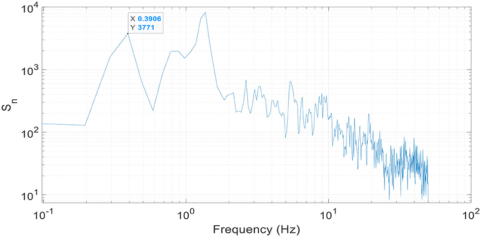
Figure 5. PSD of acceleration for short-span prototype in the direction normal to the span.

Instrumentation and Testing Protocol

The aeroelastic model was instrumented with three 3-axis accelerometers. One accelerometer was installed on the lower backend of each traffic signal. Additionally, and to record the time histories of the velocities, two Cobra probes (Cheung et al., 2003; Cochrane, 2004; McAuliffe and Larose, 2012) were mounted on a rig behind the model at a height of 0.61 m. Data were sampled at a rate of 2,500 Hz for the Cobra probes. Two load cells were installed at the bottom end of each column support. This enabled the recording of the change in tension experienced by the messenger cable.

Open terrain exposure was adopted for this set of tests and the aeroelastic model was exposed to the following wind speeds: 6.5, 9, 11, and 13.5 m/s (corresponding to a full-scale speeds of 21, 28, 35, and 43 m/s at a reference height of 3.2 m). The previous velocities yielded Reynolds number Re values of 1.76 × 10⁵, 2.43 × 10⁵, 2.97 × 10⁵, and 3.65 × 10⁵, respectively. Note that Re values were calculated at a mean signal height of 0.4 m. Also note that, in the full-scale tests, the Re values ranged between 2.2 × 10⁶ and 3.7 × 10⁶ for the different tested wind speeds. Using the automated WOW turntable, several wind directions were investigated, ranging between 0° and 180° at increments of 15°. Note that a wind direction of 0° represents wind approaching normal to the frontend of the traffic signals. Accelerometer and load cell data were sampled at 100 Hz and for a duration of 1 min per exposure angle.

Surface Roughness

Both full-scale and small-scale specimens were tested with the same spires and automated roughness elements that are installed in the flow control box downwind of the fans at the WOW (Figure 1B). Due to the large difference in specimen heights, the surface roughness z_o at the mean height of the traffic signals might have been rougher for the aeroelastic model. Figure 6 portrays the normalized PSD of longitudinal turbulence fluctuations for the aeroelastic model.

FIGURE 6

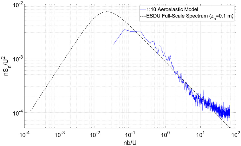
Figure 6. PSD of longitudinal turbulence fluctuations.

Because of the high speeds at which the full-scale tests were run, and so as not to damage the instruments, no cobra probes were used. However, based on previous full-scale tests at the WOW having a similar roughness and spire configuration in the flow chamber, the surface roughness z_o ranged between 0.02 and 0.06 m (Moravej, 2018; Moravej et al., 2019). On the other hand, and according to ESDU (2001), the surface roughness of the aeroelastic tests were about 0.1 m (full-scale). This difference in surface roughness between both specimens might lead to slight divergences in peaks, which could affect the dynamic response comparisons that will follow. Note that in the aeroelastic tests, the turbulence intensity I_u ranged between 10.2 and 12.4% and the integral length scale ^xL_u varied between 0.43 and 0.48 m.

Results and Discussion

In the following section, free vibration test results are reported prior to the actual wind testing findings. Then, the aerodynamic instabilities observed during the entirety of the tests are noted down. In addition, the surface roughness of both full-scale and small-scale specimens are calculated and compared. Furthermore, root-mean-square (RMS) of accelerations are presented and compared to their full-scale counterparts. Last but not least, dynamic amplification factors are calculated for both models. Such a factor allows the investigation of the dynamic response of the system. Furthermore, a buffeting analysis is conducted and theoretical values of RMS of accelerations are calculated and compared with their experimental counterparts.

Free Vibration Tests

A free vibration test prior to the actual start of wind testing was conducted. The purpose of such a test is to compare the recorded natural frequency of the constructed model in the wind tunnel with design values. The test consisted of using a straight wooden rod to manually push back all three traffic signals and let them oscillate freely until reaching their initial rest position while measuring their instantaneous accelerations. This practice allows the recreation of mode shape 1, described in Table 2.

From the captured acceleration time histories, the fluctuating response and the corresponding frequencies can be obtained using a Fast Fourier Transform (FFT) application. Figure 7 depicts the PSD of the acceleration time history of the 5-section traffic signal. Note that the PSD plot has been adjusted to show the full-scale frequency, i.e., the frequency was divided by its respective scaling factor λ_f from Table 1.

FIGURE 7

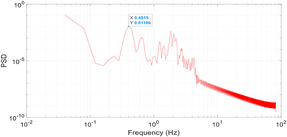
Figure 7. PSD of acceleration of 5-section signal during a free vibration test.

From Figure 7, the frequency of the first mode of vibration, which is defined by the first spike in the curve, occurs around 0.4 Hz (seen in the data box, Figure 7). By comparing the obtained value to the target frequency for mode shape 1 given in Table 2 (0.37 Hz), it can be concluded that the tension in the messenger is nearly equal to the target one and that the model was correctly designed and constructed to mimic the behavior of its full-scale counterpart. Since the reproduction of mode shape 2 (Table 2) was challenging as the traffic signals were rotating around their vertical supports in different patterns, it was decided that matching mode shape 1 was sufficient for the model construction validation.

Observed Instabilities

The aeroelastic model was subjected to wind speeds ranging between 21 and 43 m/s (full-scale) and at angles ranging between 0° and 180° at 15° increments. During the entirety of the test time, some aerodynamic instabilities and natural modes of vibrations were observed, especially from oncoming cornering winds. Figures 8A,B show the aerodynamic instabilities that were most visible during the tests. These instabilities included the appearance of mode shape 1 and some twisting of the 5-section signal around its vertical axis.

FIGURE 8

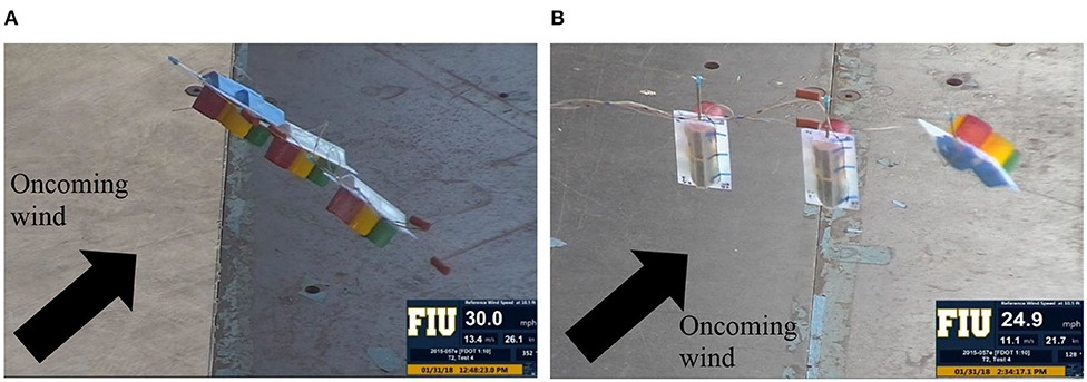
Figure 8. Observed instabilities: (A) backward tilting of all three signals at 0° angle of attack, (B) twisting of 5-section signal at 135° angle of attack.

Figure 8A shows that, at 0° angle of attack and 13.4 m/s, all three traffic signals rotated and tilted backward due to the oncoming wind, illustrating the first natural mode of vibration of the specimen (Table 2). At 135° angle of attack and 11.2 m/s (Figure 8B), and at 45° and 13.4 m/s, more aerodynamic instabilities were observed. Such instabilities included the twisting of the 5-section signal about its vertical axis among others. In other brief instances, the WOW team noticed the appearance of mode shape 2 during the wind testing.

RMS of Accelerations

This section discusses the RMS of the accelerations experienced by the aeroelastic model. As previously mentioned in section Instrumentation and Testing Protocol, three accelerometers were installed on the model, one on the bottom of each of the backplates of the traffic signals. Figure 9A portrays the change in root-mean-square (RMS) of the accelerations experienced by the signals with respect to the increase in oncoming wind speeds at 0° angle of attack, for both models. Note that “A” stands for the RMS of the 5-section signal whereas “B” and “C” belong to each of the 3-section signals. Also, note that the wind speed used is the one at the mean signal height for both specimens and represents the full-scale parameter. In addition, “FS” stands for full-scale and “SS” represents small-scale. More results on the full-scale study for both long-span and short-span specimens is available in Irwin et al. (2016) and Zisis et al. (2017).

FIGURE 9

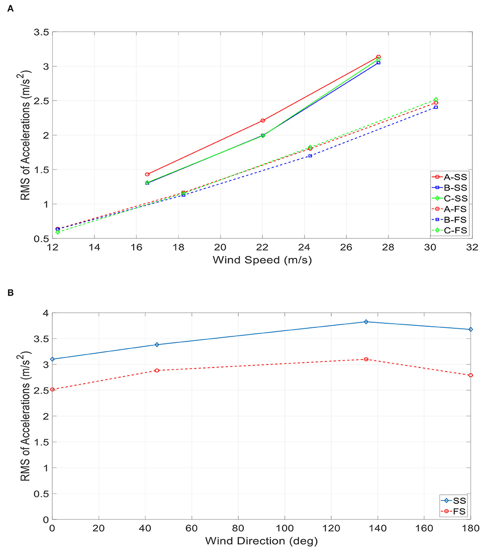
Figure 9. RMS of accelerations at: (A) 0° wind direction, and (B) a wind speed of 27 m/s and different wind directions.

As it can be observed, the results obtained for the aeroelastic model are higher than the full-scale ones for the same approaching speed at the mean height of the traffic signals. The RMS values of the aeroelastic model are around 30–40% higher than the ones experienced by the prototype. However, all values show an approximately linear increasing proportionality relationship between RMS of accelerations and oncoming wind speeds. The same observation was also seen at different wind directions at a wind speed of 27 m/s (this is corresponding to the “full-scale” wind speed at the center of the traffic signals for the full-scale short-span rig and the aeroelastic model) (Figure 9B).

The higher values obtained for the aeroelastic model could be attributed to the better representation of the turbulence spectrum that could be achieved at the small-scale (Figure 6). In addition, the power spectrum value of the response at the model natural frequency in the aeroelastic model was much higher than in the full-scale tests, and at a level that gave a good indication of the resonant response caused by turbulence buffeting from the approaching turbulence. However, in the full-scale tests, the effects of signature turbulence from the signals themselves tended to dominate the entirety of the testing.

Dynamic Amplification Factors

One step in assessing the buffeting response of the traffic signals is to try and decompose the dynamic response of the system into peak, mean, background and resonance. This section introduces the concept of a dynamic amplification factor (DAF). According to Elawady et al. (2017), the DAF is defined as the ratio of the maximum peak response over the maximum quasi-static response, as shown in Equation (3):

$\begin{array}{ll}\text{DAF}=\frac{Maximumpeakresponse}{Maximumquasi-staticresponse}& (3)\end{array}$

where the maximum quasi-static response is the summation of the mean and absolute maximum of the background responses. Note that the resonant response is associated with resonant amplification due to components (accelerations, forces, moments, etc.) with frequencies close or equal to the fundamental natural frequency of the structure. On the other hand, the background response involves no resonant amplification (Simiu and Yeo, 2019).

In brief, the concept of the DAF revolves around to the need to distinguish between the resonant and background components of response fluctuations. The procedure adopted in this study requires calculating and plotting the PSD of the fluctuating response (without the mean) and the corresponding frequencies with the application of a Fast Fourier Transform (FFT). Then, the cumulative PSD of the fluctuating response at each identified frequency is calculated and then normalized to the variance of the fluctuating response PSD. Using the PSD and cumulative PSD of the fluctuating response, the average slope of the common logarithmic values of two successive data points in the PSD of the fluctuating response is divided by the same variable pertaining to two successive data points in the cumulative PSD. At resonance, it is expected that this ratio will be noticeably high, and thus, the detected frequency is marked as resonance frequency. Consequently, once all the resonance frequencies have been identified, a Bandstop filter is adopted to separate the resonance frequencies from the fluctuating responses. The result of that process is the background response. For more details on the procedure, it is advised to refer to Elawady et al. (2017).

Once more, it is expected that the 1:10 aeroelastic model will experience a higher dynamic response compared to its full-scale counterpart due to a better representation of the turbulence spectrum, especially at the low-frequency range (large eddies). The role of analyzing the DAF of the accelerations experienced by both specimens is to separate the resonance from the fluctuating response. The calculation of the DAF of the acceleration will help in better estimating the response of the traffic signals to dynamic loading. Consequently, this will give a better insight into the design of span-wire traffic signals. Figure 10 shows one sample of the processed PSD plot obtained when decomposing the resonance of the acceleration of one traffic signal (Signal “A”) at one wind speed (16.5 m/s at mean signal height) and for one wind direction (0°). The process adopted for this study followed the dynamic response decomposition recommendations described by Elawady et al. (2017). Consequently, the maximum DAF values for accelerations at different wind speeds and for different angles of attacks are calculated and presented in Table 3, for both full- and small-scale specimens. Note that only two accelerometers were installed in the full-scale tests, one on signal “A” and one on signal “C,” hence, there are no available values for DAF of signal “B.”

FIGURE 10

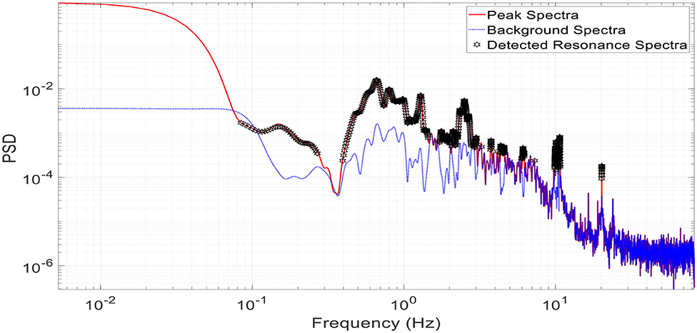
Figure 10. Decomposition of resonance for the acceleration time history of signal “A” (16.5 m/s at 0° wind direction).

TABLE 3

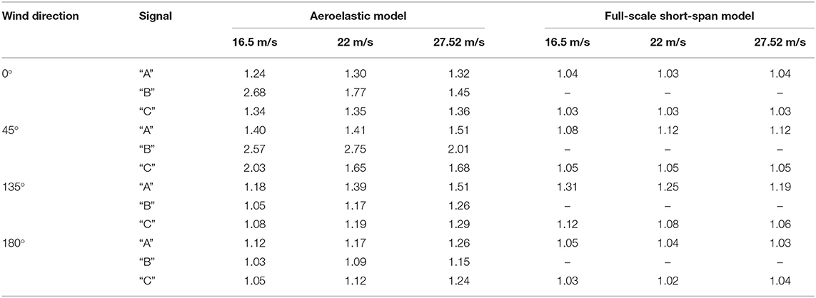
Table 3. DAF results for both specimens in the along-wind direction (wind speeds are converted to full-scale).

By observing Table 3, it can be noted that the DAF values calculated from the aeroelastic model data are generally higher than the ones obtained from the full-scale prototype by around 20–30%. As previously mentioned, a higher dynamic response exhibited by the aeroelastic model can be justified by the presence of more low-frequency turbulence, i.e., a better representation of the low-frequency part of the turbulence spectrum. Recommendations regarding the design of span-wire traffic signals could be formulated using the obtained DAF values. Static design values of accelerations could be multiplied by a uniform DAF value in order to account for dynamic effects.

Buffeting Analysis for RMS of Accelerations

This last subsection discusses the theoretical buffeting of a flexible line-like structure such as the case of span-wire traffic signal systems. By conducting a buffeting analysis on the response of the traffic signals in the longitudinal direction, one can determine the theoretical variance and RMS of acceleration fluctuations and compare the values with experimentally obtained ones. To perform the buffeting analysis, some assumptions need to be made:

• While the instantaneous turbulence velocities at different points are different, the turbulence is homogeneous along the span.

• Using a quasi-steady approach, the fluctuating wind loads can be determined from the aerodynamic force coefficients measured in a steady flow.

• The motions involved in the natural modes of vibration are purely in the along-wind direction or 0° (wind normal to front-end of traffic signals).

• All three traffic signals are treated as one single unit. The single unit has a mass and frontal area equal to the combined masses and frontal areas of all three traffic signals.

Consequently, in its simplified form, the power spectrum of deflection S_q at the mean height of the signals is given by Equation (4) (Davenport, 1962a,b; Irwin, 1977, 1979, 1996):

$\begin{array}{r}{S}_q(n)=\frac{{(\rho .U.C_{x0}.A)}^2}{M_G^2{\omega }_0^4}.|H\left(\frac{n}{n_0},{\zeta }_{tot}\right){|}^2.|{\chi }_y(n){|}^2.|{\chi }_{2D}(n){|}^2\\ \begin{array}{l}.S_u(n)\end{array}& (4)\end{array}$

where ρ is the density of air in kg/m³, U is the wind speed at mean signal height in m/s, C_xo is the drag coefficient of the traffic signal, A is the frontal area of the traffic signal in m², M_G is the mass of the signal in kg and ω_o is the natural angular frequency of the system in rad/s. In addition, n and n_o are the forcing and natural frequencies in Hz, ζ_tot is the total damping of the structure (mechanical + aerodynamic), H(n/n_o, ζ_tot) is the mechanical admittance function, χ_y(n) and χ_2D(n) are the lateral aerodynamic admittance function and two-dimensional admittance function, respectively. Furthermore, S_u(n) is the power spectrum of the longitudinal wind speed time history. To obtain the variance of the deflection fluctuations ${\sigma }_q^2$ from the power spectrum, Equation (4) is integrated over all frequencies and the RMS of the deflection σ_q can then be expressed in terms of background and resonant terms using Equation (5):

$\begin{array}{ll}{\sigma }_q=\frac{\rho .U^2.C_{x0}.A.I_u}{M_G.{\omega }_0^2}.\sqrt{B+R}& (5)\end{array}$

where I_u is the turbulence intensity and B and R are the background and resonant terms, defined in Equations (6) and (7), respectively:

$\begin{array}{ll}B={\displaystyle {\int }_0^{\infty }}|{\chi }_y(n){|}^2.|{\chi }_{2D}(n){|}^2.\frac{S_u(n)}{{\sigma }_u^2}dn& (6)\end{array}$

$\begin{array}{ll}R=|{\chi }_y(n){|}^2.|{\chi }_{2D}(n){|}^2.\frac{n_0.S_u(n_0)}{{\sigma }_u^2}.\frac{\pi }{4.{\zeta }_{tot}}& (7)\end{array}$

where ${\sigma }_u^2$ is the variance of the wind speed time history. The rest of the parameters of Equation (7) are defined in Equations (8–10):

$\begin{array}{l}|{\chi }_y(n){|}^2.|{\chi }_{2D}(n){|}^2=\frac{4}{{\eta }_b^2.{\eta }_d^2}.\left({\eta }_b-1+e^{{-\eta }_b}\right).\left({\eta }_d-1+e^{{-\eta }_d}\right).\\ \begin{array}{l}\frac{2}{{\eta }_L^2}.({\eta }_L-1+e^{{-\eta }_l})\end{array}& (8)\end{array}$

$\begin{array}{ll}\frac{n_0.S_u(n_0)}{{\sigma }_u^2}=\frac{4.\frac{n_0{.}^x{L}_u}{U}}{{(1+70.78.{(\frac{n_0{.}^x{L}_u}{U})}^2)}^{5/6}}& (9)\end{array}$

$\begin{array}{ll}{\zeta }_{tot}={\zeta }_s+{\zeta }_a={\zeta }_s+\frac{\rho .U.C_{x0}.d}{2.{\omega }_0.M_G}& (10)\end{array}$

In the previous equations, η_b, η_d, and η_L are parameters linked to the width, depth, and length of the structure and defined in Equations (11–13). ^xL_u is the integral length scale of longitudinal component of turbulence in the x-direction (normal to the traffic signal) in m, ζ_s is the damping ratio of the structure, ζ_a is the aerodynamic damping and d is the depth of the traffic signal. In Equations (12) and (13), ^yL_u and ^zL_u are the integral length scales of the longitudinal component of turbulence in the y- (lateral) and z-direction (vertical), respectively, in m. Moreover, θ is taken as 0.75 and b along with L are the width and length of the traffic signal in m:

$\begin{array}{ll}{\eta }_b=\mathrm{0.95.}\theta .\frac{b}{{{}^{x}L}_u}.{(1+\mathrm{70.78.}{(\frac{n.{{}^{x}L}_u}{U})}^2)}^{1/2}& (11)\end{array}$

$\begin{array}{ll}{\eta }_d=\mathrm{0.475.}\theta \frac{d}{{{}^{z}L}_u}.{(1+\mathrm{70.78.}{(\frac{2.n.{{}^{z}L}_u}{U})}^2)}^{1/2}& (12)\end{array}$

$\begin{array}{ll}{\eta }_L=\mathrm{0.475.}\theta .\frac{L}{{{}^{y}L}_u}.{(1+\mathrm{70.78.}{(\frac{2.n.{{}^{y}L}_u}{U})}^2)}^{1/2}& (13)\end{array}$

Subsequently, the acceleration spectrum may be obtained by multiplying the deflection spectrum (Equation 5) by circular frequency to power 4. Typically, the resonant portion of the spectrum is the dominant one and the background response can be taken as zero. Therefore, the RMS of the acceleration σ_a reduces to the relatively straightforward expression, given in Equation (14):

$\begin{array}{ll}{\sigma }_a=\frac{\rho .U^2.C_{x0}.A.I_u}{M_G}.\sqrt{R}& (14)\end{array}$

By using Equation (14), the RMS of acceleration values at different wind speeds for both full- and small-scale specimens can be calculated and compared with their experimental counterparts, presented in Figure 9A at 0° wind direction. In order to apply some of the previous equations, more assumptions must be made. First, the three traffic signals are treated as a single unit having the following full-scale dimensions: a frontal area of about 2.6 m² and a mass of 103 kgs. Concerning turbulence correlation effects, it is assumed that they happen for a total length of 3.66 m, a total height of 1.52 m and a total width of 0.33 m (full-scale). The remaining values obtained for all the parameters listed in Equations (7–14) for the aeroelastic model for a wind speed of 27 m/s are summarized in Table 4.

TABLE 4

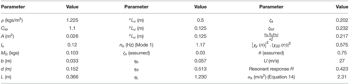
Table 4. Buffeting analysis conducted on the aeroelastic model for a wind speed of 27 m/s and at a wind direction of 0°.

From Table 4, the obtained RMS of acceleration σ_{a, th} value using the theoretical buffeting analysis approach yielded a value of about 2.31 m/s². By inspecting Figure 9A, σ_{a, ex} obtained from the recorded time histories of the accelerometers for the aeroelastic model is about 3 m/s² at a wind speed of 27 m/s. The obtained value from the buffeting analysis is lower than that observed in Figure 9A. However, it is worthwhile noting that the buffeting analysis does not take into account any excitation of the model due to self-generated wake turbulence. If we assume such excitation to be around 1.8 m/s² for both aeroelastic and full-scale specimens and using the root sum square (RSS) method to combine both values, we obtain a σ_a equal to about 2.93 m/s². This is very close to the value obtained from the time histories of accelerations recorded at the WOW. For the same wind speed of 27 m/s and applying the buffeting analysis to the full-scale specimen using its own prototype parameters, Equation (14) yields a σ_a of about 0.46 m/s². Combining the previously obtained value with the self-excitation from wake turbulence using the RSS method, we obtain a value of about 1.86 m/s². The result is also well in line with the observed value of 2.05 m/s² obtained from Figure 9A at a wind speed of 27 m/s. This exercise can be repeated with a different combination of wind speeds U, integral length scales of longitudinal turbulence ^xL_u and turbulence intensities I_u to compare the obtained theoretical results from the buffeting analysis with the experimentally recorded ones. Note that the scaling factor for accelerations λ_a from Table 1 is equal to 1. Therefore, it is reasonable to assume one value for the excitation due to self-generated wake turbulence for both full- and small-scale specimens. More studies are needed to assess the assumptions made in the current study. In particular, more dedicated studies are encouraged to quantify the structural excitation due to self-generated wake turbulence.

Conclusion

This paper summarized the results of an aeroelastic test conducted at the WOW for a span-wire traffic signal assembly consisting of a 5-section and two 3-section traffic signals. The model was designed based on previous experiments of the same model at full-scale and was first calibrated using a Finite Element software SAP2000^® (CSI, 2018). The small-scale aeroelastic model enabled better representation of the full spectrum of the turbulence and the dynamic response of the system. The aeroelastic model started experiencing aerodynamic instabilities such as twisting at wind speeds as low as 27 m/s (full-scale) at cornering winds, mainly 45° and 135°. The RMS values of the recorded accelerations for the aeroelastic model were higher compared to their full-scale counterparts. This was justified due to the difference in model heights and turbulence spectra. Last but not least, a resonance decomposition was attempted on both models and a Dynamic Amplification Factor (DAF) was calculated. DAF results showed that the aeroelastic model exhibited higher numbers (20–30%) than the full-scale prototype in terms of accelerations. More aeroelastic testing on scaled models of span-wire traffic signal systems is required to better understand the dynamic behavior of such systems under hurricane winds. As such, future tests should address the aerodynamic damping along with force (drag and lift) and moment coefficients in order to formulate some design recommendations to span-wire traffic signal systems.

Data Availability Statement

The raw data supporting the conclusions of this article will be made available by the authors, without undue reservation.

Author Contributions

IZ and AE supervised the experiments and data analyses and revised the manuscript. ZA and MM have carried out most of the data analyses and have written sections of this manuscript in collaboration with all the co-authors. PI and AG helped in reviewing and interpreting results and providing input for enhancing the scientific value of the manuscript. All authors contributed to the article and approved the submitted version.

Funding

The authors would like to acknowledge the financial support from the Florida Department of Transportation (FDOT). The findings and conclusions in this publication are relative to the authors. They do not necessarily represent those of the U.S. Department of Transportation or the Florida Department of Transportation (FDOT). The authors would also like to acknowledge the financial support from the National Science Foundation (NSF Award No. 1520853).

Conflict of Interest

The authors declare that the research was conducted in the absence of any commercial or financial relationships that could be construed as a potential conflict of interest.

Acknowledgments

The authors greatly acknowledge the help offered by Walter Conklin and Roy Liu-Marques to conduct the experiments at the NSF NHERI FIU WOW EF. The authors would also like to thank Benny Berlanga for his support in the full-scale specimen preparation.

References

Alampalli, S. (1997). Wind Loads on Untethered-Span-Wire Traffic-Signal Poles. Special Report, Transportation Research and Development Bureau, New York State Department of Transportation, Albany, NY.

Google Scholar

ASTM Standard A00/A500M (2018). Standard Specification for Cold-Formed Welded and Seamless Carbon Steel Structural Tubing in Rounds and Shapes. West Conshohocken, PA: ASTM International.

ASTM Standard A475 (2014). Standard Specification for Zinc-Coated Steel Wire Strand. West Conshohocken, PA: ASTM International.

Google Scholar

Azzi, Z., Elawady, A., Matus, M., Zisis, I., and Irwin, P. (2019). “Buffeting response of span-wire traffic signals using large-scale aeroelastic wind testing,” in Proceedings of the 15th International Conference on Wind Engineering (Beijing).

Google Scholar

Azzi, Z., Habte, F., Elawady, A., Chowdhury, A. G., and Moravej, M. (2020). Aerodynamic mitigation of wind uplift on low-rise building roof using large-scale testing. Front. Built Environ. 5:149. doi: 10.3389/fbuil.2019.00149

CrossRef Full Text | Google Scholar

Azzi, Z., Matus, M., Elawady, A., Zisis, I., and Irwin, P. (2018). “Large-scale aeroelastic testing to investigate the performance of span-wire traffic signals,” in Proceedings of the 5th AAWE Workshop (Miami, FL: Florida International University).

Google Scholar

Cheung, J. C. K., Eaddy, M., and Melbourne, W. H. (2003). “Wind tunnel modelling of neutral boundary layer flow over mountains,” in Proceedings of the 11th International Conference on Wind Engineering, ed K. C. Mehta (Lubbock, TX), 2837–2844.

Google Scholar

Choi, C. K., and Kwon, D. K. (1998). Wind tunnel blockage effects on aerodynamic behavior of bluff body. Wind Struct. 1, 351–364. doi: 10.12989/was.1998.1.4.351

CrossRef Full Text | Google Scholar

Chowdhury, A. G., Zisis, I., Irwin, P., Bitsuamlak, G., Pinelli, J.-P., Hajra, B., et al. (2017). Large-scale experimentation using the 12-fan wall of wind to assess and mitigate hurricane wind and rain impacts on buildings and infrastructure systems. J. Struct. Eng. 143:04017053. doi: 10.1061/(ASCE)ST.1943-541X.0001785

CrossRef Full Text | Google Scholar

Cochrane, L. (2004). “New developments in commercial wind engineering,” in International Workshop on Wind Engineering and Sciences (New Delhi).

Google Scholar

Cook, R. A., Masters, F., and Rigdon, J. L. (2012). Evaluation of dual cable signal support systems with pivotal hanger assemblies. FDOT Contract No. BDK75 977-37, University of Florida, Department of Civil and Coastal Engineering (Gainesville, FL).

Google Scholar

CSI (2018). SAP2000 Integrated Software for Structural Analysis and Design. Berkeley, CA: Computers and Structures Inc.

Davenport, A. G. (1962a). The response of slender line-like structures to a gusty wind. Proc. Inst. Civil Eng. 23, 389–408. doi: 10.1680/iicep.1962.10876

CrossRef Full Text | Google Scholar

Davenport, A. G. (1962b). Buffeting of a suspension bridge by storm winds. J. Struct. Div. 88, 233–270.

Google Scholar

Elawady, A., Aboshosha, H., El Damatty, A., Bitsuamlak, G., Hangan, H., and Elatar, A. (2017). Aeroelastic testing of multi-spanned transmission line subjected to downbursts. J. Wind Eng. Ind. Aerodyn. 169, 194–216. doi: 10.1016/j.jweia.2017.07.010

CrossRef Full Text | Google Scholar

ESDU (2001). Characteristics of the Atmospheric Boundary Layer, Part II: Single Point Data for Strong Winds (Neutral Atmosphere). Engineering Sciences Data Unit, Item 85020, Issued October 1985 with Amendments A to G.

Google Scholar

Holmes, J. D. (2015). Wind Loading of Structures, 3rd Edn. Boca Raton, FL: CRC Press, Taylor & Francis Group

Google Scholar

Irwin, P., Zisis, I., Berlanga, B., Hajra, B., and Chowdhury, A. G. (2016). Wind Testing of Span-Wire Traffic Signal Systems, Resilient Infrastructure. London, NDM-519, 1–10.

Irwin, P. A. (1977). Wind Tunnel and Analytical Investigations of the Response of Lions' Gate Bridge to a Turbulent Wind. National Research Council of Canada, NAE Report LTR-LA-210.

Google Scholar

Irwin, P. A. (1979). Cross-spectra of turbulence velocities in isotropic turbulence. J. Bound. Layer Meteorol. 16, 337–343. doi: 10.1007/BF02350513

CrossRef Full Text | Google Scholar

Irwin, P. A. (1996). Buffeting Analysis of Long-SPAN Bridges. RWDI Technical Reference Document, RD1–1996.

Google Scholar

Kaczinski, M. R., Dexter, R. J., and Van Dien, J. P. (1998). Fatigue-Resistant Design of Cantilevered Signal, Sign and Light Supports. Transportation Research Board, NCHRP Report 412, National Research Council.

Google Scholar

Matus, M. (2018). Experimental investigation of wind-induced response of span-wire traffic signal systems (Miami, FL: FIU Electronic Theses and Dissertations).

Google Scholar

McAuliffe, B. R., and Larose, G. L. (2012). Reynolds-number and surface-modeling sensitivities for experimental simulation of flow over complex topography. J. Wind Eng. Ind. Aerodyn. 104, 603–613. doi: 10.1016/j.jweia.2012.03.016

CrossRef Full Text | Google Scholar

McDonald, J. R., Mehta, K. C., Oler, W., and Pulipaka, N. (1995). Wind Load Effects on Signs, Luminaires and Traffic Signal Structures. Department of Transportation, Report 1303-1F.

Google Scholar

Mooneghi, M. A., Irwin, P., and Chowdhury, A. G. (2016). Partial turbulence simulation method for predicting peak wind loads on small structures and building appurtenances. J. Wind Eng. Struct. Aerodyn. 157, 47–62. doi: 10.1016/j.jweia.2016.08.003

CrossRef Full Text | Google Scholar

Moravej, M. (2018). Investigating scale effects on analytical methods of predicting peak wind loads on buildings (FIU Electronic Theses and Dissertations), Florida International University, Miami, FL, United States.

Google Scholar

Moravej, M., Irwin, P., and Chowdhury, A. G. (2019). “A simplified approach for the partial turbulence simulation method of predicting peak wind loads,” in Proceedings of the 15th International Conference on Wind Engineering (Beijing).

Google Scholar

Pinelli, J.-P., Roueche, D., Kijewski-Correa, T., Plaz, F., Prevatt, D., Zisis, I., et al. (2018). “Overview of damage observed in regional construction during the passage of Hurricane Irma over the State of Florida,” in Proceedings of the ASCE Eighth Congress on Forensic Engineering, Forging Forensic Frontiers (Austin, TX). doi: 10.1061/9780784482018.099

CrossRef Full Text | Google Scholar

Simiu, E., and Yeo, D. (2019). Wind Effects on Structures, 4th Edn. Hoboken, NJ: John Wiley and Sons. doi: 10.1002/9781119375890

CrossRef Full Text | Google Scholar

Sivarao, S. K. S., Esro, M., and Anand, T. J. S. (2010). Electrical and mechanical fault alert traffic light system using wireless technology. Int. J. Mech. Mechatron. Eng. 10, 19–22.

Google Scholar

State of Florida Department of Transportation (FDOT) (2005). Hurricane Response Evaluation and Recommendations. Version 5, FDPT, Tallahassee, FL.

Google Scholar

StEER: Structural Extrement Event Reconnaissance Network (2018). Hurricane Michael: Field Assessment Team 1 (FAT-1) Early Access Reconnaissance Report (EARR). NHERI DesignSafe Project ID: PRJ-2111, October 25.

Google Scholar

Zisis, I., Irwin, P., Berlanga, B., Hajra, B., and Chowdhury, A. G. (2016a). “Assessing the performance of vehicular traffic signal assemblies during hurricane-force winds,” in Proceedings of the 1st International Conference on Natural Hazards and Infrastructure (Chania), 28–30.

Google Scholar

Zisis, I., Irwin, P., Chowdhury, A. G., and Azizinamini, A. (2016b). Development of a Test Method for Assessing the Performance of Vehicular Traffic Signal Assemblies during Hurricane Force Winds. Report no. BDV29 TWO 977-20. FDOT.

Google Scholar

Zisis, I., Irwin, P., Hajra, B., Chowdhury, A. G., and Matus, M. (2017). “Experimental assessment of wind loads on span-wire traffic signals,” in The 13th Americas Conference on Wind Engineering (Gainesville, FL).

Zuo, D., and Letchford, C. W. (2010). Wind-induced vibration of a traffic-signal-support structure with cantilevered tapered circular mast arm. Eng. Struct. 32, 3171–3179. doi: 10.1016/j.engstruct.2010.06.005

CrossRef Full Text | Google Scholar