Online Stability Analysis for Real-Time Hybrid Simulation Testing

1. Introduction

Laboratory tests are essential to study structural systems' behavior, calibrate mathematical models, and develop robust design methods to achieve economic and safe structures. In the case of seismic tests, the most realistic experimental technique is the shake table test. However, these experiments are very challenging for full-scale systems, not only for the laboratory requirements in terms of equipment and capacity but also for the manufacturing costs and time required to build each specimen to be tested. Alternatively, another technique called real-time hybrid simulation (RTHS) has proven to be a cost-effective and reliable approach to conducting seismic performance assessment.

Real-time hybrid simulation (RTHS) is an experimental technique for structural testing. A critical component is studied in the laboratory, while a numerical model represents the rest of the structural system (Nakashima et al., 1992). Representing the numerical part of the structure reduces the costs of each experiment considerably. The technique involves solving the equation of motion (EOM) of the numerical substructure with an integration algorithm, then imposing the calculated displacements over the experimental substructure using a transfer system (i.e., actuators). The experimental restoring forces are measured and incorporated into the equation of motion to calculate the displacement at the following time step (McCrum and Williams, 2016).

The synchronization in the boundary between numerical and experimental substructures is one of the biggest challenges of RTHS. The dynamic properties of the transfer system produce amplitude and delay errors between commanded and measured displacements. This effect not only depends on actuator properties but also on the interaction with the physical specimen (Dyke et al., 1995). The delay errors are the most harmful for RTHS because it has been proved that delay is equivalent to introducing negative damping to the hybrid system (Horiuchi et al., 1999), which affects the accuracy of the experiment and even can cause instability in the experimental setup. Several authors have studied the effect of delay in RTHS. Wallace et al. (2005a) performed a stability analysis with analytical delay differential equations. Mercan and Ricles (2008) considered pseudo-delay techniques for determining the size of delay to initiate instability. Maghareh et al. (2017) established a predictive stability indicator, demonstrating that some partitioning choices are more sensitive to delay than others. Gao and You (2019) proposed generalized EOM for the hybrid system to predict the RTHS stability limit. All of these methodologies are useful to evaluate different partitioning choices, avoiding cases susceptible to instability. However, three significant limitations are identified: (i) methodologies above were developed for linear systems; (ii) they require knowledge of the dynamic properties of experimental substructure to determine critical delay values; and (iii) these tools are used to assess the stability of the test offline before a simulation, so they cannot be implemented to check the stability online during the RTHS testing.

On the other hand, to minimize the synchronization errors and improve the accuracy of the test, several compensation methods have been proposed in the literature; for example, polynomial extrapolation (Horiuchi et al., 1999) or model-based compensation (Carrion and Spencer, 2007; Gao et al., 2013). More sophisticated techniques are known as adaptive compensation (Wallace et al., 2005b; Bonnet et al., 2007), where the control parameters are adjusted during the RTHS to improve synchronization. Meanwhile, methods such as Tao and Mercan (2019) or Xu W. et al. (2019) are based on a frequency domain analysis to adjust parameters of a first-order transfer function. Other methods like Chae et al. (2013) or Palacio-Betancur and Gutierrez Soto (2019) estimate the plant through Taylor series expansion and adjust the parameters in the time domain. Different approaches consider polynomial extrapolation, such as Wang et al. (2019) or Xu D. et al. (2019). Adaptive model-based compensation (Chen et al., 2015) found in this paper consists of an estimate of the plant in frequency-domain; then, compensation is implemented in time-domain using numeric derivatives of the commanded signal and adaptation based on gradient.

Even with an appropriate compensation method, it is possible to observe synchronization errors due to uncertainty or non-linear behavior in the experimental substructure; therefore, it is necessary to monitor the performance of an RTHS test for safety purposes in a quantitative manner. Additionally, it is worth mentioning that a response of the reference structure is not always available in RTHS, so it is not trivial to evaluate the experimental response's reliability during the test.

Some studies are available in the literature where online indicators are proposed for hybrid simulation tests. Guo et al. (2014) proposed the Frequency Evaluation Index (FEI) to evaluate the tracking performance of an actuator in the frequency domain. Besides, FEI can be implemented online using a moving window Fast Fourier Transform (FFT) (Xu W. et al., 2019). Although FEI could be used to measure synchronization errors quantitatively, it does not measure the effect of this delay on the hybrid system's stability. Meanwhile, Ahmadizadeh and Mosqueda (2009) proposed the Energy Error Indicator (EEI), which can be implemented online to measure the accumulated errors in RTHS. Although experimental errors can trigger instability in a hybrid system, there is no way to determine which level of EEI is associated with instability. Thus, the EEI is not efficient if the goal is to detect instability rather than errors.

This study presents a hybrid system stability analysis using energy methods to develop a stability indicator that can be evaluated online during the RTHS test. The proposed indicator aims to detect instability before it can cause excessive displacements in the system that can damage the physical specimen or the laboratory equipment. The structure of this study is the following: Section 2 presents the methodology of the proposed indicator. Section 3 describes the virtual RTHS benchmark problem (Silva et al., 2020), which is a well-recognized and representative testbed to simulate realistic RTHS experiments by the hybrid simulation community (Dyke et al., 2020). This benchmark problem was considered as an example of the implementation and validation of the proposed stability indicator. Adaptive model-based compensation (Chen et al., 2015), with some modifications (Fermandois et al., 2020), is employed with different control parameters to show the effectiveness of the proposed indicator in unfavorable scenarios. Section 4 provides the results of different simulations, demonstrating the capacity of the proposed indicator to detect instability early. Finally, section 5 discusses the principal findings and final remarks of this study.

2. Methodology

2.1. Substructuring in RTHS

Consider a reference structure subjected to a ground acceleration as shown in Figure 1. The reference structure is separated into a numerical substructure and a experimental substructure. The boundary conditions of the common degrees of freedom at the interface between substructures are imposed by actuators over the experimental substructure. In terms of equations, the substructuring is described as follow. The equation of motion (EOM) of the reference structure (subscript r) is expressed as:

$\begin{array}{ll}{M}_r\ddot{x}(t)+C_r\dot{x}(t)+K_{r}x(t)=-M_r\Gamma {\ddot{u}}_g(t)& (1)\end{array}$

where M_r, K_r, and C_r are the mass, stiffness, and damping matrices, respectively. x(t), ẋ(t), and ẍ(t) are the displacement, velocity, and accelerations vectors, respectively, all measured relative to the ground motion. ü_g(t) is the ground acceleration, and Γ is the seismic influence vector.

FIGURE 1

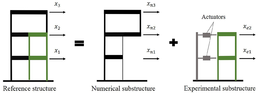
Figure 1. Real-time hybrid simulation substructuring example.

The reference structure is separated into a numerical (subscript n) and a experimental (subscript e) substructures, as shown in Equation (2):

$\begin{array}{l}(M_n+M_e)\ddot{x}(t)+(C_n+C_e)\dot{x}(t)+(K_n+K_e)x(t)\\ =-(M_n+M_e)\Gamma {\ddot{u}}_g(t)& (2)\end{array}$

Then, the EOM of the numerical substructure can be rewritten as shown in Equation (3), including the earthquake equivalent forces of the experimental substructure:

$\begin{array}{ll}{M}_n{\ddot{x}}_n(t)+C_n{\dot{x}}_n(t)+K_n{x}_n(t)=-(M_n+M_e)\Gamma {\ddot{u}}_g(t)-F_e(t)& (3)\end{array}$

where x_n(t), ẋ_n(t), and ẍ_n(t) corresponds to the displacement, velocity, and acceleration of the numerical substructure, all relative to the ground motion. Meanwhile, F_e corresponds to the feedback forces from the experimental substructure described in Equation (4):

$\begin{array}{ll}{F}_e(t)=M_e{\ddot{x}}_e(t)+C_e{\dot{x}}_e(t)+K_e{x}_e(t)& (4)\end{array}$

where x_e(t), ẋ_e(t), and ẍ_e(t) corresponds to the experimental displacement, velocity, and acceleration of the experimental substructure, and in the ideal case, the actuators imposes x_e = x_n. However, in an RTHS test, the experimental displacements are not necessarily equal to the numerical displacements due to synchronization errors introduced by the transfer system and interaction with the experimental substructure (Dyke et al., 1995).

2.2. Energy Balance

Consider that the numerical substructure is an isolated system subjected to two external forces: (i) earthquake equivalent forces; and (ii) experimental feedback forces. Assuming that an appropriate numerical integration method is implemented, so that the calculated numerical substructure response is numerically stable (Chen et al., 2009; Bas and Moustafa, 2020), the equation of motion of the numerical substructure can be expressed as an energy balance, allowing to focus the stability analysis on the interaction between hybrid substructures due to experimental errors. If numerical substructure matrices M_n, C_n, K_n are symmetric;the energy balance can be obtained by taking the inner product with an infinitesimal numerical displacement trajectory, dx_n, and then integrating both sides of Equation (3) over the displacement trajectory:

$\begin{array}{l}{\displaystyle \int }{\ddot{x}}_n^T{M}_{n}d{x}_n+{\displaystyle \int }{\dot{x}}_n^T{C}_{n}d{x}_n+{\displaystyle \int }{x}_n^T{K}_{n}d{x}_n\\ ={\displaystyle \int }-{\ddot{u}}_g{\Gamma }^T{M}_{r}d{x}_n+{\displaystyle \int }-F_e^{T}d{x}_n& (5)\end{array}$

Equation (3) can be later expressed as a scalar equation as shown in Equation (6):

$\begin{array}{ll}{E}_k+E_d+E_s=W_I+W_F& (6)\end{array}$

where E_k, E_d, and E_s are the kinetic, dissipated and strain energy of numerical substructure, respectively, as described in Equation (7):

$\begin{array}{ll}{E}_k={\displaystyle \int }{\ddot{x}}_n^T{M}_{n}d{x}_n;E_d={\displaystyle \int }{\dot{x}}_n^T{C}_{n}d{x}_n;E_s={\displaystyle \int }{x}_n^T{K}_{n}d{x}_n& (7)\end{array}$

meanwhile, W_I is the work done by the earthquake forces (namely as input work), and W_F is the work done by the experimental forces (namely as feedback work):

$\begin{array}{ll}{W}_I={\displaystyle \int }-{\ddot{u}}_g{\Gamma }^T{M}_{r}d{x}_n;W_F={\displaystyle \int }-F_e^{T}d{x}_n& (8)\end{array}$

It is worth mentioning that the energy balance from Equation (6) must be fulfilled during a test even if the experimental force is delayed, and the hybrid system is unstable. In this sense, the feedback force is just another external excitation supplied over the numerical substructure.

2.3. Proposed Stability Indicator

When a hybrid system becomes unstable, the mechanical energy of both substructures will grow exponentially even if the earthquake signal goes zero. This issue could happen if the experimental substructure introduces additional energy to the numerical substructure. Horiuchi et al. (1999) demonstrated that delay causes negative damping in the hybrid system, which is equivalent to adding external energy to the hybrid system. It is desirable to detect this problem before the mechanical energy grows up at levels that can damage the experimental equipment.

During an RTHS test, it is expected that the mechanical energy of the numerical substructure increases, because the earthquake forces introduces energy to the system, but the mechanical energy should not be greater than the input work. Reordering Equation (6) and grouping E_k and E_s in mechanical energy E_mec, Equation (9) is obtained:

$\begin{array}{ll}{W}_I-E_{mec}=E_d-W_F& (9)\end{array}$

If the feedback work, W_F, gets bigger than the dissipated energy E_d, the right side of Equation (9) becomes negative. Due to the energy balance, the left side becomes negative and indicates that mechanical energy gets bigger than the input energy. Thus, when the hybrid system's inherent dissipated energy is insufficient to counteract the added energy from the feedback force, the system will become unstable.

Therefore, the proposed analysis consists in comparing the feedback work with the dissipated energy through an indicator described in Equation (10):

$\begin{array}{ll}SW=\frac{W_F}{E_d+C_{SW}}H(W_F)·100\%& (10)\end{array}$

where SW is called the Stability Warning Indicator, and H(·) is the Heaviside function used to compute SW only when W_F is positive. Notice that the dissipated energy is always strictly positive (i.e., E_d > 0); hence, E_d − W_F could be negative only if W_F is positive. Meanwhile, C_SW is a constant chosen to prevent large values of SW when the test starts (i.e., when E_d is close to zero). Notice that E_d = 0 at t = 0 (i.e., before the earthquake starts), so C_SW should be a constant selected that is bigger enough to make the denominator to be non-zero in the SW and to prevent large values of SW if W_F is dominated by noise in the force measurements. Moreover, C_SW should be small enough, so the SW denominator would be dominated by the E_d term during and after the earthquake. As a recommendation, both conditions could be satisfied if C_SW is selected as two magnitude orders below the maximum input work over the structural system. It is worth mentioning that this input work can not be calculated before the test since the complete hybrid system's response is unknown. However, an offline estimation of the input work magnitude order is enough to select a proper C_SW.

The explanation of the SW values is provided herein. When SW = 0%, due to negative values of W_F, there is no risk of instability because the experimental substructure is removing energy from the numerical substructure. Next, if 0% < SW < 100%, the experimental substructure is adding energy; but, the damping of the numerical substructure is enough to counter this effect. Finally, if SW ≥ 100%, then the numerical substructure's mechanical energy overcomes the input work, causing instability.

The main difference between EEI and SW indicators is that the former evaluates simulation accuracy when affected by synchronization errors, and the latter is focused on assessing the stability of the hybrid system. For example, if a hybrid system presents a significant delay in the transfer system, the experimental errors will cause the experimental substructure to add energy to the numerical substructure. Nevertheless, if the numerical substructure has enough damping to maintain the system stable, the SW will be <100%; meanwhile, EEI will show large values due to the synchronization errors produced by the delay.

3. Numerical Application

3.1. Benchmark Problem

The virtual RTHS benchmark problem from Silva et al. (2020) is considered as a practical example to prove the capacity of the proposed indicator to detect instability. This problem consists of a three-story moment frame with three lateral degrees of freedom as the reference structure (see Figure 2). This structure is separated into a 3DOF numerical substructure and an SDOF experimental substructure.

FIGURE 2

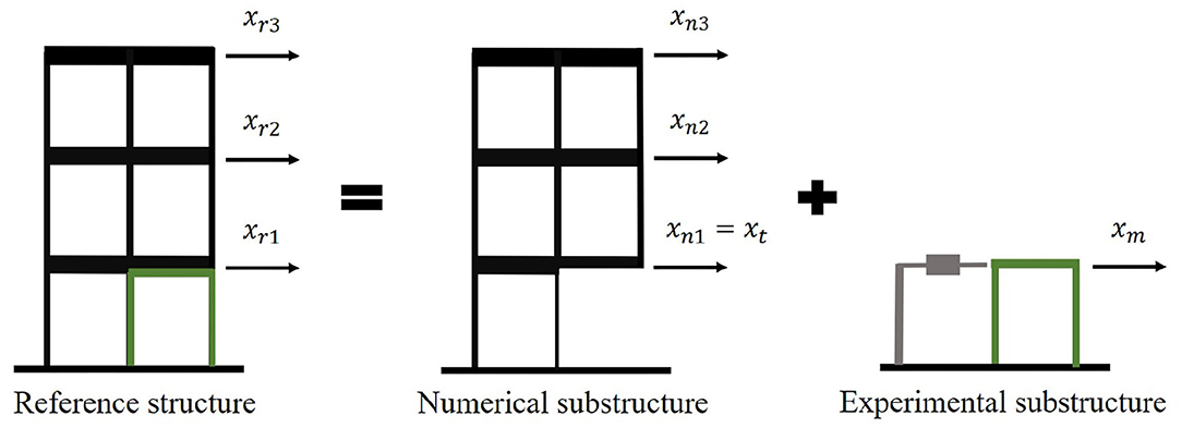
Figure 2. Reference structure and partitioning.

The reference structure properties are: mass per floor m = 1, 000 kg; natural frequencies f = [3.61, 16.00, 38.09] Hz; and modal damping ζ = 3% for each mode. These properties corresponds to Case IV from Silva et al. (2020). The reference structure is partitioned as described in Equation (11):

$\begin{array}{ll}{M}_r=M_n+M_e;C_r=C_n+C_e;K_r=K_n+K_e& (11)\end{array}$

where M_e = diag(m_e, 0, 0); C_e = diag(c_e, 0, 0); and K_e = diag(k_e, 0, 0). The structural properties of the experimental substructure are m_e = 29.1 kg; c_e = 114.6 Nsec/m; and $k_e=1.19\times 10^6$ N/m.

The reference structure and the numerical substructure are implemented in the state-space form using Simulink for direct integration. The solver utilized is a 4th Order Runge-Kutta with a fixed time step of Δt = 1/4, 096 s. The reference structure model is presented in Equations (12) and (13) with ground acceleration as input and reference displacements as output.

$\begin{array}{ll}\left\{\begin{array}{c}{\dot{x}}_r\\ {\ddot{x}}_r\end{array}\right\}=\left[\begin{array}{cc}0& I\\ -M_r^{-1}{K}_r& -M_r^{-1}{C}_r\end{array}\right]\left\{\begin{array}{c}{x}_r\\ {\dot{x}}_r\end{array}\right\}+\left[\begin{array}{c}0\\ -\Gamma \end{array}\right]\left\{\begin{array}{c}{\ddot{u}}_g\end{array}\right\}& (12)\end{array}$

$\begin{array}{ll}\left\{\begin{array}{c}{x}_r\end{array}\right\}=\left[\begin{array}{cc}I& 0\end{array}\right]\left\{\begin{array}{c}{x}_r\\ {\dot{x}}_r\end{array}\right\}+\left[\begin{array}{c}0\end{array}\right]\left\{\begin{array}{c}{\ddot{u}}_g\end{array}\right\}& (13)\end{array}$

The numerical substructure model is presented in Equations (14) and (15) with ground acceleration and experimental force as inputs and numerical displacements, velocities, and accelerations as outputs.

$\begin{array}{ll}\left\{\begin{array}{c}{\dot{x}}_n\\ {\ddot{x}}_n\end{array}\right\}=\left[\begin{array}{cc}0& I\\ -M_n^{-1}{K}_n& -M_n^{-1}{C}_n\end{array}\right]\left\{\begin{array}{c}{x}_n\\ {\dot{x}}_n\end{array}\right\}+\left[\begin{array}{cc}0& 0\\ -M_n^{-1}{M}_r\Gamma & -M_n^{-1}\gamma \end{array}\right]\left\{\begin{array}{c}{\ddot{u}}_g\\ f_e\end{array}\right\}& (14)\end{array}$

$\begin{array}{ll}\left\{\begin{array}{c}{x}_n\\ {\dot{x}}_n\\ {\ddot{x}}_n\end{array}\right\}=\left[\begin{array}{cc}I& 0\\ 0& I\\ -M_n^{-1}{K}_n& -M_n^{-1}{C}_n\end{array}\right]\left\{\begin{array}{c}{x}_n\\ {\dot{x}}_n\end{array}\right\}+\left[\begin{array}{cc}0& 0\\ 0& 0\\ -M_n^{-1}{M}_r\Gamma & -M_n^{-1}\gamma \end{array}\right]\left\{\begin{array}{c}{\ddot{u}}_g\\ f_e\end{array}\right\}& (15)\end{array}$

where γ = [1;0;0]^T and f_e is experimental force calculated as shown in Equation (16):

$\begin{array}{ll}{f}_e=k_e{x}_m+c_e{\dot{x}}_m+m_e{\ddot{x}}_m& (16)\end{array}$

and x_m, ẋ_m, and ẍ_m are the measured displacement, velocity and acceleration imposed on the experimental substructure.

To compute the Stability Warning Indicator (SW) it is necessary to evaluate different energy terms using numerical integration. To calculate the accumulated energy E[j] of a force P[i] over a displacement increment Δx[i], ∀i ∈ [1, j], a trapezoidal rule is formulated in Equation (17):

$\begin{array}{ll}E\left[j\right]={\displaystyle \sum _{i=1}^j}\frac{1}{2}(P\left[i\right]+P\left[i-1\right])(x\left[i\right]-x\left[i-1\right])& (17)\end{array}$

This integration method is implemented in Simulink, as shown in the block diagram of Figure 3, where Discrete Finite Impulse Response (FIR) Filters and Product blocks are employed to obtain the area of each trapezoid, and a Discrete-time Integrator block is required to obtain the accumulation over time. In the case of W_F the input force is P = f_e and the input displacement is $x=x_n^{(1)}$ (scalar signals); meanwhile, to evaluate E_d, the input forces are P = C_nẋ_n and the displacements are x = x_n (vector signals).

FIGURE 3

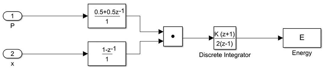
Figure 3. Block diagram for energy calculation.

Additionally, to compare the proposed stability indicator, the EEI (Ahmadizadeh and Mosqueda, 2009) is calculated for each simulation. The EEI can be obtained as follow:

$\begin{array}{ll}EEI=\frac{W_I-(E_k^{*}+E_d^{*}+E_s-W_{exp})}{W_I+E_E^{max}}& (18)\end{array}$

where $E_k^{*}$, $E_d^{*}$ are the kinetic and dissipated energy calculated with the first derivative of displacement instead of velocity of numerical substructure. $E_E^{max}$ is a nonzero elastic energy term utilized to normalize EEI when W_I is close to zero at the beginning of the test. It is important to declare that non-compensated delay implies added energy to the system, resulting in negative values of EEI. W_exp is the work done by experimental force over the measured displacement as shown in Equation (19):

$\begin{array}{ll}{W}_{exp}={\displaystyle \int }-f_e^{T}d{x}_m& (19)\end{array}$

In this study, the reference structure is subjected to the Kobe earthquake with a peak ground acceleration (PGA) scaled to 40%, and the maximum input work from the earthquake is around 100 Joules. This value can be computed from the integration of the reference structure. In a real RTHS experiment, the magnitude order of the input energy can be estimated from the ground motion and global properties of the structure, such as total mass and approximated damping and stiffness. Therefore, the denominator constants are selected considerably smaller, such as 1% of the maximum input work:

$\begin{array}{ll}{E}_E^{max}=C_{SW}=1\text{ Joule}& (20)\end{array}$

This value is bigger enough to prevent large values for each indicator at the beginning of the earthquake. Also, these constants will have a negligible effect on each indicator during and after the earthquake, since C_SW will be relatively small compared with E_d in the denominator of Equation (10), just like $E_E^{max}$ will be smaller than W_I in the denominator of Equation (18).

3.2. Critical Delay Estimation

Before conducting the RTHS simulations with different delay values, an estimation of the critical delay is obtained with the method proposed by Gao and You (2019). This method consists in constructing the EOM of the hybrid system with some assumptions synchronization errors (delay and amplitude errors). The EOM of the hybrid system has the following equivalent mass, damping, and stiffness:

$\begin{array}{ll}{M}_{eq}=M_n\Phi {\Phi }^{-1}+M_e\Phi \Delta {\Phi }^{-1}-C_e\Phi \Delta \delta {\Phi }^{-1}& (21)\end{array}$

$\begin{array}{ll}{C}_{eq}=C_n\Phi {\Phi }^{-1}+M_e\Phi \Delta {\omega }^2\delta {\Phi }^{-1}+C_e\Phi \Delta {\Phi }^{-1}-K_e\Phi \Delta \delta {\Phi }^{-1}& (22)\end{array}$

$\begin{array}{ll}{K}_{eq}=K_n\Phi {\Phi }^{-1}+K_e\Phi \Delta {\Phi }^{-1}& (23)\end{array}$

where Φ is the modal matrix of the reference system, ω is a diagonal matrix with the natural frequencies of the reference system, δ is a diagonal matrix with the delay for each mode, and Δ is a diagonal matrix with the amplitude error for each mode. With the equivalent properties of the hybrid system, the state matrix A_eq is constructed as shown in Equation (24):

$\begin{array}{ll}{A}_{eq}=\left[\begin{array}{cc}0& I\\ -M_{eq}^{-1}{K}_{eq}& -M_{eq}^{-1}{C}_{eq}\end{array}\right]& (24)\end{array}$

The hybrid system is stable if the matrix A_eq has eigenvalues with negative real part; thus, the critical delay can be obtained by searching the minimum constant delay that produces eigenvalues with positive real part. For the partitioning of this problem, assuming Δ = I and δ = diag(τ_cr; τ_cr; τ_cr), the critical delay is:

$\begin{array}{ll}{\tau }_{cr}=8.5\text{ msec}& (25)\end{array}$

This critical delay serves as a reference for the simulations with constant delay. It is expected that simulations with delays smaller than this critical value would remain stable while running the simulations. In contrast, the opposite will result in an unstable response.

4. Results

4.1. RTHS With Constant Delay

The Simulink block diagram for the simulations with constant delay is presented in Figure 4, where the output of the numerical substructure, denoted as “target vector,” is defined as $x_t={\left[x_n^{(1)};{\dot{x}}_n^{(1)};{\ddot{x}}_n^{(1)}\right]}^T$ (displacement, velocity and acceleration of first degree of freedom). Then, the Delay block generates a discrete delay of the input signal x_t by a specified number of samples d, so the time delay τ is a multiple of the simulation time step. Then, the delayed boundary conditions are:

$\begin{array}{ll}{x}_d={\left[x_n^{(1)}(t-\tau );{\dot{x}}_n^{(1)}(t-\tau );{\ddot{x}}_n^{(1)}(t-\tau )\right]}^T& (26)\end{array}$

Finally, the outputs of experimental substructure are described in Equations (27) and (28):

$\begin{array}{ll}{x}_m=x_n^{(1)}(t-\tau )& (27)\end{array}$

$\begin{array}{ll}{f}_e=\left[k_e;c_e;m_e\right]x_d& (28)\end{array}$

Four simulations are performed with different delay values from 0 to 9 ms. The structure is subjected to the Kobe earthquake with a peak ground acceleration (PGA) scaled to 40%. The measured displacement of experimental substructure x_m is compared with the first degree of freedom displacement x_r1 from the reference structure, as shown in Figure 5. Measured displacements are very close to reference displacements for lower values of delay (τ = 0 ms and τ = 0.98 ms). Then, for higher delay τ = 7.1 ms, a notorious synchronization error in displacements appear, but at least the measured displacement decays at the end of the simulation. This does not happen with τ = 9msec > τ_cr, where the measured displacement grows exponentially after the earthquake reaches zero.

FIGURE 4

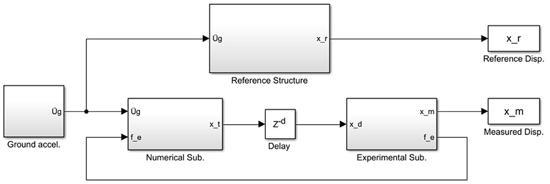
Figure 4. Reference structure and RTHS partitioning with delay.

FIGURE 5

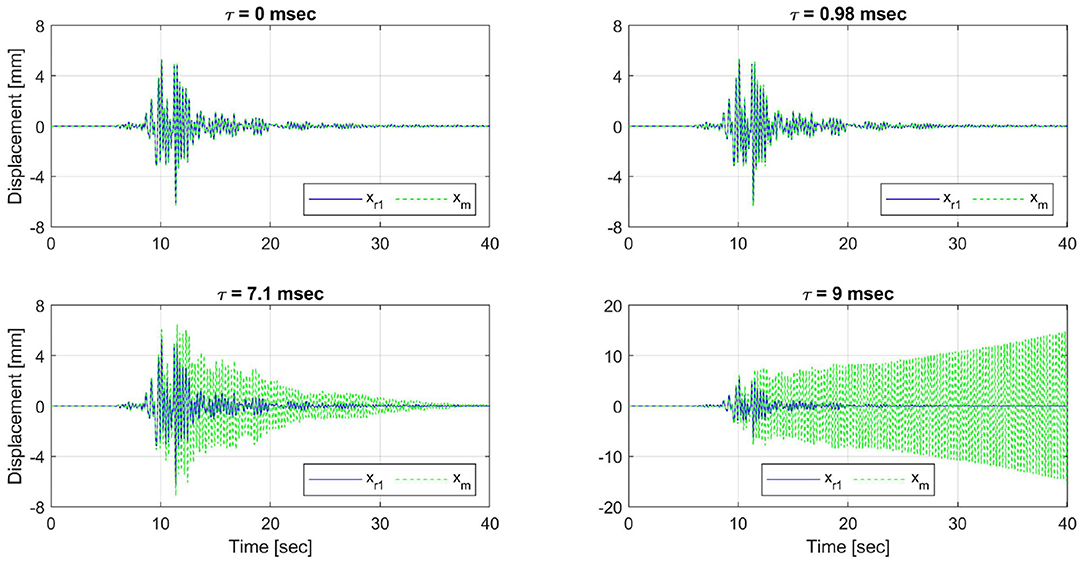
Figure 5. Reference and measured displacements for different delay values.

In Figure 6, the error of displacement x_m respect to x_r1 for each delay is presented, including the normalized root mean square error (NRMSE) for each case. Clearly, for τ = 0 ms and τ = 0.98 ms, the system is stable; while, for τ = 9 ms is unstable (i.e., error grows exponentially). However, for τ = 7.1 ms, the error is considerable, with NRSME = 144%, but the system is still stable. It is easy to classify the case with τ = 9 ms as unstable after the test. Still, it would be beneficial to detect unstable behavior before the system reaches a large response.

FIGURE 6

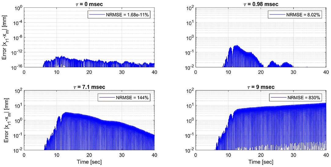
Figure 6. Displacement error for different delay values.

In Figure 7, the SW indicator is calculated for each model scenario. For τ = 0 ms, τ = 0.98 ms, and τ = 7.1 ms, the indicator stays under 100% during the entire test, showing the stable behavior of each simulation. In contrast, for the unstable case with τ = 9 ms, the indicator exceeds 100% near 10 s of simulation, much earlier than the instant when the system reaches the large displacements presented in Figure 5. Thus, the SW indicator could help stop the simulation in time, avoiding any dangerous behavior in the RTHS test.

FIGURE 7

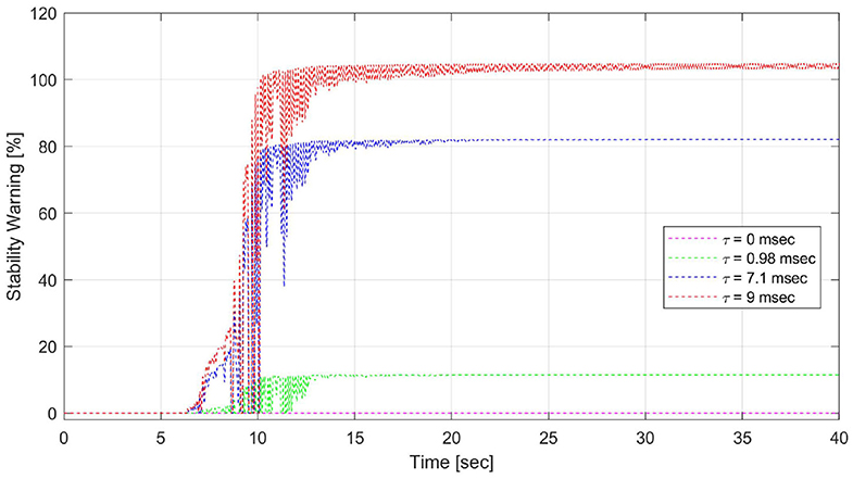
Figure 7. Stability warning indicator (SW) for different delay values.

For the sake of comparison, Figure 8 shows the absolute value of EEI for each case scenario. The EEI grows up with higher values of delay but is not evident in which case is stable and in which it is not. For τ = 0 ms, the EEI values are relatively small. Moreover, for τ = 0.98 ms, the EEI stays under 15% during the test; both cases are indeed stable. However, for τ = 7.1 ms, the behavior of EEI is similar to τ = 9 ms before 15 s of simulation, so it is not possible to detect instability until the earthquake signal dies out. If the EEI is utilized to stop unstable testing, it is quite challenging to define a threshold that relates EEI with instability. For example, for a threshold of EEI = 100%, the simulations with τ = 7.1 ms and τ = 9 ms should be stopped before 10 sec, even when the simulation with τ = 7.1 ms is stable and does not present any risk of large displacements. Nevertheless, it must be recognized that EEI is an excellent tool to assess the accuracy of the results from an RTHS test through a post-processing analysis.

FIGURE 8

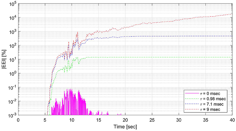
Figure 8. Energy error indicator (EEI) for different delay values.

4.2. RTHS With Actuator Model and Dynamic Compensation

In this subsection, the same partitioning as in the previous subsection is utilized, but in this case a transfer system is modeled as presented in Silva et al. (2020), and adaptive compensation with different design parameters is implemented to minimize the errors produced by the transfer system. The block diagram utilized to model this problem in Simulink is presented in Figure 9, where the output of the numerical substructure is the target displacement $x_t=x_n^{(1)}$ (displacement of first degree of freedom). Then, the target displacement is sent to the adaptive controller to determine the commanded displacement for the actuator. The plant (i.e., actuator connected to the experimental substructure) is modeled with the transfer function presented in Equation (29), which includes actuators parameters and interaction with the experimental substructure, and relates the commanded displacement x_c with the measured displacement x_m:

FIGURE 9

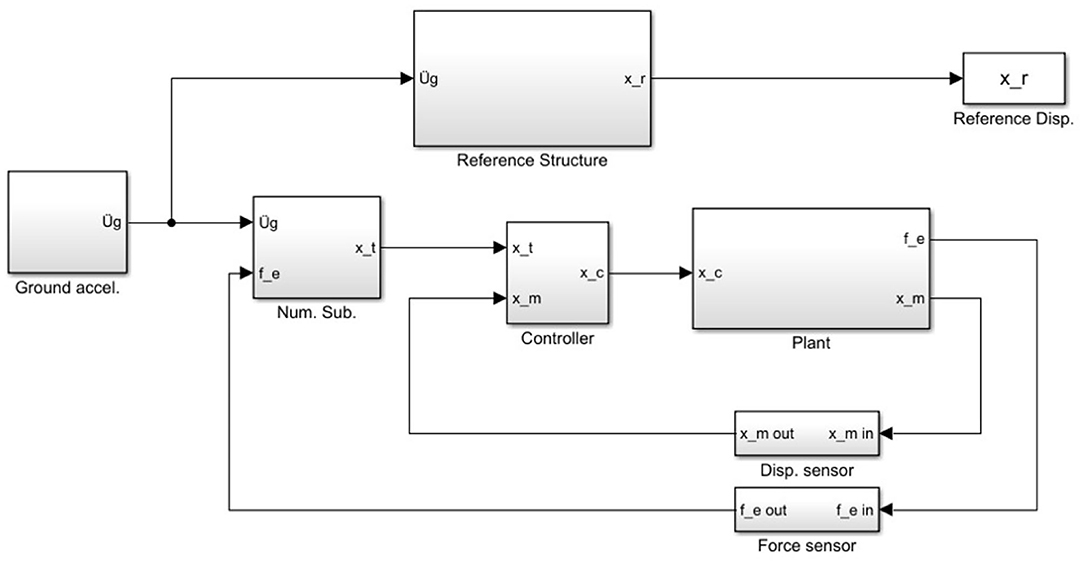
Figure 9. Reference structure and RTHS with compensation.

$\begin{array}{ll}{x}_m=\frac{2.19\times 10^{13}}{(29.1)s^5+(1.26\times 10^4)s^4+(8.42\times 10^6)s^3+(2.33\times 10^9)s^2+(5.44\times 10^{11})s+(2.17\times 10^{13})}{x}_c& (29)\end{array}$

where s = iω, is the Laplace variable, i is the complex number and ω is the circular frequency. This transfer function has a frequency-dependent phase. The phase is another way to state that the measured and commanded displacements are delayed. Thus, the delay is frequency-dependent for stable and underdamped linear systems.

The interaction forces are obtained with Equation (30):

$\begin{array}{ll}{f}_e=(m_e{s}^2+c_{e}s+k_e)x_m& (30)\end{array}$

Besides, sensor noise has been added to the measured displacement x_m and the experimental force f_e using band-limited white noise (BLWN) blocks to model the physical sensors. Then, the signal x_m is sent to the controller for the adaptation process. Consequently, the signal f_e is fed back to the numerical substructure to be considered in the integration of the numerical EOM. Notice that force measurement noise could impact the experimental force power, but it has a small effect on the work done by this force due to the numerical integration process to calculate work. However, measurement noises can affect the hybrid loop, depending on the structural properties, transfer system, and dynamic compensation.

The adaptive compensation implemented in the controller consist in adaptive model-based compensation (Chen et al., 2015) with the modifications presented in Fermandois et al. (2020). A first-order adaptive feedforward determines the commanded displacement as shown in Equation (31):

$\begin{array}{ll}{x}_c=a_0{x}_t+a_1{\dot{x}}_t& (31)\end{array}$

where a₀ and a₁ are the adaptive control parameters, and ẋ_t is approximated using the backwards difference method. The adaptation laws of a₀ and a₁ are described in Equation (32):

$\begin{array}{ll}\left\{\begin{array}{c}{\dot{a}}_0\\ {\dot{a}}_1\end{array}\right\}=\Gamma e\left\{\begin{array}{c}{x}_m\\ {\dot{x}}_m\end{array}\right\}& (32)\end{array}$

where Γ = diag(Γ₀, Γ₁) is the adaptive gain matrix associated with the adaptation rate of parameters a₀ and a₁, respectively, and e is an estimation error of the adaptive parameters described in Equation (33):

$\begin{array}{ll}e=\frac{x_c-(a_0{x}_m+a_1{\dot{x}}_m)}{1+(x_m^2+{\dot{x}}_m^2)}& (33)\end{array}$

Both signals x_c and x_m are filtered with a fourth-order Butterworth low-pass filter with a cutoff frequency of 20 Hz, and ẋ_m is obtained with the backward difference method.

This subsection aims to demonstrate the performance of the SW stability indicator for different compensation scenarios. Notice that the goal of the SW indicator is to detect instability during a test with a predefined compensation design, and not to tune the compensation/adaptation parameters. In these simulations, the initial adaptive parameters are selected as a₀(t = 0) = 1 and a₁(t = 0) = 10/1, 000 s. With these parameters, the controller cannot compensate for the control plant delay successfully; therefore, parameter adaptation is necessary.

Four simulations are performed with different adaptive gains presented in Table 1, where Γ_a corresponds to a non-adaptive case, Γ_d to an optimally calibrated case (Fermandois et al., 2020), and Γ_b and Γ_c are intermediate cases of adaptation. The structure is subjected to the Kobe earthquake scaled to 40% PGA.

TABLE 1

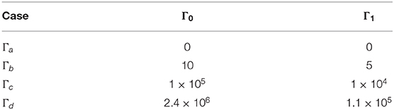
Table 1. Adaptive gains for each case.

The measured displacement of experimental substructure x_m is compared with the first degree of freedom displacement x_r1 from the reference structure in Figure 10, where the case with Γ_a is unstable, while the case with Γ_b presents large measured displacements, but that decreases after the earthquake. Considering that in true RTHS tests, the reference displacement is not available, it would be difficult to distinguish if the measured displacements are correct or are associated with an unstable response. On the other hand, for Γ_c and Γ_d simulations are stable. In Figure 11, the error of displacement x_m respect to x_r1 for each adaptive gains is presented, including the normalized root mean square error (NRMSE) for each case. The cases with Γ_a present unacceptable errors, while for Γ_b, the errors are substantial, but at least decrease after the earthquake. For the cases with Γ_c and Γ_d, the errors are relatively small.

FIGURE 10

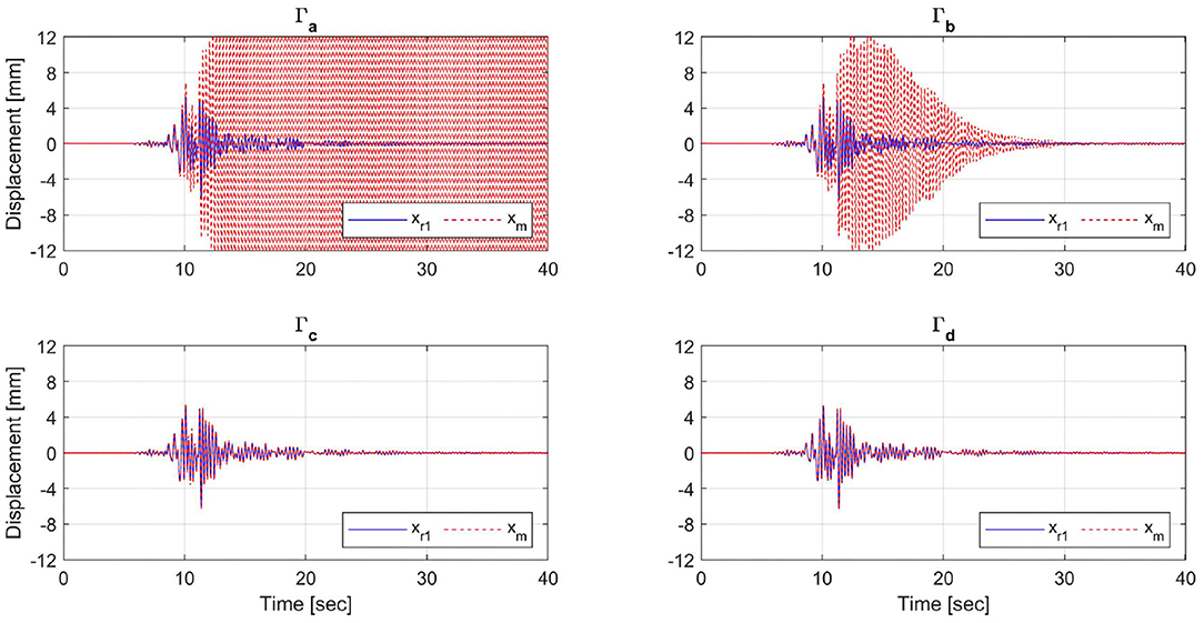
Figure 10. Reference and measured displacements for different adaptive gains.

FIGURE 11

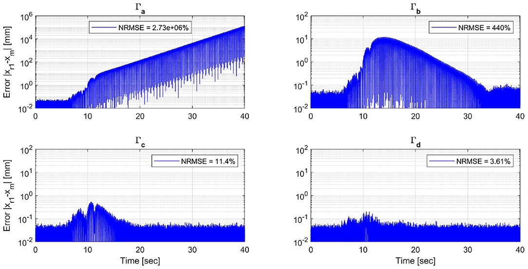
Figure 11. Displacement error for different adaptive gains.

The difference between each case is explained by the adaptation process presented in Figure 12, where there is no adaptation for Γ_a, slow adaptation for Γ_b, and the same convergence for Γ_c and Γ_d but with different rates. The parameter a₁ is directly related to the delay compensation, so it is expected that for Γ_a and Γ_b, the non-compensated delay produces large errors in the simulations. However, the adaptation for Γ_b is apparently enough to stabilize the system during the test.

FIGURE 12

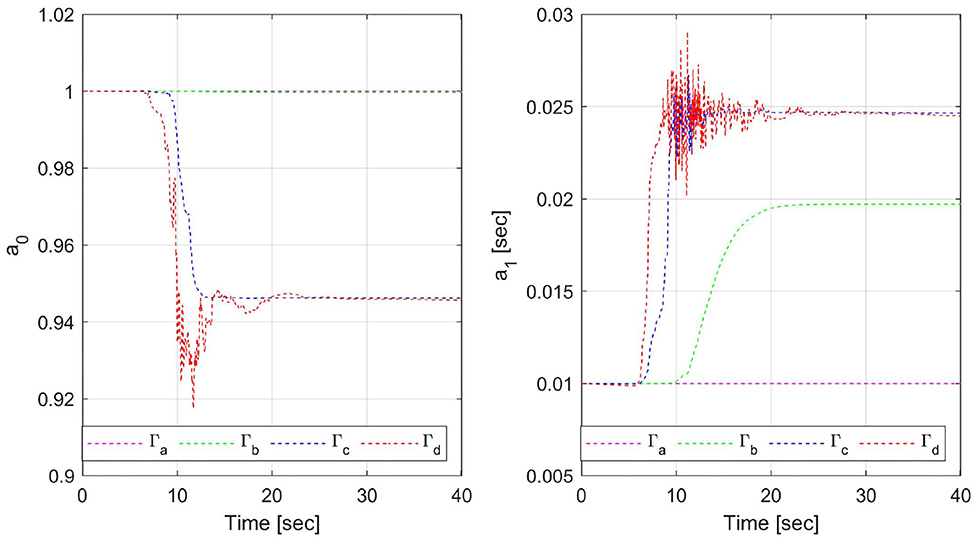
Figure 12. Adaptation of control parameters a₀ and a₁ for different adaptive gains.

In Figure 13, the SW indicator for each case is presented. For Γ_c and Γ_d, the indicator is growing at the beginning of the earthquake. Then, the SW indicator decays due to the adaptation and good compensation, and stays under 100% during the entire simulation, confirming the stability of these simulations. For Γ_a and Γ_b, the indicator reaches 100% near 10 s of simulation, so much before each simulation presents large displacements. So, the stability warning indicator could help stop the simulation in time before any damage occurs in the test setup. In the particular case with Γ_b, the stability warning indicator exceeds 100% between 10 and 20 s, consistent with the large response of the system in that interval. After 20 s of simulation, when the controller has reached enough adaptation to compensate for the delay, the SW indicator decays below 100%. This result is consistent with the stable behavior of this case at the end of the simulation. However, this simulation could be stopped when the indicator reaches 100% to avoid the behavior shown between 10 and 20 s.

FIGURE 13

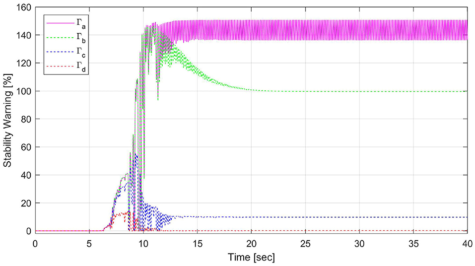
Figure 13. Stability warning indicator (SW) for different adaptive gains.

Moreover, notice that for Γ_b and Γ_c cases, the SW does not decay to zero at the end of the simulation. This situation occurs because of uncompensated delay during the earthquake, which causes a surplus of energy inserted into the numerical substructure. Later, when the delay is compensated, displacements and forces are too small, so the work done by the experimental forces remains constant. This effect does not happen for Γ_d, where the delay is compensated early when the earthquake strikes. The experimental substructure dissipates energy during the rest of the earthquake, leading W_F to zero and consequently, SW to zero as well.

Furthermore, the control plant in the benchmark problem is modeled as a linear time-invariant system, but in these simulations, the adaptive controller produces time-varying compensation. Therefore, the delay between target and measured displacements is a time-varying property. This scenario is a complicated situation to predict the stability of a system before the test. However, with the online analysis of the SW it is possible to detect which case results in stable behavior and which are not.

For comparison, Figure 14 shows the absolute value of EEI for each adaptive case scenario. For Γ_a and Γ_b, the EEI presents large values, while for Γ_d, the EEI keeps low during the test. So, the EEI could allow lab technicians to stop the simulations with Γ_a and Γ_b, and accept the simulation with Γ_d. However, for Γ_c case, the EEI reaches 100% before 10 s where the displacements are small, and the controller is adapting, and the test still has good chance to give acceptable results without the risk of instability. Thus, the EEI is an excellent tool to analyze the errors after the RTHS test, but it is not reliable for detecting instability online.

FIGURE 14

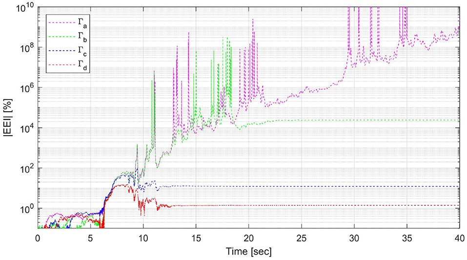
Figure 14. Energy error indicator (EEI) for different adaptive gains.

Additionally, in these simulations, displacement and force measurement noises do not have a notorious impact on the hybrid system response. The numerical substructure acts like a low-pass filter for the force measurement, and the adaptive compensator is not affected by the displacement noise.

5. Conclusions

Energy analysis for real-time hybrid simulation tests is conducted to establish a stability indicator for online evaluation. The features of the proposed indicator to detect instability is demonstrated through numerical simulations with constant delay, including an actuator model with adaptive compensation for different design scenarios. The stability warning indicator (SW) allows the detection of unstable behavior before the system reaches large displacements that can damage the experimental substructure or laboratory equipment. The proposed indicator only requires the measured force from the experimental substructure and information from the numerical substructure. Hence, it is independent of the compensation method and does not require a model of the experimental substructure or the transfer system (i.e., actuation system). This indicator can be implemented to stop an RTHS test that is rendered unstable automatically. The test should be stopped if the SW reaches 100% (i.e., it is unnecessary to stop a test with a SW < 100). So, this indicator is an excellent complement to any compensation method. It provides further safety guarantees to the test, especially for adaptive compensation if there is considerable uncertainty in the plant or the controller's adaptation capacity. It is worth mentioning that the proposed indicator provides safety for the test, but it does not ensure accuracy compared to the reference structure's true response. However, priority should always be given to conducting a safe experiment. Then, the reliability of the results could be studied in detail after the test has ended.

Finally, the effectiveness of the SW indicator is demonstrated for linear systems. Future work will consider non-linear systems and the corresponding experimental validation of the proposed indicator, together with the implementation of existing compensation techniques in RTHS testing and its synergism.

Data Availability Statement

All datasets generated for this study are included in the article/supplementary material.

Author Contributions

CG and GF conceived the presented idea for this study. CG developed the methodology and performed the numerical simulations. GF supervised the findings of this work. CG wrote the manuscript with support from GF. All authors discussed the results and contributed to the final manuscript.

Conflict of Interest

The authors declare that the research was conducted in the absence of any commercial or financial relationships that could be construed as a potential conflict of interest.

Acknowledgments

The authors gratefully acknowledge the financial support from the Universidad Técnica Federico Santa María (Chile) through the research grant Proyecto Interno de Línea de Investigación No. PI_L_18_07, and from the Chilean National Commission for Scientific and Technological Research (CONICYT), FONDECYT Iniciación Research Project, Grant No. 11190774. The authors' opinions, findings, conclusions, or recommendations are those of the authors and do not necessarily reflect those of the sponsors.

References

Ahmadizadeh, M., and Mosqueda, G. (2009). Online energy-based error indicator for the assessment of numerical and experimental errors in a hybrid simulation. Eng. Struct. 31, 1987–1996. doi: 10.1016/j.engstruct.2009.03.002

CrossRef Full Text | Google Scholar

Bas, E. E., and Moustafa, M. A. (2020). Performance and limitations of real-time hybrid simulation with nonlinear computational substructures. Exp. Tech. doi: 10.1007/s40799-020-00385-6

CrossRef Full Text | Google Scholar

Bonnet, P. A., Lim, C. N., Williams, M. S., Blakeborough, A., Neild, S. A., Stoten, D. P., et al. (2007). Real-time hybrid experiments with Newmark integration, MCSmd outer-loop control and multi-tasking strategies. Earthq. Eng. Struct. Dyn. 36, 119–141. doi: 10.1002/eqe.628

CrossRef Full Text | Google Scholar

Carrion, J. E., and Spencer, B. F. (2007). Model-Based Strategies for Real-Time Hybrid Testing. Technical Report NSEL-006, Department of Civil and Environmental Engineering, University of Illinois at Urbana-Champaign, Urbana, IL.

Google Scholar

Chae, Y., Kazemibidokhti, K., and Ricles, J. M. (2013). Adaptive time series compensator for delay compensation of servo-hydraulic actuator systems for real-time hybrid simulation. Earthq. Eng. Struct. Dyn. 42, 1697–1715. doi: 10.1002/eqe.2294

CrossRef Full Text | Google Scholar

Chen, C., Ricles, J. M., Marullo, T. M., and Mercan, O. (2009). Real-time hybrid testing using the unconditionally stable explicit CR integration algorithm. Earthq. Eng. Struct. Dyn. 38, 23–44. doi: 10.1002/eqe.838

CrossRef Full Text | Google Scholar

Chen, P.-C., Chang, C.-M., Spencer, B. F. Jr., and Tsai, K.-C. (2015). Adaptive model-based tracking control for real-time hybrid simulation. Bull. Earthq. Eng. 13, 1633–1653. doi: 10.1007/s10518-014-9681-2

CrossRef Full Text | Google Scholar

Dyke, S. J., Gomez, D., and Spencer, B. F. (2020). Editorial: Special issue on the real-time hybrid simulation benchmark problem. Mech. Syst. Signal Process. 142:106804. doi: 10.1016/j.ymssp.2020.106804

CrossRef Full Text | Google Scholar

Dyke, S. J., Spencer, B. F. Jr., Quast, P., and Sain, M. (1995). Role of control-structure interaction in protective system design. J. Eng. Mech. 121, 322–338. doi: 10.1061/(ASCE)0733-9399(1995)121:2(322)

CrossRef Full Text | Google Scholar

Fermandois, G., Galmez, C., and Valdebenito, M. (2020). “Optimal gain calibration of adaptive model-based compensation for real-time hybrid simulation testing,” in 17th World Conference on Earthquake Engineering (17WCEE) (Sendai).

Google Scholar

Gao, X., Castaneda, N., and Dyke, S. J. (2013). Real time hybrid simulation: from dynamic system, motion control to experimental error. Earthq. Eng. Struct. Dyn. 42, 815–832. doi: 10.1002/eqe.2246

CrossRef Full Text | Google Scholar

Gao, X. S., and You, S. (2019). Dynamical stability analysis of MDOF real-time hybrid system. Mech. Syst. Signal Process. 133:106261. doi: 10.1016/j.ymssp.2019.106261

CrossRef Full Text | Google Scholar

Guo, T., Chen, C., Xu, W., and Sanchez, F. (2014). A frequency response analysis approach for quantitative assessment of actuator tracking for real-time hybrid simulation. Smart Mater. Struct. 23:045042. doi: 10.1088/0964-1726/23/4/045042

CrossRef Full Text | Google Scholar

Horiuchi, T., Inoue, M., Konno, T., and Namita, Y. (1999). Real-time hybrid experimental system with actuator delay compensation and its application to a piping system with energy absorber. Earthq. Eng. Struct. Dyn. 28, 1121–1141. doi: 10.1002/(SICI)1096-9845(199910)28:10<1121::AID-EQE858>3.0.CO;2-O

CrossRef Full Text | Google Scholar

Maghareh, A., Dyke, S., Rabieniaharatbar, S., and Prakash, A. (2017). Predictive stability indicator: a novel approach to configuring a real-time hybrid simulation. Earthq. Eng. Struct. Dyn. 46, 95–116. doi: 10.1002/eqe.2775

CrossRef Full Text | Google Scholar

McCrum, D., and Williams, M. (2016). An overview of seismic hybrid testing of engineering structures. Eng. Struct. 118, 240–261. doi: 10.1016/j.engstruct.2016.03.039

CrossRef Full Text | Google Scholar

Mercan, O., and Ricles, J. M. (2008). Stability analysis for real-time pseudodynamic and hybrid pseudodynamic testing with multiple sources of delay. Earthq. Eng. Struct. Dyn. 37, 1269–1293. doi: 10.1002/eqe.814

CrossRef Full Text | Google Scholar

Nakashima, M., Kato, H., and Takaoka, E. (1992). Development of real-time pseudo dynamic testing. Earthq. Eng. Struct. Dyn. 21, 79–92. doi: 10.1002/eqe.4290210106

CrossRef Full Text | Google Scholar

Palacio-Betancur, A., and Gutierrez Soto, M. (2019). Adaptive tracking control for real-time hybrid simulation of structures subjected to seismic loading. Mech. Syst. Signal Process. 134:106345. doi: 10.1016/j.ymssp.2019.106345

CrossRef Full Text | Google Scholar

Silva, C. E., Gomez, D., Maghareh, A., Dyke, S. J., and Spencer, B. F. (2020). Benchmark control problem for real-time hybrid simulation. Mech. Syst. Signal Process. 135:106381. doi: 10.1016/j.ymssp.2019.106381

CrossRef Full Text | Google Scholar

Tao, J., and Mercan, O. (2019). A study on a benchmark control problem for real-time hybrid simulation with a tracking error-based adaptive compensator combined with a supplementary proportional-integral-derivative controller. Mech. Syst. Signal Process. 134:106346. doi: 10.1016/j.ymssp.2019.106346

CrossRef Full Text | Google Scholar

Wallace, M., Sieber, J., Neild, S. A., Wagg, D. J., and Krauskopf, B. (2005a). Stability analysis of real-time dynamic substructuring using delay differential equation models. Earthq. Eng. Struct. Dyn. 34, 1817–1832. doi: 10.1002/eqe.513

CrossRef Full Text | Google Scholar

Wallace, M., Wagg, D., and Neild, S. (2005b). An adaptive polynomial based forward prediction algorithm for multi-actuator real-time dynamic substructuring. Proc. R. Soc. A Math. Phys. Eng. Sci. 461, 3807–3826. doi: 10.1098/rspa.2005.1532

CrossRef Full Text | Google Scholar

Wang, Z., Ning, X., Xu, G., Zhou, H., and Wu, B. (2019). High performance compensation using an adaptive strategy for real-time hybrid simulation. Mech. Syst. Signal Process. 133:106262. doi: 10.1016/j.ymssp.2019.106262

CrossRef Full Text | Google Scholar

Xu, D., Zhou, H., Shao, X., and Wang, T. (2019a). Performance study of sliding mode controller with improved adaptive polynomial-based forward prediction. Mech. Syst. Signal Process. 33:106263. doi: 10.1016/j.ymssp.2019.106263

CrossRef Full Text | Google Scholar

Xu, W., Chen, C., Guo, T., and Chen, M. (2019b). Evaluation of frequency evaluation index based compensation for benchmark study in real-time hybrid simulation. Mech. Syst. Signal Process. 130, 649–663. doi: 10.1016/j.ymssp.2019.05.039

CrossRef Full Text | Google Scholar