Delft3D as a Tool for Living Shoreline Design Selection by Coastal Managers

Introduction

Around the globe, many estuarine basins are adjusting morphologically to maintain equilibrium with sea level rise (Morris et al., 2002; Passeri et al., 2015). Their adjustment often results in increases in depth or width to inlets, changes to tidal prism, shoreline erosion, and changes to aquatic species communities (Hoyt, 1967; White et al., 2006; Huff and Feagin, 2017). A common mitigating response is placement of erosion reduction structures such as sea walls, sand engines, or living shorelines (Williams et al., 2018). However, selection of the appropriate structure is a complex task that requires extensive knowledge of system dynamics.

One wave abatement structure that has gained popularity has been the living shoreline (Miller et al., 2016; Smith et al., 2020). This building concepts seeks to balance erosion control with long term habitat and sediment management goals. Often living shorelines are constructed in a manner to promote self healing and vertical accretion by the continued growth of oysters. Weaver et al. (2017) outlined eight ecosystem services living shorelines can provide: sediment accretion, self healing, improved water quality, improved carbon sequestration, refuge habitat, improved recreational and commercial fishing, wave energy reduction, and improved durability and resiliency over traditional structures during tropical events. These concepts have further been supported by Smith et al. (2020) and Smith (2006).

Modern management goals for living shorelines often dictate that such structures must provide aquatic habitat, reduce sediment loss through scouring, allow for safe navigation, and reduce shoreline erosion (Vona et al., 2021). Moreover, they can be expensive to construct and demand extensive input from stakeholders to appropriately balance objectives (Cooper and McKenna, 2008; Williams et al., 2018). Delft3D gives scientists a tool to quickly test potential erosion abatement designs using computer modeling. Created by Deltares, Delft3D has proven to be a powerful tool for modeling estuarine flow behavior (Elias et al., 2000; Sutherland et al., 2004). One of its more recent upgrades includes the option of flexible meshes (Deltares Flexible Mesh Suite HM 2021.03) (Delft3D [computer software], 2021) which was utilized in this study. This software allows for the flexibility to work at various spatial resolutions and is now widely used in coastal and estuarine environments (Horstman et al., 2013; Bennett et al., 2020; Muñoz et al., 2022). However, its use has been primarily restricted to traditional engineering structures, and it has not yet been widely used within the context of living shorelines.

As part of this study an attempt was made to balance between two competing interests in living shoreline design—to protect against wave erosion while avoiding an unnecessary restriction to flow to surrounding aquatic habitats. The design that maximized these two metrics was deemed to produce a positive outcome. Other factors such as sediment entrapment or habitat creation were still considered, however they were not directly quantified. Thus, sediment entrapment and habitat creation were secondary factors to wave reduction and flow velocity mitigation. To improve the chances of a positive outcome, seven design alternatives were compared in terms of their effects on hydrodynamics. The main goal of this study was to answer the following question: How will living shoreline designs alter waves and flow velocities, within the context of a complex dual inlet system that is adjusting to sea level rise?

Methods

Study Area

The study area encompasses Carancahua Bay and parts of Matagorda Bay which lies along the Central Texas Coast in the Gulf Prairies and Marshes ecoregion. Carancahua Bay is a secondary bay to the much larger West Matagorda Bay, with distinct circulation patterns and biological production (Figure 1A). The bay is fed by East and West Carancahua Creeks. Redfish Lake and Salt Lake are tertiary geomorphic basins that are located near the Carancahua inlet. During the late 1980s a breach formed between Matagorda Bay and into Redfish Lake. This breach was permanent and resulted in the formation of a double inlet into Carancahua Bay (Figure Figure1B).

FIGURE 1

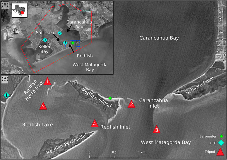
FIGURE 1. Study area map. (A) indicates the study area outlined in red with the blue box indicating the extent shown in (B).

Carancahua Bay is an ideal location to explore questions about living shorelines and morphologic change, as it is at a tipping point in its geological history. The bay inlet has more than doubled in size over the last 20 years (ten-fold increase since 1872), critical habitat has been lost due to ensuing wave erosion, and the bay will soon cease to exist as a distinct circulatory unit from the adjacent Matagorda Bay. As the mouth widens, the entire bay is increasingly exposed to wave erosion and an altered hydrological, salinity, and biological regime. Its unique role as a nursery and refuge, off-limits to commercial fishing and shrimping, is at great risk. Moreover, the large oyster reef and marsh complex at its mouth, supporting mountain laurel and migratory songbird habitat, recreational anglers, and oyster production, is rapidly eroding.

Additionally, the widening at the Carancahua Bay inlet has enhanced wave erosion and threatens public safety (Tompkins and Tresaugue, 2017). As the bay mouth proceeds to widen, the significant wave fetch across West Matagorda Bay will begin to impact the community of Port Alto. A previous living shoreline was placed at Schicke Point to mitigate erosion by an engineering firm funded by a private landowner (Freese and Nichols, 2019). This action proved to be effective at reducing shoreline erosion and encouraged sediment accumulation behind the barrier. Due to the success of the Schicke Point structure, similar structures were proposed to help mitigate erosion at Carancahua inlet. However, the placement of such a structure is complicated by a breach from West Matagorda Bay into Redfish Lake that formed in the late 1980s. This breach continues to widen and has resulted in a dual inlet mouth of Carancahua. The dual inlet system further complicates the hydrologic processes being measured and modeled.

Historic Trends

We conducted both short-term and long-term shoreline change analyses to examine the evolution of Carancahua Bay. All imagery was obtained from the Texas Natural Resources Information System (TNRIS, 2022), the US Geological Survey EarthExplorer interface (USGS, 2022), or digitized nautical maps (NOAA, 2022a).

For the short-term analysis, the shorelines were digitized by hand using aerial imagery for the dates of 1996 and 2018. The rate of shoreline retreat over this date range was then estimated along the entire shoreline. Because of the multi-directional and non-linear nature of shoreline retreat around the geomorphic features of the landscape, the rate was calculated by converting the line data shapefiles into point data with a 10 m spacing. A nearest neighbor analysis was employed to find the points in the direction with the shortest distance.

The long-term analysis assessed change between 1872 and 2018. An 1872 nautical map was georeferenced to the 2018 imagery, and then digitized. Changes from the 1872 to 2018 shoreline were referenced only qualitatively.

The shoreline change data was further examined using related bathymetric sounding datasets (NOAA, 2022a; NOAA, 2022b) and a bathymetric dataset collected in 2020. Historical soundings from 1872 to 1935 were manually entered into a Geographic Information System (GIS) as point data, then interpolated into raster using a standard Inverse Distance Weighting method. Inlet cross-section comparisons were conducted between the years 1872, 1935, and 2020, respectively.

In-Situ Data Collection

In-situ hydrodynamic and sedimentary datasets were collected for two purposes: 1) to understand the general principles of how this multiple-inlet system works, and 2) serve as validation datasets for modeling purposes.

Five sensor tripods were deployed across Carancahua Bay and West Matagorda Bay (Figure 2; Table 1) to collect hydrodynamic and environmental data. Tripods included conductivity temperature and depth (CTD) sensors (VanEssen CTD), wave sensors [Ocean Sensor Systems Sonic Xbees (XB)], and Acoustic Doppler Current Profilers (ADCP) (Nortek Aquadopp Profilers). The sensors were deployed continuously from 18 February 2020 to 2 June 2020.

FIGURE 2

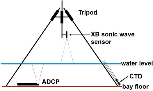
FIGURE 2. The configuration of the sensor tripods and how the XB, ADCP, and CTD sensors were arranged.

TABLE 1

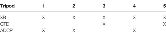
TABLE 1. Sensors deployed on each tripod. See Figure 1 for placement locations.

The XB sensors were used to gather both wave and water level data. An initial sensor deployment on 18 February 2020 was followed up with two more deployments of radio relay stations to improve sensor range and reliability. The sensors were set to record data at 16 Hz for 2 minutes at the start of every hour. Significant wave height (H_s) was extracted from the XB wave data using the zero-up-crossing method over 120 s data segments to determine individual waves before averaging over the largest third of these waves. Tidal currents were simultaneously monitored passing through the Carancahua inlet, the southern inlet of Redfish Lake, and the connection between Carancahua and Redfish Lake, thus a total of three ADCPs were deployed at once (Table 2). ADCP1 was deployed in an upward-looking configuration used to measure water velocity through the water column. The barometrically compensated pressure transducer data from CTD1 was used to reference the water level to ADCP1. Both ADCP2 and ADCP4 were deployed horizontally, or side-looking, allowing them to gaze across the mouths of their respective channels and better sample a wider range of flow behavior. The side looking ADCP’s were mounted on steel frames which positioned the sensor head approximately 45 cm from the bay bottom. The upward-looking ADCP was deployed on a steel frame that set into the soft bay bottom, and positioned so that the bottom of the ADCP casing just touched the bay bottom. All ADCPs were set to sample at 1 Hz for 120 s, at the beginning of every hour.

TABLE 2

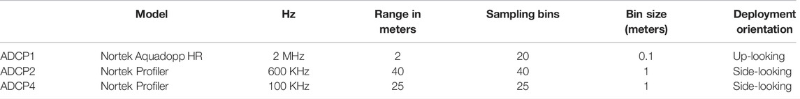
TABLE 2. ADCP configuration.

Sediment grab samples were collected from the upper 5 cm of bed sediment for sensor stands one through 5. Each sample was weighed in a dish of known volume, dried in an oven at 65°C, and reweighed in its dry condition to obtain a measure of bulk density (g/cm³). Each sample was then sieved by using sieves ranging from 2 mm to 15.6 µm (from gravel granules to fine silt and finer). Each subset of sieved particles was weighed and standardized by the total weight of the sample. This procedure yielded the percentage of each sample that was of a given grain size. The mean sediment size was then compared to Hjulstrom-Sundborg diagram to determine settling and erosion velocities (Earle, 2019).

Modeling

The flexible mesh for the Delft3D model was created first as a grid of varying density that acts as the foundation on which all calculations are performed (Figure 3). All model input data is either interpolated to, or applied to, this grid.

FIGURE 3

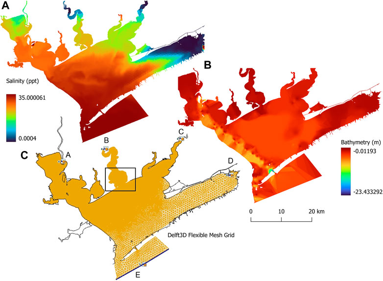
FIGURE 3. (A) The initial salinity input map at the start date, and the integrated bathymetric map. Vertical units for bathymetry are meters (NAVD88). (B) Salinity units are in parts per thousand. Flow model mesh. (C) Input forcing locations are shown for: (A) Lavaca River input boundary, (B) Carancahua Creek input boundary, (C) Tres Palacios River input boundary, (D) Colorado River input boundary, and (E) Gulf of Mexico input boundary. The black box indicates the main area of interest were observation points and barriers were placed.

For inputs to the models, the bathymetry was measured using a custom system composed of a linked depth finder (Matrix 12 by Humminbird) and a survey-grade Global Navigations Satellite System (GNSS) system (Trimble R10). This product was integrated with a coarser Texas Parks and Wildlife Department (TPWD) product, to retain the high resolution for the primary study areas (Figure 3) (TPWD, 2022). The combined bathymetry was then imported into Delft3D and interpolated to the mesh grid.

The inputs to the models included wind direction and velocity, water level, river and creek discharge, and salinity. Wind inputs were sourced from NOAA (NOAA #8773259, Port Lavaca) and applied consistently across the model (NOAA, 2022b). The winds forced the wave generation, using the Hurdle-Stive Fetch/Depth limited model available in Delft3D. Water level data were sourced from NOAA station #8775241 (Port Aransas) and used as forcing condition from 24 January 2020 through 9 July 2020 (boundary E in Figure 3). Salinity was initially set at 35 ppt at the Gulf of Mexico input location. Salinity for all freshwater inflows was set to 0 ppt. River and creek discharge volumes were gathered from USGS river flow gauges (USGS #08162501 for the Colorado river, #08164000 for the Lavaca River, and #08162600 for Carancahua Creek and Tres Palacios River) (USGS, 2022). In order to properly model salinity, an initial version of the flow model was run (with no structural designs) to properly distribute salinity across the basin (Figure 3). This baseline salinity output was then fed back into subsequent models to act as the starting salinity value for each node of the mesh.

The flow model simulations were run to cover dates from 24 January 2020 to 9 July 2020. Model runs typically completed in approximately 12 h on an Intel I9-10900F 10 core 20 thread CPU.

Several living shoreline designs were tested using the numerical model to meet the overall objective of protecting and enhancing habitat in Carancahua Bay, Redfish Lake, and Salt Lake. Living shoreline performance was assessed based on the structures effects on: significant wave heights, water velocity, salinity, reduction of erosion, and potential for habitat creation.

Eight separate models were run, to include seven unique design alternatives and one baseline scenario. The design alternatives can be grouped into two general categories “enclosed” versus “hybrid” as explained below and presented in Figure 4; Table 3. Unless otherwise noted below, the structures’ vertical height was infinite, they were immovable, and they were modeled as “Thin Dams” in Delft3D. The purpose was to simulate the effects of wall-like structures that extended above the maximum water level, at a 30% engineering design phase.

FIGURE 4

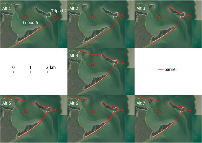
FIGURE 4. Alternatives 1 to 4 are enclosed living shoreline designs and Alternatives 5 to 7 are hybrid living shoreline designs. See text for detailed descriptions of each. Model observation points at tripods 2 and 5 are depicted as red triangles.

TABLE 3

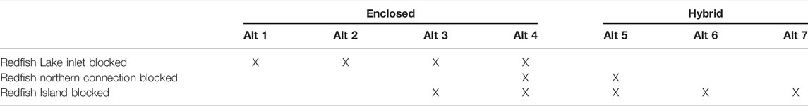
TABLE 3. Major aspects of tested design alternatives.

The enclosed alternatives sought to restore the historic nature of the single inlet at Carancahua Bay inlet by extending a wall-like structure across the inlet of Redfish Lake. The main goal was to shelter Redfish Lake from southerly aspect waves and flow. Considered alternatives included:

Alt 1: “Short”. This alternative tested the general effect of protecting the Redfish Lake area by blocking the Redfish inlet from waves entering from a southerly direction.

Alt 2: “Curved”. This tested effects of curving the structure and more closely hugging the shorelines, while also protecting the Redfish Lake area.

Alt 3: “Extended”. This tested benefits of extending the structure around Redfish Island.

Alt 4: “Full”. This alternative tested benefits of fully blocking all major entrances into Redfish Lake.

The hybrid alternatives sought to retain the dual inlet system at the Carancahua Bay inlet and Redfish Lake by placing perforated structures across the Redfish Lake inlet. The main goal was to shelter Redfish Lake from southerly aspect waves, while also allowing for continued tidal exchange through it.

Alt 5: “Full Perforated”. This alternative tested benefits of protecting Redfish Lake from waves using a perforated structure, through which tidal currents could flow.

Alt 6: “Full Perforated with North Open”. This alternative tested benefits of a perforated structure, while the northern entrance to Redfish Lake remained open.

Alt 7: “Full V-Notch with North Open”. This alternative tested benefits of a V-shaped structure across Redfish Lake inlet, while the northern entrance to Redfish Lake remained open. The structure was emergent 100% of the time in front of Redfish Peninsula and Redfish Island, but partially submerged across the Redfish Lake inlet, grading down in a V-shape to the center of the inlet. The minimum height in the center was 1 m above the bathymetric depth.

Results

Historic Trends

Shoreline retreat between 1996 and 2018 averaged 27 m (median of 15 m) in Carancahua Bay, with a maximum of 293 m and a standard deviation of 37 m. On average, Carancahua Bay shorelines retreated at a rate of 1.22 m/yr. However, large stretches of the southern portion of the bay exceeded this erosion rate. Much of Redfish Peninsula averaged 7 m/yr (Figure 5).

FIGURE 5

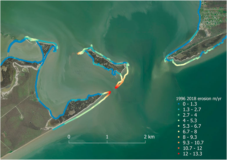
FIGURE 5. Shoreline retreat rates in the southern portion of Carancahua Bay.

From 1872 to 2018, there visually appeared to be a significant amount of change to Redfish Lake, Salt Lake, and at the Carancahua Bay inlet. Most notably, Redfish Lake was fully breached and created a southern entrance and the Redfish Peninsula shoreline retreated northward. The width of the Carancahua inlet grew from 160 m to 2,025 m (Figure 6). In textual notes from a related 1935 survey, the surveyor remarked that there had been significant changes in this area from the 1800s to the 1930s (from 160 to 610 m, respectively; NOAA, 2022b). A clear relationship was found between the width and relative sea level rise (0.0065 m/yr from NOAA #8771450) over this time period (Figure 7). The average widening rate was 12 m/yr.

FIGURE 6

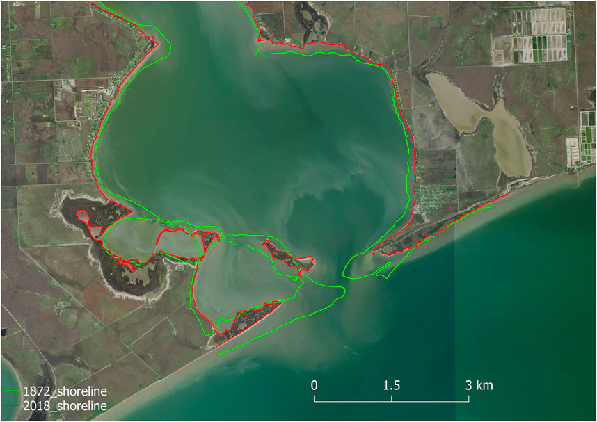
FIGURE 6. Shoreline change from 1872 to 2018.

FIGURE 7

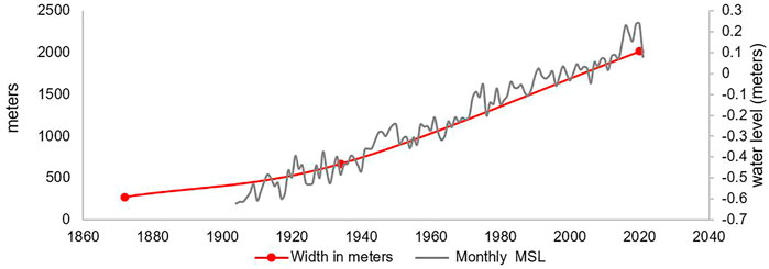
FIGURE 7. The width of the Carancahua Bay inlet and relative water level change over time.

Extrapolating the historical rate at which the bay mouth widened using data points from 1872, 1935, and 2020, the Carancahua inlet will erode all the way to its upland banks by 2082. This calculation used the historical relative sea level rise rate since 1904 (0.0065 m/yr), which differs from the future rate used by the model (0.0076 m/yr). The difference between these two rates is only 17% (as this area had high relative sea level change in the past due to hydrocarbon extraction-induced subsidence, which has since slowed; counter to that, future eustatic change is expected to accelerate; generally, the two offset, albeit with this 17% future increase).

Historically, the Carancahua inlet was narrower, but also considerably deeper, than it is today (Figure 8). Initially it was hypothesized that the inlet changes were the product of increased flow velocities. After calculation of volumetric change over the three dates using the bathymetry and the historical relative sea level rise rate, it was found that the actual volume change could not explain the magnitude of the increase in cross-sectional opening. Additional support for the rejection of this hypothesis is that the mouth shallowed—if the disequilibrium was caused by the volume of tidal pumping alone, one would expect the depth to also increase or at least remain the same.

FIGURE 8

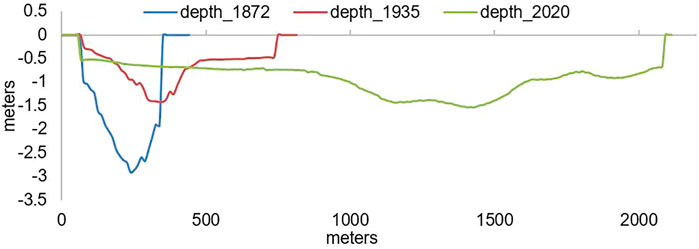
FIGURE 8. Cross-section of the Carancahua Bay inlet over time (NE-SW direction).

In-Situ Data Collection

The in-situ data showed that waves were similar at both the Redfish and Carancahua inlets during southerly winds (∼0.3 m for gauges XB2 and XB4) wile gauges XB1 and XB5 showed lower wave heights at ∼0.2 m. However, during northerly winds, gauge XB1 and XB2 showed similar wave heights at 0.3 m while XB4 was more sheltered from the waves (Figure 9).

FIGURE 9

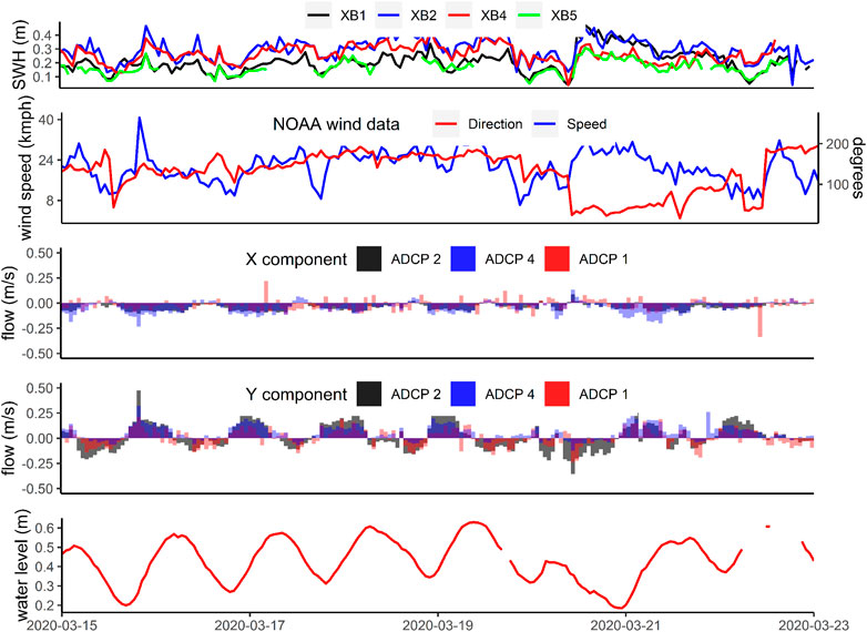
FIGURE 9. Significant wave heights (H₂) at XB1, XB2, XB4, and XB5; NOAA wind speed and direction; ADCP1 (upward-looking, depth averaged), ADCP2 (side-looking, averaged over 20 m across bins 10–20), ADCP4 (side-looking but different model, averaged over 2 m across bins 10–20) flow direction and velocity in X and Y components; and CTD1 water level. Subplot C and D are the Cartesian coordinate components of flow with the X component corresponding to east/west flow. Positive values in subplot C indicate flow towards the east while positive values for subplot D indicate flow to the north.

The ADCP data showed average flow velocities were 0.03 m/s faster through Carancahua inlet and 0.007 m/s slower through Redfish Lake inlet than through the northern connection of Redfish Lake with Carancahua (Figure 9). We also found that Redfish Lake inlet (ADCP4) experienced velocities 0.06 m/s greater during the flood tide than the ebb tide. This is likely the result of the unique behavior of the dual inlet system of Carancahua Bay and Redfish Lake. Water often flowed out of Carancahua inlet (ADCP2) and into Redfish Lake during ebb tides, and the flow velocity was stronger going into Redfish (ADCP4) than coming out (Figure 10). A temporal shift was also seen with ADCP4 where northern flows started before and extended later than the northern flows through Carancahua inlet. This resulted in a circular flow south out of Carancahua and north into Redfish (Figure 10).

FIGURE 10

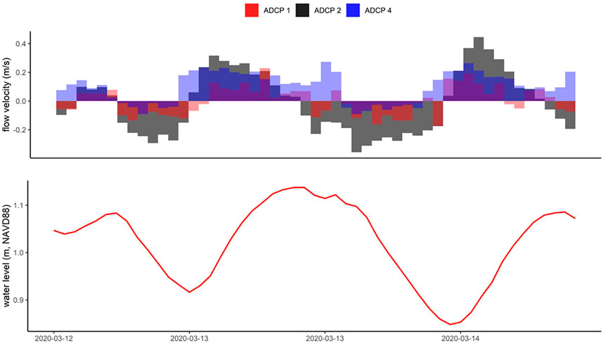
FIGURE 10. Temporal shifts in the water flow direction at the Redfish Lake inlet (ADCP4) are both delayed and lag behind those at the Carancahua inlet (ADCP2). For several hours of the record, they flow in opposite directions.

The sedimentary data showed a mean erosion velocity of the subtidal bottom sediments [0.35 m/s, mean grain size (mm) of 0.20] and along the unconsolidated shorelines [0.40 m/s mean grain size (mm) of 0.08] are near the peak velocities seen during the tidal cycle. Under the current wave and flow conditions at the Carancahua inlet, the mean erosion velocity of 0.35 m/s was exceeded 5.76% of the time.

Modeling

To validate the models, wave, flow velocity, water level, and salinity predictions were compared against observations. The focus was on validating the model performance against the baseline in-situ data across 24 January 2020 to 9 July 2020. Visual comparisons of the results at finer time scales, for example from 15 March 2020 to 23 March 2020 indicated acceptable model agreement with the field data (Figure 11).

FIGURE 11

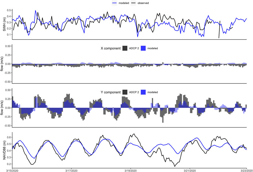
FIGURE 11. Comparison of measured and modeled hydrodynamics at Carancahua inlet.

Due to the tidal boundary input data not matching the location of the modeled boundary, the baseline model was tuned further using an iterative process. The tidal amplitude and timing at the Gulf of Mexico boundary was adjusted to reduce the mean error between the modeled and observed values to levels below 10% (5.22% measured deviation, mean error of 0.022 m). Mean water levels were the same between the model and observed data with the model overpredicting mean significant wave height by 0.03 m and underpredicting mean flow velocities by 0.003 m/s. The largest discrepancies were found for maximum flow velocities in the north-south direction, with the model under-predicting values by 43%. At the Carancahua inlet (Tripod #2 location), the average velocities were 0.089 m/s slower in the modeled product than the ADCP data in the Y direction and 0.041 m/s slower in the X direction (Figure 11). The apparent differences were likely due to an incomplete representation of the intersection of Redfish Lake, Carancahua Bay, and Matagorda Bay in the Delft3D model resulting from the need for higher resolution bathymetry.

Compared to the baseline scenario, no alternatives reduced the wave energy impacting Carancahua Bay or Redfish Lake by more than 25%, in immediate terms for the year 2020 (Table 4).

TABLE 4

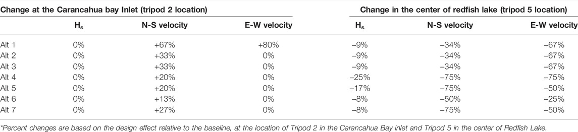
TABLE 4. The effect of various design alternatives on existing waves and flow velocities.

Secondly, structures that blocked tidal flows at Redfish Lake inlet proportionally increased flows through the other side of this dual inlet. For example, Alt 2: “Curved” and Alt 3: “Extended” increased the average north-south flow velocities at the Carancahua inlet by 33% (Table 4).

Hybrid, perforated structures also increased velocities in the Carancahua inlet, but to a lesser extent on average (Table 4), for example Alt five increased them in the north-south direction by 20%. This partial blocking was deemed more acceptable in terms of quantity of time that flow exceeded the erosion threshold.

Thirdly, alternatives that avoided blocking the northern entrance to Redfish Lake relieved a portion of the energy created when partially blocking the inlet to Redfish Lake. For example, Alt six increased north-south velocities in the Carancahua inlet by only 13%, while also reducing them in Redfish Lake by −50%.

Discussion

The shoreline change analysis and field datasets showed that flows through the Redfish Lake inlet were primarily generated by wave action, while those through the Carancahua inlet were primarily tidal, and this behavior is related to both tidal flow direction and wind-driven wave direction (Figures 9, 10). It is likely that relative sea level rise promoted the conditions under which the waves accessed and excavated the sediments on the Redfish Peninsula; the perforation of the Peninsula was likely the direct result of wave erosion as opposed to tidal current scouring (Schwartz, 1967). Once the sediments were eroded by the waves, tidal currents then moved them out into a submerged ebb tidal shoal in West Matagorda Bay as well as entrained them into the littoral drift moving to the southwest of the Redfish Peninsula. Accordingly, it is likely the case that the widening and shallowing over time of the inlet at the Carancahua inlet is indirectly related to relative sea level rise, as waves gained access to higher sections of shoreline. These waves then loosened the sediments and tidal flow exported them.

Generally, a wall-like structure across the Redfish Lake inlet or Carancahua Bay will not greatly reduce wave heights within these basins in 2020. The fetch length within the Redfish Lake basin is sufficient to re-build the maximum wave heights that are allowable given its depths. Thus, adding a barrier to its mouth will not materially change the ability of waves larger than these heights to make it into the basin, at least in the present day under existing conditions. The same effects can be seen for Carancahua Bay (Table 4). However, as shown by the shoreline change analysis, waves in these basins will completely erode the Redfish Peninsula and Redfish Island by 2082. Although the results are not shown here, further modeling work corroborated this finding and showed that waves should be expected to increase three-fold between 2020 and the year 2100 in Redfish Lake and Carancahua Bay.

While many other studies examine much larger engineered structures, it has been well demonstrated that placement of hardened structures can cause unintended erosion (Toso et al., 2019). Structure placement will alter flow velocities, and closing the Redfish Lake inlet will result in a proportional increase in flow velocities in Carancahua inlet. As velocities are already exceeding the mean erosion threshold approximately 5% of the time at Carancahua inlet, any increase in velocity will further accelerate sediment transport. This situation presents challenges with any ‘enclosed’ design as increased scour at Carancahua is unavoidable. Conversely the ‘hybrid’ structures allowed for some flow relief while still providing protection long term (Khojasteh et al., 2020). The hybrid structures showed only an average of 20% increase in velocity at Carancahua inlet compared to the 38% increase with the enclosed designs. The hybrid designs offer a greater margin of safety especially when considering the added erosive energy tropical events could exert on the bay system. Moreover, our validation datasets showed that the Delft3D models underpredicted the velocities that were observed. Thus, it is likely that real-world velocities will exceed our predictions. The “enclosed” designs have the potential to cause erosion that is beyond the predictive ability covered by the current research. For this reason, the safest decision is for coastal managers to use a “hybrid” design alternative. This narrows down the possible structures to Alternatives 5–7. All three designs reduce wave heights and water velocities in the center of Redfish Lake, however, Alternatives 5 and 7 increase water velocities within Carancahua inlet by 20% or more while Alternative 6 only increased velocities 13%. A major goal was to not increase erosive velocities, therefore Alternative 6 was selected for further analysis.

Conclusion

Without intervention the Carancahua inlet will erode completely to the edge of the uplands to the west of the Redfish Peninsula by 2082. Carancahua Bay will fully merge with West Matagorda Bay, with detrimental consequences for wave generation, shoreline erosion, and impacts to properties and aquatic habitats.

A living shoreline structural design that allows the maintenance of the existing dual inlet system will help maintain acceptable flow velocities through the Carancahua inlet, while still creating a barrier to wave energy and reducing sediment export velocities out of Redfish Lake. For this reason, we contend that Alt 6: “Full Perforated with North Open” best mitigates wave heights, reduces erosion, and reduces risks. The selected Alt 6 design will need to undergo further analysis by a modeling specialist before implementation. The future work should include the addition of morphology in the evaluation of Alt 6 in addition to the utilization of a SWAN model to drive the wave calculations. However, this study shows the utility of Delft3D in helping to design living shorelines, particularly within the context of a complex dual inlet system that is adjusting to sea level rise.

Data Availability Statement

The raw data supporting the conclusion of this article will be made available by the authors, without undue reservation.

Author Contributions

RF acquired project funding in conjunction with JF with TH aiding in experimental design of and sensor selection. TH handled computer computation analysis with guidance of both RF and JF. TH conceived and created the figures and written material. Both JF and RF assisted with revisions and paper scope.

Funding

This work was supported in part by funds provided by the Texas General Land Office (20-106-000-C051) to TH, RF, and JF; US Fish and Wildlife Service to RF (FWS/R2/ES/F17AC00461); National Science Foundation (1756477) to RF; National Institute of Food and Agriculture (91380) to RF.

Conflict of Interest

The authors declare that the research was conducted in the absence of any commercial or financial relationships that could be construed as a potential conflict of interest.

The handling editor RS declared a past co-authorship with the author RF.

Publisher’s Note

All claims expressed in this article are solely those of the authors and do not necessarily represent those of their affiliated organizations, or those of the publisher, the editors and the reviewers. Any product that may be evaluated in this article, or claim that may be made by its manufacturer, is not guaranteed or endorsed by the publisher.

Acknowledgments

We would like to thank the TAMU Coastal Ecology and Management Lab graduate students (Rachel Innocenti and Mathew “Jake” Madewell) for their assistance in data collection and processing. We also appreciate the help provided by Bill Balboa from the Matagorda Bay Foundation and Dave Buzan from Freese and Nichols.

References

Bennett, W. G., van Veelen, T. J., Fairchild, T. P., Griffin, J. N., and Karunarathna, H. (2020). Computational Modelling of the Impacts of Saltmarsh Management Interventions on Hydrodynamics of a Small Macro-Tidal Estuary. J. Mar. Sci. Eng. 8, 373. doi:10.3390/jmse8050373

CrossRef Full Text | Google Scholar

Cooper, J. A. G., and McKenna, J. (2008). Social Justice in Coastal Erosion Management: The Temporal and Spatial Dimensions. Geoforum 39, 294–306. doi:10.1016/j.geoforum.2007.06.007

CrossRef Full Text | Google Scholar

Delft3D [computer software] (2021). Deltares. Retrieved from https://oss.deltares.nl. (Accessed May 13, 2021).

Google Scholar

Earle, S. (2019). Physical Geology. 2nd Edition. Victoria, BC: BCcampus.

Google Scholar

Elias, E. P. L., Walstra, D. J. R., Roelvink, J. A., and Stive, M. J. F. (2000). “Hydrodynamic Validation of Delft3D with Field Measurements at Egmond,” in 27th International Conference on Coastal Engineering. Sidney Australia, July 16-21, 2000.

Google Scholar

Freese and Nichols (2019). A Living Shoreline. Available at: https://www.freese.com/a-living-shoreline/(Accessed 17 5, 2022).

Google Scholar

Horstman, E., Dohmne-Janssen, M., and Hulscher, S. (2013). “Modeling Tidal Dynamics in a Mangrove Creek Catchment in Delft3D,” in Coastal Dynamics. Editors P. Bonneton, and T. Garlan (Bordeaux: Bordeaux University), 833–844.

Google Scholar

Hoyt, J. H. (1967). Barrier Island Formation. Geol. Soc. Am. Bull. 78, 1125–1136. doi:10.1130/0016-7606(1967)78[1125:bif]2.0.co;2

CrossRef Full Text | Google Scholar

Huff, T. P., and Feagin, R. A. (2017). Hydrological Barrier as a Cause of Salt Marsh Loss. J. Coast. Res. 77, 88–96. doi:10.2112/si77-009.1

CrossRef Full Text | Google Scholar

Khojasteh, D., Hottinger, S., Felder, S., De Cesare, G., Heimhuber, V., Hanslow, D. J., et al. (2020). Estuarine Tidal Response to Sea Level Rise: The Significance of Entrance Restriction. Estuar. Coast. Shelf Sci. 244, 106941. doi:10.1016/j.ecss.2020.106941

CrossRef Full Text | Google Scholar

Miller, J. K., Rella, A., Williams, A., and Sproule, E. (2016). Living Shorelines Engineering Guidelines. Stevens Institute of Technology. Available at: http://stewardshipcentrebc.ca/PDF_docs/GS_LocGov/BkgrdResourcesReports/living-shorelines-engineering-guidelines.pdf.

Google Scholar

Morris, J. T., Sundareshwar, P. V., Neitch, C. T., Kjerfve, B., and Cahoon, D. R. (2002). Response of Coastal Wetlands to Rising Sea Level. Ecology 83 (10), 2869–2877. doi:10.1890/0012-9658(2002)083[2869:ROCWTR]2.0.CO;2

CrossRef Full Text | Google Scholar

Muñoz, D. F., Yin, D., Bakhtyar, R., Moftakhari, H., Xue, Z., Mandli, K., et al. (2022). Inter‐Model Comparison of Delft3D‐FM and 2D HEC‐RAS for Total Water Level Prediction in Coastal to Inland Transition Zones. J Am. Water Resour. Assoc. 58, 34–49. doi:10.1111/1752-1688.12952

CrossRef Full Text | Google Scholar

NOAA (2022a). Coast Chart #107 Matagorda Bay Texas. Historical Map and Chart Collection. Available at: https://historicalcharts.noaa.gov/image=AR22-00-1869 (Accessed 0218, 2022).

Google Scholar

NOAA (2022b). NOAA Tides and Currents. Available at: https://tidesandcurrents.noaa.gov (Accessed 0216, 2022).

Google Scholar

Passeri, D. L., Hagen, S. C., Medeiros, S. C., and Bilskie, M. V. (2015). Impacts of Historic Morphology and Sea Level Rise on Tidal Hydrodynamics in a Microtidal Estuary (Grand Bay, Mississippi). Cont. Shelf Res. 111, 150–158. doi:10.1016/j.csr.2015.08.001

CrossRef Full Text | Google Scholar

Schwartz, M. L. (1967). The Bruun Theory of Sea-Level Rise as a Cause of Shore Erosion. J. Geol. 75, 76–92. doi:10.1086/627232

CrossRef Full Text | Google Scholar

Smith, C. S., Rudd, M. E., Gittman, R. K., Melvin, E. C., Patterson, V. S., Renzi, J. J., et al. (2020). Coming to Terms with Living Shorelines: A Scoping Review of Novel Restoration Strategies for Shoreline Protection. Front. Mar. Sci. 7, 434. doi:10.3389/fmars.2020.00434

CrossRef Full Text | Google Scholar

Smith, K. (2006). "Management, Policy, Science, and Engineering of Nonstructural Erosion Control in Chesapeake Bay: Proceeding of the 2006 Living Shoreline Summit," in Integrating Habitat and Shoreline Dynamics Into Living Shoreline Applications. Williamsburg, Virginia: Chesapeake Bay National Estuarine Research Reserve

Google Scholar

Sutherland, j., Walstra, D. J. R., Chester, T. J., Van Rijn, L. C., and Southgate, H. N. (2004). Evaluation of Coastal Area Modelling Systems at an Estuary Mouth. Coast. Eng. 51 (2), 119–142. doi:10.1016/j.coastaleng.2003.12.003

CrossRef Full Text | Google Scholar

TNRIS (2022). Texas Natural Resources Information System. Available at: https://tnris.org (Accessed 22 3, 2022).

Google Scholar

Tompkins, S., and Tresaugue, M. (2017). Death of Three Hunters a Cautionary Tale. Available at: https://www.houstonchronicle.com/sports/outdoors/article/Death-of-three-hunters-a-cautionary-tale-10851671.php (Accessed 17 5, 2022).

Google Scholar

Toso, C., Madricardo, F., Molinaroli, E., Fogarin, S., Kruss, A., Petrizzo, A., et al. (2019). Tidal Inlet Seafloor Changes Induced by Recently Built Hard Structures. PLoS One 14, e0223240. doi:10.1371/journal.pone.0223240

PubMed Abstract | CrossRef Full Text | Google Scholar

TPWD (2022). Texas Parks and Wildlife Geographic Information Systems. Available at: https://tpwd.texas.gov/gis/(Accessed 22 3, 2022).

Google Scholar

USGS (2022). United States Geological Survey. Available at: https://waterdata.usgs.gov/nwis/rt (Accessed 22 3, 2022).

Google Scholar

Vona, I., Palinkas, C. M., and Nardin, W. (2021). Sediment Exchange between the Created Saltmarshes of Living Shorelines and Adjacent Submersed Aquatic Vegetation in the Chesapeake Bay. Front. Mar. Sci. 8, 727080. doi:10.3389/fmars.2021.727080

CrossRef Full Text | Google Scholar

Weaver, R. J., Stehno, A., Bonanno, N., Sager, A., Kenny, A., Zehnder, J. A., et al. (2017). Scale Model Design of Oyster Reef Structures as Part of a Showcase Living Shoreline Project. Shore Beach 85, 41–54.

Google Scholar

White, W. A., Tremblay, T. A., Waldinger, R. L., and Calnan, T. R. (2006). Status and Trends of Wetland and Aquatic Habitats on Texas Barrier Islands, Coastal Bend. Austin, Texas: The University of Texas at Austin, Bureau of Economic Geology Final Report Prepared for Texas General Land Office and National Oceanic and Atmospheric Administration Under Contract 05-041, 65.

Google Scholar

Williams, A. T., Rangel-Buitrago, N., Pranzini, E., and Anfuso, G. (2018). The Management of Coastal Erosion. Ocean Coast. Manag. 156, 4–20. doi:10.1016/j.ocecoaman.2017.03.022

CrossRef Full Text | Google Scholar