Can apparent resting state connectivity arise from systemic fluctuations?

Introduction

The use of resting state functional MRI (rsfMRI) to study baseline brain activation in the absence of external stimuli has increased dramatically in recent years (Biswal et al., 1995; Greicius et al., 2003; Fox et al., 2005; Damoiseaux et al., 2006). Resting state network (RSN) analysis is based on the premise that information is exchanged between functionally related brain regions continuously, even during rest, leading to correlated neuronal activations among these regions in resting state. These correlated neuronal activations in turn lead to coherent spontaneous low frequency (~0.1 Hz) fluctuations in blood oxygen level dependent (BOLD) signals through neurovascular coupling.

Implicit in these analyses are a number of assumptions that are not frequently articulated. The first is that the hemodynamic response to spontaneous neuronal activations is the main source of spatially correlated low frequency oscillations observed in the BOLD signal. The second is that within each RSN, synchronized neuronal activations lead to high temporal correlations between the BOLD signals from these functionally related regions. Finally, it is generally assumed that the particular pattern of coupled spontaneous neuronal activations is unique to each RSN, leading to different timecourses for each of the networks. Therefore, we are able to identify different RSNs using correlation analysis, in which we search for the regions that share the same low frequency BOLD signals, either using a seed region placed in an area of interest (Biswal et al., 1995; Hampson et al., 2002) (i.e., seed analysis), or a data-driven independent component analysis (ICA) (Calhoun et al., 2001; Beckmann et al., 2005), where independent spatiotemporal RSNs can be derived simultaneously without a predetermined regressor.

However, as we know, the BOLD signal is not a direct measurement of neuronal activation, but rather a measurement of changes in blood flow, oxygenation, and volume (Obrig et al., 2000; Wise et al., 2004; Birn et al., 2006; Tong and Frederick, 2012). While these changes can be, and are, caused by neuronal activation through neurovascular coupling, they can also arise from any other physiological processes that affect blood oxygenation or volume. In our recent resting state studies, we have found that a significant portion of the slow oscillations (~0.1 Hz) observed in BOLD fMRI is closely associated with the propagation of systemic low frequency oscillations (sLFOs) through the vasculature (Tong and Frederick, 2010, 2014). The reason these sLFOs are called “systemic” is that the same signals found propagating through the brain, are found in the periphery (e.g., fingertips and toes) as well, when using simultaneous near infrared spectroscopy (NIRS) recordings (Tong and Frederick, 2012; Tong et al., 2013). Although the origins and functions of these sLFOs are not known (Sassaroli et al., 2012), it is clear that temporally shifted versions of this signal are widely present in the BOLD signal of the majority of the voxels in the brain. They seem to travel with the blood and reach different voxels at different time delays determined by the path blood takes through the cerebral vasculature.

Brain regions with similar vascular time delays will have high temporal correlations, since the sLFOs will arrive in these regions at the same time. Because of the high symmetry in the cerebral vasculature, these correlated regions will tend to be symmetric. Blood takes ~6–9 s to travel from the carotid arteries to the jugular veins through which it leaves the head (Crandell et al., 1973; Schreiber et al., 2002; Tong and Frederick, 2010), so for any time lag within this range, there will be a pattern of spatial voxels sharing a timecourse at that delay time. This is very different from patterns derived from spontaneous neuronal activities, in which high correlations between regions mean that the regions share a signal derived from the unique neuronal fluctuations for each network. However, correlation-based RSN analyses might not be able to differentiate the sLFOs related correlations from neuronal ones.

In this study, we examine to what extent apparent connectivity may arise from these non-neuronal sLFOs alone, using commonly used RSN analyses, such as ICA and seed analysis. We focus primarily on ICA analysis here, as we feel that ICA's sensitivity toward temporal shifts in the BOLD signals, and how that sensitivity affects these analyses, is not widely known.

To determine whether time shifted systemic signals can result in apparent RSNs, we must answer three questions.

(1) What does ICA do when presented with image data consisting of multiple regions with the same timecourse, differing only in the temporal shift of the timecourse? In other words, could ICA derive multiple different networks from moving sLFOs alone? To answer this question, we applied ICA on synthetic BOLD data consisting of regions with the same timecourse over the range of time delays (−2 to +2 s, about the range of blood arrival times observed in the majority of the brain in vivo), to see if separate networks were generated.

(2) What is the distribution (amplitude and delay) of sLFO signals seen in real subjects' task free data? In other words, can we quantify the parameters of the sLFO signals in each brain voxel? We have addressed this question in our previous work (Tong and Frederick, 2014) and will discuss it briefly in the methods. In short, we are able to accurately calculate the arrival time and amplitude of sLFOs at each relevant voxels in resting state data using two different methods.

(3) What kind of networks would be generated from these moving sLFOs alone using common methods, in the absence of any neuronal signals? Are these networks of sLFOs similar to the well-known RSNs? To assess this problem, we performed a group analyses (seed based and ICA) on synthetic BOLD data (where each voxel has an identical timecourse, delayed by the voxel-specific temporal delays of the sLFOs calculated from the real data). These synthetic data only reflect the subject-specific propagating information of these sLFOs in the brain, not neuronal signals. The resulting “networks” were compared with well-known RSN templates as well as RSNs derived from the real resting state BOLD data of the same group of subjects.

Materials and Methods

Protocol

fMRI resting state studies were conducted in 11 healthy participants (6 M, 5 F, average age ± SD, 31.3 ± 11.7 years). In the resting state studies, participants were asked to lie quietly in the scanner with their eyes open and view a gray screen with a fixation point in the center. The resting state scans lasted 360 s for 11 participants. The Institutional Review Board at McLean Hospital approved the protocol and informed consent from was signed by every participant before the experiment.

All MR data were acquired on a Siemens TIM Trio 3T scanner (Siemens Medical Systems, Malvern, PA) using a 32-channel phased array head matrix coil. After acquiring a high resolution localizer image, (MPRAGE, TR/TI/TE = 2530/1100/3.31, 256 × 256 × 128 voxels over a 256 × 256 × 170 mm sagittal slab, GRAPPA factor of 2), multiband EPI (University of Minnesota sequence cmrr_mbep2d_bold R008) (Moeller et al., 2010; Xu et al., 2013) data was obtained with the following parameters: (TR/TE = 400/30 ms, flip angle 43°, matrix = 64 × 64 on a 220 × 220 mm² FOV, multiband factor = 6, 30, 3.0 mm slices with 0.5 mm gap parallel to the AC–PC (anterior commissure–posterior commissure) line extending down from the top of the brain. Concurrently, a MRI-compatible optical NIRS probe (1.5 cm separation between collection and illumination fibers) was placed over the tip of the left middle finger. NIRS data was recorded continuously before, during and after the resting state fMRI acquisition with an ISS Imagent (ISS, Inc., Champaign, IL) at 690 and 830 nm with 12.5–25 Hz acquisition rate.

Analytical Method

For each participant, the standard fMRI preprocessing steps, including brain extraction, motion correction, slice-time correction, smoothing (5 mm) were applied to the original BOLD signals (using FEAT v6.00 of FSL 5.0) (Jenkinson et al., 2012). We then applied a Fourier domain bandpass filter (0.01–0.2 Hz) in MATLAB (The Mathworks, Natick, MA) on all the resulting data to remove the high frequency physiological signals of respiration and cardiac pulsation from the BOLD data (which was possible due to the ultrafast fMRI acquisition).

Simulations – ICA

Since the signal power of the resting state BOLD data is mainly in the low frequency range, we used a combination of multiple sinusoid waves of different low frequencies (0.01–0.2 Hz) to simulate a basic BOLD fMRI timecourse (as shown in Equation 1). Moreover, we generated synthetic propagating sLFO waves in two symmetrical regions (rectangular) as shown in Figure 1 by progressively delaying this timecourse in the y direction. The propagating wave started at the anterior portion of these two areas and gradually “moved” toward the posterior (as indicated by the arrows). To reflect this, we used the BOLD signal (as in Equation 1) with gradually changing Δt (BOLD(t + Δt)) to simulate the BOLD signals in these areas [Δt gradually changed from −2 to +2 s as the wave moved from anterior to posterior within the areas (see Figure 1)]. The 4 s range of propagation delays was selected based on the mean transit time of the cerebral blood flow in the brain seen in previous studies (Crandell et al., 1973; Schreiber et al., 2002). The TR in the synthetic dataset is 2 s and a total of 195 volumes were calculated. To match properties of real fMRI data, the synthetic BOLD signal of each voxel had a mean of 10⁴ and a standard deviation of 4% of the mean. White noise with a standard deviation of 1% of the mean was added to each voxel to simulate scanner noise.

$\begin{array}{cc}\begin{array}{l}BOLD(t)=0.8\times \text{sin }\left(0.01·2\pi ·t\right)+1\times \text{sin }\left(0.05·2\pi ·t\right)\hfill \\ +0.3\times \text{sin }\left(0.1·2\pi ·t\right)+0.2\times \text{sin }\left(0.2·2\pi ·t\right)\hfill \\ +0.2\times \epsilon (t);\hfill \end{array}& (1)\end{array}$

ε(t) is the white random noise generated by a MATLAB function (random).

FIGURE 1

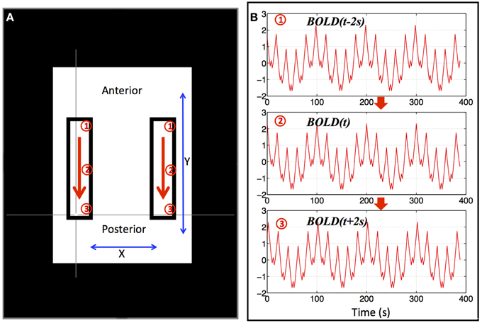
Figure 1. Synthetic data for a single “subject.” Two identical blocks were selected, as shown in (A), in which, artificial traveling waves (as shown in B) were used to replace the original BOLD signals. The red arrows indicate the direction of the traveling wave and synthetic data from three positions marked by circled numbers (1–3) were shown in (B). The remaining BOLD signal was also replaced by an identical synthetic data as (2) in (B).

We applied Melodic ICA (Multivariate Exploratory Linear Optimized Decomposition into Independent Components (Melodic 3.10) (Beckmann and Smith, 2004; Beckmann et al., 2005) from FSL (Smith et al., 2004; Jenkinson et al., 2012) on this single subject's synthetic data with spatial smoothing (5 mm), variance normalization and a fixed dimensionality of 10 components.

Group ICA on All Subjects

Resting state analysis – Group ICA on real data

We performed a group MELODIC ICA analysis on all 11 participants' real resting state data with the following setups: spatial smoothing (5 mm), variance-normalize timecourses, multi-session temporal concatenation. The dimensionality in MELODIC was set to 30, a number routinely used for ICA studies (Beckmann and Smith, 2004). The final results were all registered to the MNI152 2 mm³ standard space template (Montreal Neurological Institute, Montreal, QC, Canada).

Resting state analysis – Group ICA on synthetic data

The analysis of the previous section was repeated on synthetic datasets with no neuronal information. To generate the synthetic data, we first calculated the 3D sLFO delay map from each subject's own resting state data. The delay map (3D image) reflects the subject-specific propagation of the sLFOs throughout the brain. The value of the voxel in a delay map marks the relative arrival time of the sLFOs at this voxel. For instance, a value of 2.0 means that the sLFOs arrived at this voxel 2 s later than the time arrival time at a reference voxel. We then generated synthetic systemic BOLD data (using the timecourse shown in Equation 1) for each voxel, where the same timecourse, representing the systemic signal, is used in every voxel; in each voxel the temporal shift of this timecourse is determined by the delay value for that voxel and scaled to the local BOLD signal intensity. For instance, the synthetic timecourse will be shifted by 2 s in the voxel, for which the delay value is 2 and then the whole timecourse will be rescaled to the intensity of the original BOLD. NB: the timecourse itself is arbitrary – the only important characteristic is that the signal is bandlimited to the low frequency range (0.01–0.2 Hz). Using sums of sinusoids, filtered white noise, or the subject's actual fingertip NIRS signal yields the same results.

In order to ensure that the delay map estimation was not in some way contaminated by neuronal signals, the delay maps were generated twice using two independent procedures. The first procedure used was a data-driven recursive method. The details of the method can be found in our previous publication (Tong and Frederick, 2014). In short, the data-driven method employs a recursive procedure to extract sLFOs from the BOLD signals of each subject. The procedure starts with seed selection. Since we believe these sLFOs are related to the blood signal, the seed is chosen from a blood vessel voxel (e.g., in the Superior Sagittal Sinus) to avoid neuronal activation. The timecourse of the seed is extracted and used as a regressor to cross-correlate with all the BOLD signals from the rest of the voxels. Voxels were selected that met the following conditions: (1) the highest correlation is greater than 0.5; (2) the time lag of this highest correlation is 1 (or −1, depending on the direction of the flow we are tracking. Unit:TR).

The averaged timecourse of these voxels becomes the new “seed” regressor and the procedure is repeated. Every new regressor is similar to the previous regressor (high correlation) while being temporally shifted by one TR, representing sLFO signals that have moved in space compared to the voxels detected by the previous regressor (an example of these regressors is depicted in Supplementary Figure 1). This set of regressors is then used to assess the arrival time of sLFOs at relevant voxels statistically by using FSL FEAT (see details in Tong and Frederick, 2014). The temporal delay was derived only from those voxels having significant correlations (z > 6) with one of these regressors. This is critical to guarantee the delay time calculated is from the sLFOs, not from other signals in the BOLD. In the final delay-map, the value in each voxel represents the relative arrival time of these sLFOs at the specific voxel. We synthesized the data using the delay maps for all 11 subjects.

In the second procedure, we used our previously described method (Tong et al., 2011), in which the oxyhemoglobin concentration timecourse measured by NIRS in the periphery is used as a systematic physiological noise regressor. We first converted the raw optical data into the changes in oxy-hemoglobin concentration (Δ[HbO]) and the changes in deoxy-hemoglobin concentration (Δ[Hb]) (Matcher et al., 1994). We extracted the corresponding timecourse of Δ[HbO] (over the time range matching the fMRI scan) and downsampled it to the fMRI TR (0.4 s). The voxel-wise cross correlation with this timecourse was calculated. For each voxel, the temporal shift corresponding to the maximum correlation coefficient (threshold is R = 0.15) is used as the temporal delay of that voxel. Δ[HbO] is used instead of Δ[Hb] because of its significantly higher signal-to-noise ratio (SNR) (Zhang et al., 2010b; Niu et al., 2011) due to it's higher concentration (the oxygen saturation of the blood in the periphery is typically over 95%). After obtaining the delay-map, the synthetic data of 11 subjects was generated using the procedure described above.

Once the synthetic datasets were constructed, group MELODIC analyses with the same parameters used in the previous analysis of real data were performed on each set of synthetic data. The results were compared with a widely used RSN template (Beckmann et al., 2005). For a fair comparison of the results from the real and synthetic data (both were put through the same procedures), we rescaled the synthetic data by the mean and amplitude of the corresponding real BOLD signal, leaving the temporal oscillation the only distinct variable. The scaling effect will not affect the result since the variances have been normalized in the process (i.e., variance–normalize).

Seed Analysis of Real and Synthetic Data (Group)

In addition to the ICA analysis, the real and synthetic data underwent a seed analysis. The default mode network (DMN) was selected due to its robustness. The DMN seed was a 10 mm spherical region of interest in the posterior cingulate cortex (Watanabe et al., 2013) centered at the MNI coordinates 45, 35, and 49. The average timecourse across all voxels within the region of interest were extracted for every individual participant. The resulting timecourses were used as regressors in a subject-specific general linear model (FSL Feat – Lower level analysis) to define the DMN. A second-level mixed-effects analysis (FSL Feat – Higher level analysis) was subsequently run to define the average DMN across all subjects. At the group level, statistics were corrected for multiple comparisons using a cluster threshold of z = 2.3, p < 0.05.

Results

Figure 2 shows the results of an ICA of the synthetic data from a single “subject” where a single arbitrary timecourse is given a time shift proportional to its vertical position within the highlighted box (as shown in Figure 1). Among 10 resulting independent components (IC), five IC patterns related to the artificially moving sLFO waves were identified, including the patterns: (1) associated with large, intermediate, and small sizes (as shown in Figure 2A, Figure 2B, and Figures 2C,D, respectively); (2) associated with different locations inside the highlighted box (as shown in Figures 2A,C,E); (3) associated with uniform (in Figures 2A,B) or scattered distribution as shown in Figure 2E. All the patterns are symmetric.

FIGURE 2

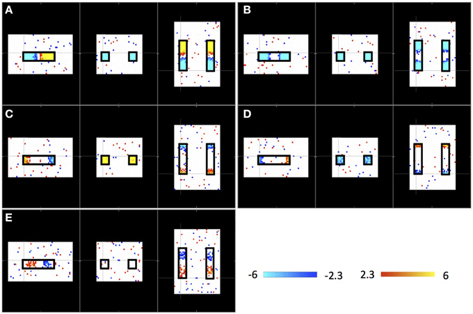
Figure 2. Five ICs (A–E) resulting from ICA on a single “subject.” Each IC pattern is shown in three viewpoints (Sagittal, Coronal, and Axial). The locations of synthetic traveling waves are indicated by the black boxes in all three views. The color bar represents the z-value as result of ICA.

Figure 3 shows an example delay map of one subject derived using the recursive method, together with the temporal delays of three example voxels and their synthetic timecourses. In addition, a similar delay map (of the same subject) derived from the NIRS method is shown as an inset in Figure 3A (upper left). The following observations can be made: First, the variations of the colors in the map indicate that these sLFOs do reach different voxels at different times. The overall systematic color patterns reflect the underlying cerebral blood vasculature. For example, the longer delays (shown as red-yellow in Figure 3) happen at the draining veins (i.e., Superior Sagittal Sinus, straight sinus). Second, the time it takes a wave to propagate through the entire brain is about 7 s, which is consistent with the mean transit time of cerebral blood flow (Crandell et al., 1973). Lastly, the draining system (with clearly identifiable veins) is more prominent in the map than the arteries are. This is because BOLD fMRI is more sensitive to veins than arteries (Menon, 2012). To demonstrate the significance of the BOLD signal correlation with these sLFO regressors, we showed the maximum z-statistic map of the same subject in Figure 4A. The maximum z-value at each voxel reflects the significance of the correlation between the BOLD signal of that voxel and the corresponding recursive regressor. From Figure 4A, we can observe that most of the BOLD signal is significantly correlated with one of these regressors (max z > 6). This significance threshold is more stringent than Bonferroni correction. The most significant z-values (max z > 30) are found in the gray matter as well as large draining veins. Figure 4B shows the corresponding histogram of the maximum z-statistic map, which further demonstrates the significant correlations between sLFOs and BOLD and the wide spatial extent of the sLFOs in the BOLD signals.

FIGURE 3

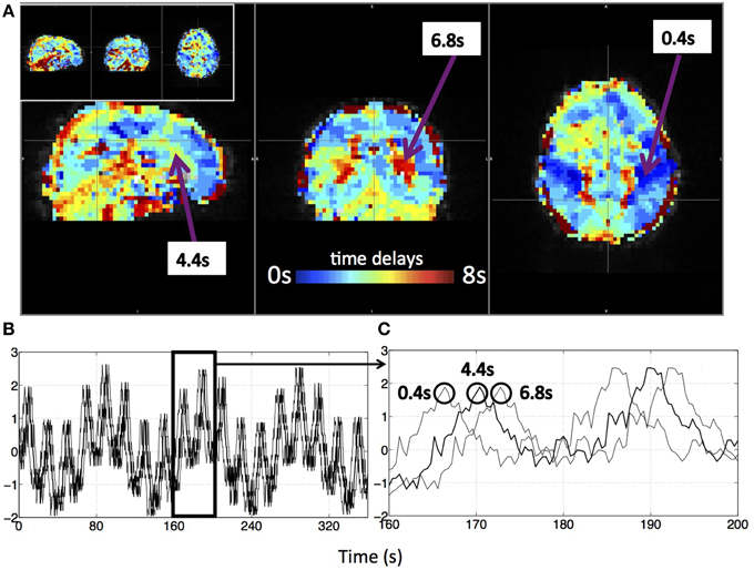
Figure 3. A delay map of the synthetic data of one subject derived with the recursive method (A) and its synthetic BOLD data (B,C). Three example voxels were selected from the delay map with their time delays (A) and the corresponding synthetic temporal traces were shown in (B). (C) The enlarged section of (B) with circles indicating the corresponding voxel of the marked trace. The delay map derived with the NIRS method of the same subject is shown as an inlet in (A).

FIGURE 4

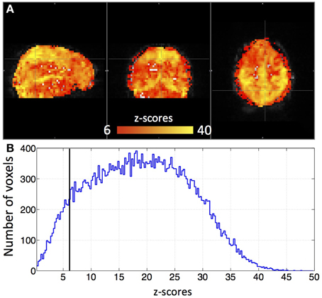
Figure 4. A maximum z-statistic map (A) of the same subject as in Figure 3. The histogram of the maximum z-statistic map is shown in (B), in which, the black line (z = 6) indicates the threshold.

Figure 5 shows results of three group ICAs: using actual resting state data (Figure 5A); using the synthetic data derived from the recursive method (Figure 5B); and using the synthetic data derived from NIRS method (Figure 5C). The eight spatial patterns were selected from each ICA result by spatial correlation (fslcc in fsl, threshold R > 0.25) using a well-known RSN template (Beckmann et al., 2005), including Medial Visual (45, 19, 37 coordinates in MNI152 2 mm³ standard space), Lateral Visual (45, 19, 37), Auditory (45, 65, 35), Sensory Motor (45, 51, 68), Default-mode (45, 32, 47), Executive-control (45, 73, 56), Dorsal Visual (Right, 45, 78, 56) and Dorsal Visual (Left, 45, 78, 56) network. The corresponding ICs were listed in horizontal groups with their corresponding spatial correlation values (calculated with RSN templates) for easy comparison. IC patterns matching well-known RSNs were found with both types of synthetic as well as in the real data. The spatial correlation coefficients with the RSN templates were highest for the real data (R = 0.48–0.86), decreased slightly with the synthetic data derived with the recursive method (R = 0.32–0.6), and reduced further in the synthetic data derived with the NIRS method (R = 0.26–0.42), while still being above the threshold (R = 0.25). Among the ICs from the synthetic data, the ones resembling the Medial, Lateral Visual networks, the Sensory Motor network, the Executive Control network and the Dorsal Visual (L) network have the highest correlation coefficients (R > 0.4). Medial, Lateral Visual networks cannot be individually identified in the results derived from the synthetic data using the recursive method (marked in red box in Figure 5B), while Dorsal Visual networks (L,R) cannot be separated in the results derived from NIRS method (marked in red box in Figure 5C). The asymmetry in RSN patterns [i.e., Dorsal Visual networks (L,R)] detected in the real data, as in Figure 5A, are replaced with the symmetrical ones in the results derived from the synthetic data using the recursive method (Figure 5B). Interestingly, unsymmetrical patterns [i.e., Dorsal Visual (L,R)] was detected in the results derived from the NIRS method (last two in Figure 5C).

FIGURE 5

Figure 5. Eight groups of ICs resulting from group ICA on 11 subjects' real BOLD data (A), synthetic BOLD data derived with the recursive method (B), and synthetic BOLD data derived from NIRS data (C). The eight ICs were selected in each group result (real vs. synthetic) using RSNs templates (Beckmann et al., 2005) and the value in each IC shows the spatial correlation coefficient calculated between that IC and the corresponding RSN from the template. The ICs in the red block are the same IC.

Figure 6 shows that the DMN was detected from the same group of subjects using both real data and synthetic data by seed analyses (seed location is marked by a black circle). The spatial correlation between these two results is R = 0.83.

FIGURE 6

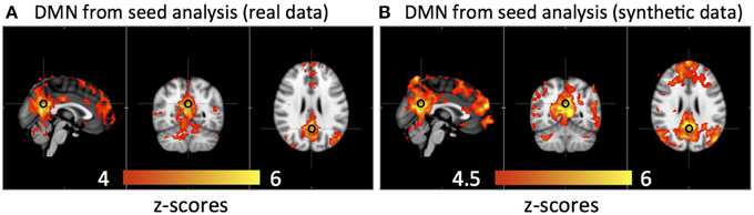
Figure 6. Averaged default mode network detected by seed analysis from 11 subjects' real resting state data (A) and synthetic resting state data (B). Black circles indicate the seed location.

Discussion

ICA is Highly Sensitive to Temporal Shifts in Bold Signal

In this study, we show that the ICA method used in many resting state analyses is sensitive to the temporal shifts in the BOLD signals. The same temporal signal, shifted a few seconds in one direction, can give rise to multiple distinct spatial networks. As shown in Figure 2, five symmetric “networks” are found when the only difference in the voxels is the time shift of an identical signal over a 4 s range. This has somewhat important implications for RSN studies, since the following two conditions: (1) time shifts in the signals; and (2) symmetric distribution of these signals with certain time shifts, are characteristic of the propagating sLFOs, which are prominent in the resting state data of real subjects, as mentioned in the introduction. The concern is that many symmetric artificial networks can be “detected” by ICA along the cerebral blood flow path, even without neuronal contribution. On the same synthetic data set, we tried different time shifts range (instead of 4 s) and found ICA could not separate ICs when the time range is below 0.3 s. This is an empirical result and more theoretical studies are needed to understand the effects of temporal shifts on ICA.

The sLFO Delay Maps can be Derived from Resting State Data

To test this hypothesis on real subjects, we generated synthetic resting state data. The first step was to calculate the subject-specific delay maps from 11 healthy subjects' resting state data. We did this using two different methods.

First, we employed a recursive method that takes advantage of the ultrafast fMRI (TR = 0.4 s) acquisition. The method, which we have previously described in detail (Tong and Frederick, 2014), is designed specifically to accurately assess the temporal shifts between sLFOs from relevant BOLD signals in the brain using resting state data, and avoid neuronal activity. The advantages of this method are: (1) the sLFOs and delay map can be derived directly from fMRI data itself; (2) the procedure is very robust, resulting in similar delay maps regardless of the initial seed selection. However, the method might also be prone to the influence of the global neuronal signals, which we discuss in detail in The Delay Maps Were Calculated to Only Reflect the Temporal Delays of the sLFOs in BOLD Signals.

For the second method, we utilized the fact that sLFOs travel throughout the body (Tong et al., 2012) to calculate the delay map in the brain using the simultaneously recorded NIRS Δ[HbO] at the fingertip. This method is very straightforward, and is likely to give quite accurate delay values. However, there are a few factors, which may reduce the sensitivity of the technique. The NIRS peripheral data catches the essential sLFOs, but it has following caveats: (1) It measures a single point that is far from the brain, which may add noise to the correlation, due to peripheral vascular effects; (2) it is the Δ[HbO] signal, not the direct BOLD signal, so the signal waveform may not exactly match that of the BOLD; (3) it is a static signal, and does not reflect amplitude changes of sLFOs as they propagate through the brain. These may affect its sensitivity in calculating the delay map. However, these delay maps are very straightforward to calculate, and are unequivocally independent of any neuronal signal (these delay maps use a wholly extracerebral signal in calculating the time delays).

As shown in previous studies (Tong and Frederick, 2014), we have demonstrated the dynamic flow patterns obtained from these two methods likely reflect the cerebral blood flow in terms of dynamic spatial distribution and temporal duration (see the Supplementary Movie). This has not yet been fully validated (dynamic susceptibility contrast MRI experiments are being conducted to validate this hypothesis). However, the fact that similar patterns have been derived among subjects using multiple methods demonstrates the robustness of the sLFO effect, indicating its universal existence in the resting state data.

The Delay Maps Were Calculated to Only Reflect the Temporal Delays of the sLFOs in Bold Signals

There are two concerns in calculating these delay maps. One concern is that these delay maps can be biased by the regional spontaneous neuronal signals. Even more, we might introduce some artificial delays, essentially filtering the low frequency fMRI data to the frequency and phase profile of the sLFOs (or of even random timeseries), which were not there in the first place. This is unlikely for the following reasons: (1) these physiological regressors (i.e., sLFOs) are obtained or derived from actual data recorded in the periphery or brain, which have been shown to be highly correlated with the BOLD of the resting state—they are not random, non-related low frequency oscillations; (2) the voxel-wise z-value calculated by these real physiological regressors (using GLM) are statistically significant, as shown in Figure 4A. Figure 4B shows the histogram of these z-values. From these graphs, we observe that the mean z-value calculated at each voxels using the recursive regressors is around 20 (which is the case for all the subjects). As the delay values are only calculated from the voxels that significantly correlated with these regressors (z > 6), we can ensure that the corresponding delay values accurately reflect only the arrival time of these sLFOs, no other signals. On the contrary, correlation with random signals do not generate maps with statistical significance; (3) if the spontaneous neuronal signals do affect the delay map, they should influence the delay map differently across the subjects due to its spontaneous nature. However, the delay map and dynamic patterns derived from different subjects are not random. They mimic the cerebral flow patterns (as shown in the Supplementary Movie) both in spatial pattern and delay times and are very consistent between subjects. A z-statistic map and its corresponding delay map of another subject were shown as Supplementary Figure 2, in which, similar patterns as in Figure 3 (and Figure 4) can be observed. Lastly, we have generated synthetic delay maps with randomly assigned delay values, which did not produce a single meaningful RSN. In short, the delay maps are inherent properties of the resting state data. The estimation methods expose these properties, but do not create them.

The other concern is the possibility that some global neuronal activations might influence the delay map (Olbrich et al., 2009; Scholvinck et al., 2010; Tal et al., 2013). However, this is unlikely for the recursive method. First, the evolution of the regressors is very slow (as shown in Supplementary Figure 1). Any two regressors, with seconds of temporal delays between them, are almost identical to each other. The global neuronal signals would evolve much faster. Second, the dynamic patterns derived as result of these regressors and delay map are similar to the cerebral blood flow pattern (as shown as Supplementary Movie) and last about 7–8 s, which are also too long for the global neuronal signals. Moreover, the ICA with the synthetic data did not produce only one IC resembling a RSN, which would be a reasonable result if a small neuronal signal were included in the method. Many RSN-resembling ICs were found through this method, strongly indicating that the timecourses of these networks are correlated, with phase delays of several seconds, which is not consistent with the features of global neuronal activity. Lastly, it is even less likely that neuronal activity affects the delay maps derived from NIRS data. The sLFO regressors in this case are all extracted from the periphery (i.e., fingertip), where there is presumably no neuronal contamination. Yet, almost all the corresponding ICs (eight from the template) with high spatial correlation (fslcc > 0.25) were detected in the result. Among these ICs, the IC with the asymmetric pattern is particularly interesting [pattern 7 in Figure 5A (Dorsal Visual (R))]. As we know, these patterns could not result from a totally symmetric delay map. We do not fully understand why the delay map from NIRS data is asymmetrical, which led to the asymmetric ICs result. The likely reason is that sLFOs do have small arrival time differences between the two hemispheres (perhaps due to slight differences in the anatomy of the two carotids); however, the recursive procedure suppresses this difference by averaging many voxels to get the next regressor, while the procedure using NIRS data did not.

In summary, the most critical facts we demonstrate are that (1) there are robust internal systemic correlations between BOLD timecourses throughout the brain with time delays of up to several seconds, which are unlikely to be the result of spontaneous neuronal activations; (2) these temporal shifts between sLFOs at relevant voxels are present even when using very different derivation methods, so they are unlikely to be due to an artifact of the processing methodology.

Networks Derived from sLFOs are Similar to the RSNs

The ICA results of the two synthetic datasets (from both the recursive and NIRS methods) show high similarity with those from the real data, as shown in Figure 5. Here we would like to remind the reader that in the synthetic data used here, the only subject specific (i.e., “real”) information is the delay map, which provides the time shifts applied to the identical sinusoid waves in each voxel. The results imply two important facts. First, it shows that the sLFO time shift information alone (delay map), applied to even arbitrary (but identical) timecourses, will result in a number of distinct ICs in ICA, which are highly similar to well-known RSNs. In other words, the actual temporal signal of each voxel is irrelevant in producing these ICs resembling RSNs. This finding is surprising. It is commonly believed that all the neuronal fluctuations happening during the resting state are reflected in the temporal BOLD signals of the voxels. If so, the neuronal activity in different RSNs will result in different temporal BOLD signals between networks, and ICA will identify these neuronal signals and corresponding brain regions (i.e., networks). Here we offer an alternative way to obtain these “networks” with synthetic data, unrelated to the neuronal fluctuations. We show that since ICA is sensitive to the temporal shifts in the signals, it identifies these symmetric brain regions in distinct groups even when the only variable is the temporal shift in each voxel. Second, the reason that these meaningful symmetric RSNs were identified (e.g., all six symmetric RSNs in the Beckmann template), instead of random symmetric patterns, is probably that the cerebral vasculature associated with these networks (e.g., visual network) is likely denser or more complicated in these areas due to their functional importance (Collins et al., 2010). For instance, the vascular density in visual cortex is likely higher due to the importance and complexity of the visual function. These vascular features are reflected in the hemodynamic delay map (i.e., more uniform time delay in these regions), thus leading to the detection of the “networks.” This explains the consistency between the RSNs and specific neuroanatomical system. However, even if this is the case, the identified networks still reflect the local vascular anatomy as result of million years of evolution, rather than spontaneous neuronal fluctuations.

These arguments are not confined to the results of ICA. As we show in Figure 6, similar RSNs (i.e., the DMN) were also detected from both real and synthetic group data derived through seed analysis. It is not as surprising; seed analysis is even more sensitive to the temporal shifts of the data, since the method itself is based on searching regions with high temporal correlations with the seed voxel. The regions with the same time delays of the sLFOs will be detected as “highly correlated,” while the regions with different time delays are not “correlated,” even when all these temporal signals are the same oscillations, differing only in phase (i.e., synthetic data).

These sLFOs-related ICs share many of the characteristics of the RSNs commonly found in resting state studies. For example, the detected networks are robust. Since the basic blood vasculature is stable (which would lead to a stable delay map), it is not surprising that many RSNs are consistently found in many states, including sleep (Deco et al., 2014), sedation (Greicius et al., 2008), and even vegetative state (Vanhaudenhuyse et al., 2010), in many conditions (i.e., depression, schizophrenia), and even in other mammals (Rilling et al., 2007; Zhang et al., 2010a). The small variations found in these networks from different states and populations could also be explained by the corresponding vascular changes, for example, schizophrenia patients are known to have altered blood flow in certain brain regions (Cohen et al., 1995) relative to neurotypical subjects, which would presumably lead to changes in their vascular delay map. Moreover, the existence of stable vascular “networks” offers an intriguing explanation to some somewhat surprising results in the literature. For example many split brain patients maintain a surprisingly high level of interhemispheric coherence as seen in RSN studies (Uddin et al., 2008). While there is a convincing argument to be made for information transfer over extracallosal neuronal pathways, it is also true that callosal surgery is unlikely to disturb the symmetry of vascular arrival times; some of the preservation of bilateral networks may reflect the contribution of these “vascular networks.” Recently, Christen et al. found temporally shifted BOLD signals in the resting state data of Moyamoya patients and disturbed RSN patterns (Christen et al., 2015). These are likely caused by the blocked arteries at the base of the brain, which directly support the argument of vascular network and its effects on RSN detections.

We have demonstrated that purely vascular signals can give rise to spatial networks which match common RSNs. If this is the case, there should be relative delays between these networks that are determined by their relative locations on the vascular “tree.” While there will be individual variation, we would expect that some networks should consistently be “ahead” of certain other networks due to the shorter vascular distance to the arterial root. To test this, for each subject, we extracted the averaged temporal delay for each RSN from the delay map. The results are shown in Figure 7, where each colored line represents one subject's normalized delay trace connecting the eight RSNs' averaged temporal delays (i.e., the networks 1–8 are in the same order as shown in Figure 5). The delay time matrix (with standard deviation of each delay value) is given in the Supplementary Material (for the purpose of display, the error bars are not shown in Figure 7, while the similar graph with error bars is given Supplementary Figure 3 with offsets). From these results, we ran a paired t-test (two tails with 5% confidence level) on each pair of networks to assess their relative temporal relationship. Even when Bonferroni correction was applied to account for the 56 comparisons performed, there were still a number of significant relationships. For example, network 3 (the auditory network) is consistently ahead of network 2 (the lateral visual network) (as shown in Figure 7). In general, networks 3 and 4 (the sensory–motor network) are “early” vascular networks, networks 2 and 5 (DMN) are late ones. Networks 1, 6, 7, and 8 are roughly in the middle with no clear order. These results are strong indications of internal robust temporal relationships between networks. If the delay maps were the results of spurious correlation calculation, we should not find any consistent relationships among networks from 11 subjects. The possible explanations for some networks having clear ranking, while others do not, could be: (1) some networks might lie on the same vascular branch (passage) with clear sequential relationship, while the others are on different ones with similar distance to the root. (2) Some networks are more vascular, while the others are more neuronal. More studies are needed to clarify the issue.

FIGURE 7

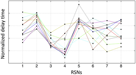
Figure 7. Normalized average temporal delays of each networks (networks 1–8 in the same order as in Figure 5) for each participant. Each color line represents one participant by connecting the average temporal delays of eight networks from this participant.

Interpretation of the Results

In this manuscript, we demonstrate that signals depending only on vascular time delays can generate ICs similar to RSNs through ICA, and offer the argument that these non-neuronal ICs might share some features as commonly attributed to RSNs. To be clear, we are not denying the existence of the neuronal networks. There is ample evidence from other imaging modalities to support the neuronal origin of RSNs. These imaging modalities include the technologies that assess the neuronal activation indirectly, such as positron emission tomography (PET) and arterial spin labeling (ASL) MRI, and those measuring neuronal activation directly, such as electroencephalogram (EEG) and magnetoencephalography (MEG).

PET is sensitive to brain metabolism. The DMN was initially identified by O15-PET to be the areas showing increase in oxygen extraction fraction (i.e., decrease in brain activity) during cognitive tasks (Raichle et al., 2001). Recent FDG-PET studies confirm the existence of many networks, including visual, auditory and motor networks through glucose utilization. However, they were not able to find the DMN (Di et al., 2012). Similar RSNs were identified by ASL that is sensitive to the blood flow changes (Biswal et al., 1997; Zou et al., 2009; Viviani et al., 2011). Like BOLD fMRI, these methods are not a direct measurement of neuronal activities, thus they are still prone to the influence of underlying vascular structure.

However, there is direct evidence of neuronal networks from EEG/MEG studies, which measure the neuronal signal directly. In concurrent EEG/fMRI studies, the data has shown correlations between cortical electrical activity (measured by electroencephalogram) and certain RSNs' slow BOLD oscillations in resting state studies (Martinez-Montes et al., 2004; Hiltunen et al., 2014). Moreover, an independent MEG study has shown good spatial agreement with the RSNs found by fMRI (Brookes et al., 2011). These results offer the direct support of the existence of RSNs of neuronal origin.

One explanation for our finding is the coexistent of both vascular and neuronal networks. There is no reason to believe that vascular networks are fully independent of neuronal function. Their role is to support neurons, thus their structure and development is likely decided by some neuronal factors, such as neuronal density (Collins et al., 2010). As result, the vascular networks are likely overlapping or partially overlapping with the neuronal networks that they serve. Bright et al., found spatially overlapping DMNs of neuronal and physiological origins in task and resting state data (Bright and Murphy, 2014), while Birn et al. found the network similar to DMN using the respiratory regressor (Birn et al., 2006). This evidence supports the hypothesis of overlapping vascular and neuronal networks. Based on these assumptions, we believe that the RSNs detected by ICA or seed analysis in fMRI are likely a mixture of both types of networks. Unfortunately, PET and MEG, especially MEG, have much lower spatial resolution than fMRI, so at the present time their independent RSN results (which are most likely purely neuronal) cannot be used to directly interpret the fMRI results. However, in the recent study on RSNs' changes with age, Balsters et al. used EEG-informed fMRI analyses to separate networks of neuronal origin from those of non-neuronal origin (Balsters et al., 2013).

In terms of signals, the contribution of spontaneous neuronal fluctuations to BOLD fMRI is hard to identify due to large physiological oscillations, and lack of a neuronal task regressor in resting state. Based on our studies, the sLFOs (identified by their time lagged correlation with sLFOs signals) appear to explain ~30% variance in the BOLD signal in gray matter, while respiration and cardiac pulsation could contribute another 10–15% (Chang et al., 2009). There are other physiological processes including motion, CO₂ level, etc. Even with these non-neuronal factors, neuronal fluctuation likely still contributes a considerable amount of signal. To accurately quantify it, however, it is critical to identify and remove various physiological fluctuations.

Future Studies

Effective denoising is critical in RSN studies. There are many denoising methods proposed to remove different physiological signals from the resting state BOLD (Murphy et al., 2013), however for the most part these have treated low frequency oscillations as a epiphenomenon of cardiac and respiratory fluctuations, or as an aliasing artifact. We argue that the sLFO signal must be considered directly as an independent physiological noise source. First, we need to understand the sLFO signal and measure it accurately. We have shown that the sLFOs measured by NIRS at periphery, or derived recursively from the BOLD, are essentially the same traveling signal (Tong et al., 2012), which is different from LFOs derived from models using the respiratory and cardiac signals (Birn et al., 2008; Chang et al., 2009). We have found that sLFOs are major contributors to the BOLD. However, these signals are poorly understood (Sassaroli et al., 2012). The literature attributes them to vasomotion and blood pressure wave (Nilsson and Aalkjaer, 2003), or simply describes them as “Mayer waves” (Julien, 2006), however, no consensus on their origin has been reached.

Second, our results show any denoising method developed needs to incorporate temporal information into the denoising procedure. Many physiological signals such as sLFOs, respiration, and cardiac pulsations, travel with different speeds inside the blood vessels throughout the body. They will arrive at different locations at different times. Using a static regressor, they cannot be effectively removed from the BOLD signals. Our method (Riptide) does characterize the temporal shifts of sLFOs so that they can be removed from the BOLD (Frederick et al., 2012); we continue to refine this method, and other denoising methods also include this type of temporal information (Chang et al., 2009).

As we discussed earlier, multimodality imaging techniques have great advantages, especially when they include EEG or MEG, which measure the neuronal activation directly. However, the experimenter must take care in performing these studies—many multimodality studies probing the spatial or temporal coherence of RSNs have treated the networks derived from fMRI as “the standard” in these comparisons. However, we argue that it is equally important to investigate the spatial and temporal differences, which might elucidate the difference between vascular and neuronal networks.

Conclusion

We believe that this study has two important implications for resting state connectivity analysis. First, we have demonstrated that ICA methods (as well as seed analysis) are sensitive to temporally shifted BOLD signals, and as a result, different “networks” may be identified by ICA even if the only difference between these networks are the temporal shifts in the BOLD. Second, we have shown the possibility that some RSNs can be derived from non-neuronal signals, such as the temporally shifted sLFOs, which are prominent in resting state BOLD fMRI data. This study indicates the importance of fully assessing and removing these sLFOs. Otherwise, the apparent strength and extent of neuronal RSNs will be strongly biased by the hemodynamic information.

Conflict of Interest Statement

The authors declare that the research was conducted in the absence of any commercial or financial relationships that could be construed as a potential conflict of interest.

Acknowledgments

The work was supported by the National Institutes of Health, Grants K25 DA031769 (YT), R21 DA032746 (BF). We thank Dr. Scott Lukas for his support on the project and helpful discussions. We would like to thank the reviewers for their comments, which helped to improve the manuscript considerably.

Supplementary Material

The Supplementary Material for this article can be found online at: https://www.frontiersin.org/article/10.3389/fnhum.2015.00285/abstract

Supplementary Figure 1. Regressors derived from the recursive procedure are plotted in groups (at 3TR = 1.2 s intervals instead of 1 TR) for comparison. Similarities between regressors, especially neighboring regressors are obvious, while progressive changes can also be observed.

Supplementary Figure 2. A maximum z-statistic map (A) and sLFO delay map (B) of a single subject different from the one shown in Figures 3, 4.

Supplementary Figure 3. Normalized average temporal delays of each networks (networks 1–8 in the same order as in Figure 5) for each participant with error bars representing the standard deviations calculated from each network.

References

Balsters, J. H., O'Connell, R. G., Galli, A., Nolan, H., Greco, E., Kilcullen, S. M., et al. (2013). Changes in resting connectivity with age: a simultaneous electroencephalogram and functional magnetic resonance imaging investigation. Neurobiol. Aging 34, 2194–2207. doi: 10.1016/j.neurobiolaging.2013.03.004

PubMed Abstract | CrossRef Full Text | Google Scholar

Beckmann, C. F., Deluca, M., Devlin, J. T., and Smith, S. M. (2005). Investigations into resting-state connectivity using independent component analysis. Philos. Trans. R. Soc. Lond. B Biol. Sci. 360, 1001–1013. doi: 10.1098/rstb.2005.1634

PubMed Abstract | CrossRef Full Text | Google Scholar

Beckmann, C. F., and Smith, S. M. (2004). Probabilistic independent component analysis for functional magnetic resonance imaging. IEEE Trans. Med. Imaging 23, 137–152. doi: 10.1109/TMI.2003.822821

PubMed Abstract | CrossRef Full Text | Google Scholar

Birn, R. M., Diamond, J. B., Smith, M. A., and Bandettini, P. A. (2006). Separating respiratory-variation-related fluctuations from neuronal-activity-related fluctuations in fMRI. Neuroimage 31, 1536–1548. doi: 10.1016/j.neuroimage.2006.02.048

PubMed Abstract | CrossRef Full Text | Google Scholar

Birn, R. M., Smith, M. A., Jones, T. B., and Bandettini, P. A. (2008). The respiration response function: the temporal dynamics of fMRI signal fluctuations related to changes in respiration. Neuroimage 40, 644–654. doi: 10.1016/j.neuroimage.2007.11.059

PubMed Abstract | CrossRef Full Text | Google Scholar

Biswal, B. B., van Kylen, J., and Hyde, J. S. (1997). Simultaneous assessment of flow and BOLD signals in resting-state functional connectivity maps. NMR Biomed. 10, 165–170.

PubMed Abstract | Google Scholar

Biswal, B., Yetkin, F. Z., Haughton, V. M., and Hyde, J. S. (1995). Functional connectivity in the motor cortex of resting human brain using echo-planar MRI. Magn. Reson. Med. 34, 537–541. doi: 10.1002/mrm.1910340409

PubMed Abstract | CrossRef Full Text | Google Scholar

Bright, M. G., and Murphy, K. (2014). “Spatially coupled functional and vascular networks,” in Joint Annual Meeting ISMRM-ESMRMB (Milan).

Brookes, M. J., Woolrich, M., Luckhoo, H., Price, D., Hale, J. R., Stephenson, M. C., et al. (2011). Investigating the electrophysiological basis of resting state networks using magnetoencephalography. Proc. Natl. Acad. Sci. U.S.A. 108, 16783–16788. doi: 10.1073/pnas.1112685108

PubMed Abstract | CrossRef Full Text | Google Scholar

Calhoun, V. D., Adali, T., Pearlson, G. D., and Pekar, J. J. (2001). Spatial and temporal independent component analysis of functional MRI data containing a pair of task-related waveforms. Hum. Brain Mapp. 13, 43–53. doi: 10.1002/hbm.1024

PubMed Abstract | CrossRef Full Text | Google Scholar

Chang, C., Cunningham, J. P., and Glover, G. H. (2009). Influence of heart rate on the BOLD signal: the cardiac response function. Neuroimage 44, 857–869. doi: 10.1016/j.neuroimage.2008.09.029

PubMed Abstract | CrossRef Full Text | Google Scholar

Christen, T., Jahanian, H., Ni, W. W., Qiu, D., Moseley, M. E., and Zaharchuk, G. (2015). Noncontrast mapping of arterial delay and functional connectivity using resting-state functional MRI: a study in Moyamoya patients. J. Magn. Reson. Imaging 41, 424–430. doi: 10.1002/jmri.24558

PubMed Abstract | CrossRef Full Text | Google Scholar

Cohen, B. M., Yurgelun-Todd, D., English, C. D., and Renshaw, P. F. (1995). Abnormalities of regional distribution of cerebral vasculature in schizophrenia detected by dynamic susceptibility contrast MRI. Am. J. Psychiatry 152, 1801–1803. doi: 10.1176/ajp.152.12.1801

PubMed Abstract | CrossRef Full Text | Google Scholar

Collins, C. E., Airey, D. C., Young, N. A., Leitch, D. B., and Kaas, J. H. (2010). Neuron densities vary across and within cortical areas in primates. Proc. Natl. Acad. Sci. U.S.A. 107, 15927–15932. doi: 10.1073/pnas.1010356107

PubMed Abstract | CrossRef Full Text | Google Scholar

Crandell, D., Moinuddin, M., Fields, M., Friedman, B. I., and Robertson, J. (1973). Cerebral transit time of 99m technetium sodium pertechnetate before and after cerebral arteriography. J. Neurosurg. 38, 545–547. doi: 10.3171/jns.1973.38.5.0545

PubMed Abstract | CrossRef Full Text | Google Scholar

Damoiseaux, J. S., Rombouts, S. A., Barkhof, F., Scheltens, P., Stam, C. J., Smith, S. M., et al. (2006). Consistent resting-state networks across healthy subjects. Proc. Natl. Acad. Sci. U.S.A. 103, 13848–13853. doi: 10.1073/pnas.0601417103

PubMed Abstract | CrossRef Full Text | Google Scholar

Deco, G., Hagmann, P., Hudetz, A. G., and Tononi, G. (2014). Modeling resting-state functional networks when the cortex falls sleep: local and global changes. Cereb Cortex. 24, 3180–3194. doi: 10.1093/cercor/bht176

PubMed Abstract | CrossRef Full Text | Google Scholar

Di, X., Biswal, B. B., and Alzheimer's Disease Neuroimaging, I. (2012). Metabolic brain covariant networks as revealed by FDG-PET with reference to resting-state fMRI networks. Brain Connect. 2, 275–283. doi: 10.1089/brain.2012.0086

PubMed Abstract | CrossRef Full Text | Google Scholar

Fox, M. D., Snyder, A. Z., Vincent, J. L., Corbetta, M., van Essen, D. C., and Raichle, M. E. (2005). The human brain is intrinsically organized into dynamic, anticorrelated functional networks. Proc. Natl. Acad. Sci. U.S.A. 102, 9673–9678. doi: 10.1073/pnas.0504136102

PubMed Abstract | CrossRef Full Text | Google Scholar

Frederick, B., Nickerson, L. D., and Tong, Y. (2012). Physiological denoising of BOLD fMRI data using Regressor Interpolation at Progressive Time Delays (RIPTiDe) processing of concurrent fMRI and near-infrared spectroscopy (NIRS). Neuroimage 60, 1913–1923. doi: 10.1016/j.neuroimage.2012.01.140

PubMed Abstract | CrossRef Full Text | Google Scholar

Greicius, M. D., Kiviniemi, V., Tervonen, O., Vainionpaa, V., Alahuhta, S., Reiss, A. L., et al. (2008). Persistent default-mode network connectivity during light sedation. Hum. Brain Mapp. 29, 839–847. doi: 10.1002/hbm.20537

PubMed Abstract | CrossRef Full Text | Google Scholar

Greicius, M. D., Krasnow, B., Reiss, A. L., and Menon, V. (2003). Functional connectivity in the resting brain: a network analysis of the default mode hypothesis. Proc. Natl. Acad. Sci. U.S.A. 100, 253–258. doi: 10.1073/pnas.0135058100

PubMed Abstract | CrossRef Full Text | Google Scholar

Hampson, M., Peterson, B. S., Skudlarski, P., Gatenby, J. C., and Gore, J. C. (2002). Detection of functional connectivity using temporal correlations in MR images. Hum. Brain Mapp. 15, 247–262. doi: 10.1002/hbm.10022

PubMed Abstract | CrossRef Full Text | Google Scholar

Hiltunen, T., Kantola, J., Abou Elseoud, A., Lepola, P., Suominen, K., Starck, T., et al. (2014). Infra-slow EEG fluctuations are correlated with resting-state network dynamics in fMRI. J. Neurosci. 34, 356–362. doi: 10.1523/JNEUROSCI.0276-13.2014

PubMed Abstract | CrossRef Full Text | Google Scholar

Jenkinson, M., Beckmann, C. F., Behrens, T. E., Woolrich, M. W., and Smith, S. M. (2012). Fsl. Neuroimage 62, 782–790. doi: 10.1016/j.neuroimage.2011.09.015

PubMed Abstract | CrossRef Full Text | Google Scholar

Julien, C. (2006). The enigma of Mayer waves: facts and models. Cardiovasc. Res. 70, 12–21. doi: 10.1016/j.cardiores.2005.11.008

PubMed Abstract | CrossRef Full Text | Google Scholar

Martinez-Montes, E., Valdes-Sosa, P. A., Miwakeichi, F., Goldman, R. I., and Cohen, M. S. (2004). Concurrent EEG/fMRI analysis by multiway Partial Least Squares. Neuroimage 22, 1023–1034. doi: 10.1016/j.neuroimage.2004.03.038

PubMed Abstract | CrossRef Full Text | Google Scholar

Matcher, S. J., Cope, M., and Delpy, D. T. (1994). Use of the water absorption spectrum to quantify tissue chromophore concentration changes in near-infrared spectroscopy. Phys. Med. Biol. 39, 177–196. doi: 10.1088/0031-9155/39/1/011

PubMed Abstract | CrossRef Full Text | Google Scholar

Menon, R. S. (2012). The great brain versus vein debate. Neuroimage 62, 970–974. doi: 10.1016/j.neuroimage.2011.09.005

PubMed Abstract | CrossRef Full Text | Google Scholar

Moeller, S., Yacoub, E., Olman, C. A., Auerbach, E., Strupp, J., Harel, N., et al. (2010). Multiband multislice GE-EPI at 7 tesla, with 16-fold acceleration using partial parallel imaging with application to high spatial and temporal whole-brain fMRI. Magn. Reson. Med. 63, 1144–1153. doi: 10.1002/mrm.22361

PubMed Abstract | CrossRef Full Text | Google Scholar

Murphy, K., Birn, R. M., and Bandettini, P. A. (2013). Resting-state fMRI confounds and cleanup. Neuroimage 80, 349–359. doi: 10.1016/j.neuroimage.2013.04.001

PubMed Abstract | CrossRef Full Text | Google Scholar

Nilsson, H., and Aalkjaer, C. (2003). Vasomotion: mechanisms and physiological importance. Mol. Interv. 3, 79–89, 51. doi: 10.1124/mi.3.2.79

PubMed Abstract | CrossRef Full Text | Google Scholar

Niu, H., Khadka, S., Tian, F., Lin, Z. J., Lu, C., Zhu, C., et al. (2011). Resting-state functional connectivity assessed with two diffuse optical tomographic systems. J. Biomed. Opt. 16, 046006. doi: 10.1117/1.3561687

PubMed Abstract | CrossRef Full Text | Google Scholar

Obrig, H., Neufang, M., Wenzel, R., Kohl, M., Steinbrink, J., Einhaupl, K., et al. (2000). Spontaneous low frequency oscillations of cerebral hemodynamics and metabolism in human adults. Neuroimage 12, 623–639. doi: 10.1006/nimg.2000.0657

PubMed Abstract | CrossRef Full Text | Google Scholar

Olbrich, S., Mulert, C., Karch, S., Trenner, M., Leicht, G., Pogarell, O., et al. (2009). EEG-vigilance and BOLD effect during simultaneous EEG/fMRI measurement. Neuroimage 45, 319–332. doi: 10.1016/j.neuroimage.2008.11.014

PubMed Abstract | CrossRef Full Text | Google Scholar

Raichle, M. E., Macleod, A. M., Snyder, A. Z., Powers, W. J., Gusnard, D. A., and Shulman, G. L. (2001). A default mode of brain function. Proc. Natl. Acad. Sci. U.S.A. 98, 676–682. doi: 10.1073/pnas.98.2.676

PubMed Abstract | CrossRef Full Text | Google Scholar

Rilling, J. K., Barks, S. K., Parr, L. A., Preuss, T. M., Faber, T. L., Pagnoni, G., et al. (2007). A comparison of resting-state brain activity in humans and chimpanzees. Proc. Natl. Acad. Sci. U.S.A. 104, 17146–17151. doi: 10.1073/pnas.0705132104

PubMed Abstract | CrossRef Full Text | Google Scholar

Sassaroli, A., Pierro, M., Bergethon, P. R., and Fantini, S. (2012). Low-frequency spontaneous oscillations of cerebral hemodynamics investigated with near-infrared spectroscopy: a review. IEEE J. Sel. Top. Quant. Electron. 18, 1478–1492. doi: 10.1109/JSTQE.2012.2183581

PubMed Abstract | CrossRef Full Text | Google Scholar

Scholvinck, M. L., Maier, A., Ye, F. Q., Duyn, J. H., and Leopold, D. A. (2010). Neural basis of global resting-state fMRI activity. Proc. Natl. Acad. Sci. U.S.A. 107, 10238–10243. doi: 10.1073/pnas.0913110107

PubMed Abstract | CrossRef Full Text | Google Scholar

Schreiber, S. J., Franke, U., Doepp, F., Staccioli, E., Uludag, K., and Valdueza, J. M. (2002). Dopplersonographic measurement of global cerebral circulation time using echo contrast-enhanced ultrasound in normal individuals and patients with arteriovenous malformations. Ultrasound Med. Biol. 28, 453–458. doi: 10.1016/S0301-5629(02)00477-5

PubMed Abstract | CrossRef Full Text | Google Scholar

Smith, S. M., Jenkinson, M., Woolrich, M. W., Beckmann, C. F., Behrens, T. E., Johansen-Berg, H., et al. (2004). Advances in functional and structural MR image analysis and implementation as FSL. Neuroimage 23(Suppl. 1), S208–S219. doi: 10.1016/j.neuroimage.2004.07.051

PubMed Abstract | CrossRef Full Text | Google Scholar

Tal, O., Diwakar, M., Wong, C. W., Olafsson, V., Lee, R., Huang, M. X., et al. (2013). Caffeine-induced global reductions in resting-state BOLD connectivity reflect widespread decreases in MEG connectivity. Front. Hum. Neurosci. 7:63. doi: 10.3389/fnhum.2013.00063

PubMed Abstract | CrossRef Full Text | Google Scholar

Tong, Y., and Frederick, B. (2012). Concurrent fNIRS and fMRI processing allows independent visualization of the propagation of pressure waves and bulk blood flow in the cerebral vasculature. Neuroimage 61, 1419–1427. doi: 10.1016/j.neuroimage.2012.03.009

PubMed Abstract | CrossRef Full Text | Google Scholar

Tong, Y., and Frederick, B. D. (2010). Time lag dependent multimodal processing of concurrent fMRI and near-infrared spectroscopy (NIRS) data suggests a global circulatory origin for low-frequency oscillation signals in human brain. Neuroimage 53, 553–564. doi: 10.1016/j.neuroimage.2010.06.049

PubMed Abstract | CrossRef Full Text | Google Scholar

Tong, Y., and Frederick, B. D. (2014). Tracking cerebral blood flow in BOLD fMRI using recursively generated regressors. Hum. Brain Mapp. 35, 5471–5485. doi: 10.1002/hbm.22564

PubMed Abstract | CrossRef Full Text | Google Scholar

Tong, Y., Hocke, L. M., Licata, S. C., and Frederick, B. (2012). Low-frequency oscillations measured in the periphery with near-infrared spectroscopy are strongly correlated with blood oxygen level-dependent functional magnetic resonance imaging signals. J. Biomed. Opt. 17:106004. doi: 10.1117/1.JBO.17.10.106004

PubMed Abstract | CrossRef Full Text | Google Scholar

Tong, Y., Hocke, L. M., Nickerson, L. D., Licata, S. C., Lindsey, K. P., and Frederick, B. (2013). Evaluating the effects of systemic low frequency oscillations measured in the periphery on the independent component analysis results of resting state networks. Neuroimage 76, 202–215. doi: 10.1016/j.neuroimage.2013.03.019

PubMed Abstract | CrossRef Full Text | Google Scholar

Tong, Y., Lindsey, K. P., and Frederick, B. D. (2011). Partitioning of physiological noise signals in the brain with concurrent near-infrared spectroscopy and fMRI. J. Cereb. Blood Flow Metab. 31, 2352–2362. doi: 10.1038/jcbfm.2011.100

PubMed Abstract | CrossRef Full Text | Google Scholar

Uddin, L. Q., Mooshagian, E., Zaidel, E., Scheres, A., Margulies, D. S., Kelly, A. M., et al. (2008). Residual functional connectivity in the split-brain revealed with resting-state functional MRI. Neuroreport 19, 703–709. doi: 10.1097/WNR.0b013e3282fb8203

PubMed Abstract | CrossRef Full Text | Google Scholar

Vanhaudenhuyse, A., Noirhomme, Q., Tshibanda, L. J., Bruno, M. A., Boveroux, P., Schnakers, C., et al. (2010). Default network connectivity reflects the level of consciousness in non-communicative brain-damaged patients. Brain 133, 161–171. doi: 10.1093/brain/awp313

PubMed Abstract | CrossRef Full Text

Viviani, R., Messina, I., and Walter, M. (2011). Resting state functional connectivity in perfusion imaging: correlation maps with BOLD connectivity and resting state perfusion. PLoS ONE 6:e27050. doi: 10.1371/journal.pone.0027050

PubMed Abstract | CrossRef Full Text | Google Scholar

Watanabe, T., Hirose, S., Wada, H., Imai, Y., Machida, T., Shirouzu, I., et al. (2013). A pairwise maximum entropy model accurately describes resting-state human brain networks. Nat. Commun. 4, 1370. doi: 10.1038/ncomms2388

PubMed Abstract | CrossRef Full Text | Google Scholar

Wise, R. G., Ide, K., Poulin, M. J., and Tracey, I. (2004). Resting fluctuations in arterial carbon dioxide induce significant low frequency variations in BOLD signal. Neuroimage 21, 1652–1664. doi: 10.1016/j.neuroimage.2003.11.025

PubMed Abstract | CrossRef Full Text | Google Scholar

Xu, J., Moeller, S., Auerbach, E. J., Strupp, J., Smith, S. M., Feinberg, D. A., et al. (2013). Evaluation of slice accelerations using multiband echo planar imaging at 3 T. Neuroimage 83, 991–1001. doi: 10.1016/j.neuroimage.2013.07.055

PubMed Abstract | CrossRef Full Text | Google Scholar

Zhang, N., Rane, P., Huang, W., Liang, Z., Kennedy, D., Frazier, J. A., et al. (2010a). Mapping resting-state brain networks in conscious animals. J. Neurosci. Methods 189, 186–196. doi: 10.1016/j.jneumeth.2010.04.001

PubMed Abstract | CrossRef Full Text | Google Scholar

Zhang, Y. J., Lu, C. M., Biswal, B. B., Zang, Y. F., Peng, D. L., and Zhu, C. Z. (2010b). Detecting resting-state functional connectivity in the language system using functional near-infrared spectroscopy. J. Biomed. Opt. 15, 047003. doi: 10.1117/1.3462973

PubMed Abstract | CrossRef Full Text | Google Scholar

Zou, Q., Wu, C. W., Stein, E. A., Zang, Y., and Yang, Y. (2009). Static and dynamic characteristics of cerebral blood flow during the resting state. Neuroimage 48, 515–524. doi: 10.1016/j.neuroimage.2009.07.006

PubMed Abstract | CrossRef Full Text | Google Scholar