A Simple Macroeconomic Model of Decentralized Emission Markets Based on the Solow Growth Model

Introduction

Since the late 20th century, economists have been discussing the role of climate change in growth models, or more precisely, how our societies could sustain long-run economic growth while ensuring the existence of an inhabitable physical realm for such growth to take place (Bryan, 2018). It comes as no surprise that, many economists believe in comparison to increasing the costs of pollution, providing incentives to firms for innovating and improving technology to enhance the “emission efficiency,” is more favorable. Since 1997 when the Kyoto Protocol was signed, in addition to the traditional method of taxation we have become very much used to in the domain of economic policies, the market has also been introduced to carbon trading, or “cap and trade,” where firms would trade their emission quotas (“cap”) in a setting of economic optimization (Carchman, 2014).

Theoretically, such a system should work more efficiently than the carbon tax, in the sense that the introduction of market mechanism would incentivize firms to compete in technology, as those with the highest “emission efficiency” would have the highest quantity of emission quota for trade per unit of the good produced. However, many also start to recognize the problems within this system. From the experiences in the European Union (EU) with their Emission Trading System (ETS), it is clearly observed that depending on the total quantity of quotas set by the government for the industry, the resulting equilibrium carbon credit price could be too low to incentivize the firms to either improve their technologies or switch more technologies “spilled over” from existing firms (Victor, 2009). In this case, the political power of governments is highly constrained as they are not much incentivized to combat industry giants.

When examining this system more closely with the cap and trade policy in Ontario, Canada as an example, we could identify some of the probable causes of such problems. For one, as with the cases in most regions that are utilizing carbon trading, such exchanges only occur between firms within the industry (Ontario Government, 2016). In economics, one could argue that for the general industry, which could be regarded as a representative firm in a model, and it is confined by a fixed quantity of emission quotas albeit the carbon trading system. Hence, as firms make rational decisions, they would aggregately favor investing in political lobbying the governments into maintaining or even expanding the emission quotas than investing an equivalent quantity of capital into improving the technology related with emissions. However, more empirical data and studies would be needed to confirm such arguments.

External Validity of the Model

An Economic Conjecture

While the argument that industries under carbon trading systems lack the internal incentives to allow for the more efficient quantity of emission quotas, is still debatable, many theorists have already come up with an idea about introducing external incentives to this market. In the past decade as the famous Bitcoin’s underlying blockchain technology emerges to be a new trend in the business world, the “decentralized” economy this technology seems to be promising to many is spurring much discussion even within the academic world. One conjuncture brought up not by economists, but more so by enthusiasts in blockchain technology, is about using blockchain to enable carbon trading not only between firms but also between firms and households (Tapscott and Tapscott, 2016).

The general idea is promising: based on blockchain applications such as various forms of smart contracts, governments could build automated auction platforms that allow households to sell their excess emission quotas to the firms. In our research, we would denote such a platform “perfect market of emission quotas,” in contrast to the conventional cap and trade model. The primary differences between them include:

1. In the cap and trade model, emission quotas/credits are only assigned to firms, hence the total quantity of emission quotas available to the industry is restricted to be measured only from the cost functions of the industries, independent of trade; In the perfect emission quotas market, emission quotas are also assigned to households at quantities usually above their consumption demands, which would both include agents with consumption externalities, and derive tradable excess quotas to expand the total quantity of emission quotas available to the industry.

2. In the cap and trade model, transactions in the market primarily take place either privately through negotiations between firms or over emission exchanges at market prices, in a similar manner as many financial instruments exchanged among corporate entities; In the perfect emission quotas market, micro-transactions are conducted automatically on internet platforms; As households list their excess quotas on the platform, they would be sold through automated auctions to the buyers, which would include firms as well as other households.

It needs to be noted at this point that, although we have discussed such a hypothesized market using the notion of blockchain, we have not explicitly treated it as the fundamental technology such a market should be based on, but rather following those who originally have proposed the idea, as an implicit example of the technological improvements that could offer us a market with the necessary traits. Hence, the paper proceeds to suggest that, given these traits, decentralization is the unique technology to support a perfect emission quota market.

An Argument for Decentralization

One of the distinct advantages decentralization technologies offer to markets based on them, is the possibility to decentralize agents from the very transactions they participate in, thanks to the consensus mechanism, which allows for the removal of the inspector who oversees perfect information about the transactions. We would in this section argue that decentralization is crucial for a perfect emission quota market to function as optimized as modeled in later discussion, based on the assumption that the drastically different bargaining powers of the industry and the households would drive the market away from efficient outcomes. Although empirical evidence on such difference specifically in an emission quota market that includes both sides of the economy is lacking, we could observe differences in bargaining powers of the industry and local environment regulatory authorities (Wang et al., 2003), and which derives the intuition about our assumption about the individual households’ relative disadvantage.

Suppose there exists a new technology that is as efficient on the user end in processing transactions as decentralized technologies and based on such a technology an “extended” emission quotas market is formed, which would also effectively achieve to include more agents in the economy whose social welfare are impacted by emissions, and hence the market approaches its competitive equilibrium. However, in the equilibrium (which we would simply refer to as the “efficient outcome” when both production and consumption externalities are internalized for all existing firms and consumers), given the equilibrium price (of emission), the industry has implicit incentive to deviate from it: since the households have little bargaining power compared to the industry, as long as the industry, or the third-party transaction inspector whom the industry can lobby, are able to identify household quota sellers, and firm quota sellers, the industry can optimize its own profit through price discrimination. In addition, although not directly related to the point in this discussion, such a deviation from competitive price due to differences in bargaining powers can also be found between firms of different sizes.

Since the industry always has the incentive to deviate from the competitive price in this superficial centralized market, our hypothesized efficient outcome is not a nash equilibrium this market, and we would eventually observe an inefficient outcome based on differentiated pricing schemes, which may be weakly more efficient than the cap-and-trade model since the households are still included, but definitely far from the perfect emission quota market in our prior discussions. Therefore, it may be argued that to remove the effects of difference in bargaining powers between the industry and households on the emission quota market, disabling the abilities for either party in transactions to identify each other, would be the appropriate approach. It is important to understand at this point that, such anonymity is not just about concealing the names, telephone numbers, and addresses of individual consumers, but more about taking away the capacity for any party to efficiently and systematically determine the types of transaction participants before an automated auction starts, thus it is essential to remove the inspector, or the ledger holder, from the equation.

In addition, another dominant obstacle in the path of transforming the cap and trade model into our perfect market of emission quotas can also be illustrated when we realize the user-end efficiency (while the general economic efficiency varies depending on the types of consensus mechanism) of decentralization technology is still unique compared to most standard implementable technologies today. With conventional technologies, the searching cost, transaction cost as well as the validation cost measured on both time and resources would be too high for such a system to become efficient. On the one hand, a non-blockchain platform may not be able to execute such automated micro-auctions as efficiently as blockchain applications could. On the other hand, even if we could simulate such applications on some conventional internet platforms, the risks on privacy as well as fraudulent transactions would be much higher than those processed on a blockchain settlement. For now, the denoted perfect market of emission quotas seems to be only able to actualize with the use of blockchain technology, more specifically its advantages in consensus mechanism, in the absence of which the marginal costs of this hypothesized system would be higher than the provisioned marginal benefits.

Assumptions and Implications

Drawing on the arguments in the previous section, we would model a decentralization-technology-based perfect emission quota market, by first making a few economic assumptions to ensure the model can be both simple enough for the scope of this paper and internally valid:

1. The quantity of quotas assigned to the representative firm is exogenously set at an initial level that does present an actual obstacle in profit optimization in contrast to the aforementioned EU case; However, that assigned to the representative household would exceed its demand, as explained previously. Note that the governments decreasing the total quantity of quotas assigned to the industry and expand that of the households is purely exogenous, and whether such incentives could actualize under certain political circumstances is not the focus of this study.

2. The number of emission quotas assigned to each household could be determined by many exogenous factors, such as the number of effective labor units and their dependent agents. Since household consumption was originally not the primary source of pollution, setting the household emission quotas above their usual demands effectively allows them to sell their excess quotas on the market, while encouraging them to reduce their own emissions through granting economic incentives.

3. Due to the introduction of blockchain technology, we ignore the searching and transaction costs in our model by arguing that the consensus mechanism would reduce them to levels that are ignorable on aggregate levels (the dominant reason such a system would exist), and we assume both parties involved in the automated auctions enjoy perfect information about their own costs and utilities.

4. We assume that in the general level of technology devoted to production in this economy, only a fraction (or with a multiplier) is devoted to reducing emissions, which means the effect of such emission-reduction technologies is equivalent to increasing production of the industry given the same emission constraint.

As argued earlier, the role of decentralization technology in this model is to enable a hypothetical perfect market of emission quotas, where both the firm and the household would trade toward competitive equilibrium in the quotas market without external costs in acquiring information or waiting for exchanges to be confirmed by third parties. Given such an equilibrium can be supported with the unique assumptions based on decentralization, we would let blockchain reside in the background of our analysis from the next section on. While there indeed exists a variety of blockchain-based applications and consensus mechanisms (proof of work, proof of stake, and etc.), our model does not focus on whether any of these specific applications could actualize the market conditions we desire, but on if the actualized market conditions could, in fact, and lead to sustained economic growths while acting within the emission constraints.

Moreover, it is implicitly assumed that any decentralization technology satisfying the requirement to remove the effects of bargaining power differences in the perfect emission quotas market would suffice for the model. It can even be argued that we would extend the notion of decentralization technology from blockchain in this case, especially as many would suggest, “most of the proposed benefits of so-called blockchain technologies do not really come from elements unique to blockchain” (Halaburda, 2018), albeit so far only the blockchain applications seem to have fit our needs. Hence, it should be kept in mind in our further studies that, when considering our model of a decentralized market, and its potential benefits and risks would not be confined by what has been observed from the contemporary blockchain derivatives today.

In the next section, we would construct a basic macroeconomic model based on capital accumulation and long-run convergence to steady states, to draw some preliminary observations on the effects the adoption of a perfect emission quota market would have on production in the long run and proceed to discuss some possible implications on the short-run economy.

The Mathematical Approach

In order to construct a mathematical model for illustrating the hypothesized perfect market of emission quotas, we start from the conventional Solow-Swan model (Solow, 1956; “Solow model” as the abbreviation in the rest of our discussion). Our tasks are:

1. To examine how the existence of emission quotas would affect an economy’s long-run convergence to the steady-state.

2. To examine the effects of opening trade of emission quotas, not only in the industry but also between both firms and households.

3. To simulate the dynamics of the emission quotas market as capital accumulates, and to find the long-run equilibrium in this market.

The Solow Model

Our basic assumptions follow the Solow model: The intensive-form production function y = f(k) is induced from k = K/AL,y = Y/AL, and f(k) = F(K,AL)/AL where A denotes the efficiency units per labor unit, representing the general technological progress, or R&D sector in the economy; s denotes the saving rate, n denotes the populate growth rate, g denotes the technological growth rate, and δ denotes the capital depreciation rate. As shown in Figure 1, the steady-state in the economy without the presence of emission quotas is at [k^∗,f(k^∗)], or equivalently (k^∗,y^∗); As the economy starts at a level of k lower than its steady-state, it converges to the steady-state over time as capital per effective labor unit accumulates.

FIGURE 1

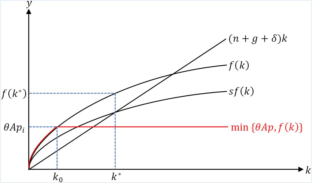
Figure 1. Solow model with aggregate emission quotas.

However, as we consider the implementation of emission quotas, more boundaries need to be defined. We would define P (standing for “pollution”) to be the total amount of emission quotas the entire industry in this economy has measured in units of goods produced. In this case, P functions as a constraint on the production in this economy, as the industry cannot produce more than what it is allowed to. Hence, we could write the production function with the presence of emission quotas as following:

$$y=\min \{\mathrm{\theta }Ap,f\left(k\right)\}(1)$$

Where p = P/AL, denoting the emission quotas per effective labor unit in the economy; θ denotes how specialized in emission-reduction technology the economy is, in its general R&D sector; Then θAp would denote the “effective emission quotas” the industry has at any given point in time. It would seem obvious that: since Solow model assumes a natural progression of technology represented by g the effective emission quotas would increase over time; and that as the economy invests more in developing “clean technologies,” meaning that more focus on emission reduction is given in the R&D sector, θ would also increase to raise the number of effective emission quotas. These points would be considered later.

Meanwhile, for the purpose of our discussion, we assume that in the absence of trade, θ should always be set below f(k^∗), as quotas would be meaningless if their total quantity exceeds the equilibrium production, and which in this case is the steady-state production:

$\mathrm{\theta }Ap\le f\left(k^{*}\right)(2)$

As shown in Figure 1, the new production function (1) essentially caps the original production function at y = θAp_i, where p_i is the initial level of emission quotas the industry is assigned before the trade is available. Intuitively, as the economy starts at any point on f(k) below θAp_i, it would attempt to converge to f(k^∗) but stops at θAp_i as the industry’s emission quotas are totally exhausted. The economy would only continue to grow if θAp increases.

Now we need to analyze how the implementation of trade would impact the economy. Before a trade is available, the total amount of emission quotas available for production equals the total amount the industry is granted by the authority, denoted by ${\overline{P}}_{\text{F}}$ (F stands for the firm, as in the case of a representative firm), hence $P_{\text{i}}={\overline{P}}_{\text{F}}$, and $p_{\text{i}}=\frac{{\overline{P}}_{\text{F}}}{AL}$. Following our prior contexts, we assume the households in our economy are assigned a total quantity of emission quotas in units of goods consumed, denoted by ${\overline{P}}_{\text{H}}$, which is by assumption higher than the total household consumption, which is (1−s)F(K,AL). Note that in this case we actually make the assumption about a one-to-one relationship between household consumption units and emission units; Since we already use technological multipliers θ and A to measure the efficiency of emission units in production, this assumption is without loss of generality.

Equilibrium in the Emission Quotas Market

As trade becomes available, the households sell their excess emission quotas ${\overline{P}}_{\text{H}}-\left(1-s\right)F(K,AL)$ in a hypothesized market with perfect information. Following our assumption that the entirety of excess household emission quotas is not enough to satisfy the industry’s long-run steady-state demands, the excess household emission quotas are always sold out, and the total emission quotas available to the industry becomes:

$P={\overline{P}}_F+\left[{\overline{P}}_H-\left(1-s\right)F(K,AL)\right](3)$

We transform variables in Eq. (2) into intensive form by dividing both sides of the equation by AL:

$\frac{P}{AL}=\frac{{\overline{P}}_F+{\overline{P}}_H}{AL}-\left(1-s\right)\frac{F(K,AL)}{AL}(4)$

Since ${\overline{P}}_F$, ${\overline{P}}_H$, and L are exogenous variables, we can set $B=\frac{{\overline{P}}_F+{\overline{P}}_H}{L}$, where B acts as a constant:

$p=\frac{B}{A}-\left(1-s\right)f\left(k\right)=\frac{B}{A}-\left(1-s\right)y(5)$

Following Eqs (1) and (2), the long-run potential production that the economy can converge to, as restricted by the new p is:

$f{\left(k\right)}_{potential}=\mathrm{\theta }Ap(6)$

Denote the potential long-run production by $\widehat{y}$:

$p=\frac{\widehat{y}}{\mathrm{\theta }A}(7)$

Therefore, we have Eq. (5), which explains the relationship between current production, and current after-trade emission quotas available for production, and Eq. (7), which explains the relationship between current after-trade emission quotas available and its induced potential long-run production capacity. We could denote the former as S_p, or the “supply of emission quotas from the current production,” and then later as D_p, or the “demand of emission quotas from the future production”:

$\{\begin{array}{c}\hfill S_p=\frac{B}{A}-\left(1-s\right)y\hfill \\ \hfill D_p=\frac{\widehat{y}}{\mathrm{\theta }A}\hfill \end{array}(8)$

These two relationships are illustrated in the left domain of Figure 2, where the x-axis and y-axis are inverted for comparison with the production curve from the Solow model.

FIGURE 2

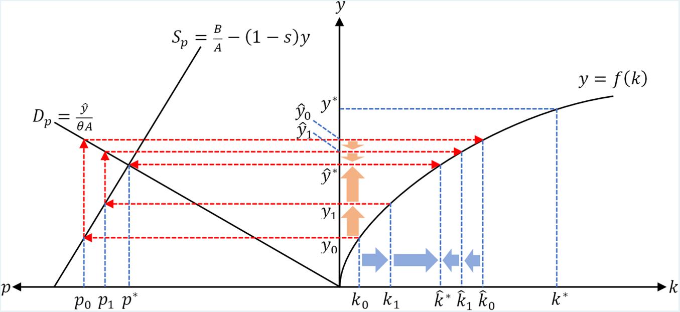
Figure 2. Equilibrium in the emission quotas market.

In Figure 2, consider the economy starting at (k₀,y₀). As trade becomes available, the current production level y₀ induces the current total emission quotas level p₀ on the S_p curve, and which then satisfies the demand from future potential production level ${\widehat{y}}_0$ on the D_p curve. Intuitively, trade allows the constraint on production to be raise from y₀ to ${\widehat{y}}_0$, hence production in the short run would start to grow and converge to ${\widehat{y}}_0$.

However, as capital accumulates from k₀ to k₁ and production rises from y₀ to y₁ when the economy grows, the current total emission quotas level would be lowered from p₀ to p₁ on the S_p curve, and which then satisfies a lower demand from future potential production level ${\widehat{y}}_1$ on the D_p curve. Intuitively, as the economy grows, households increase their consumptions well as the corresponding emission, which results in a decrease of the excess household emission quotas available for trade in the quotas market, hence eventually decrease the total emission quotas available to the industry.

As the current production rises and potential long-run production decreases, the production in the economy would eventually converge to a point above y₀ and below ${\widehat{y}}_0$, which, as shown in Figure 2, is at $({\widehat{k}}^{*},{\widehat{y}}^{*})$, where ${\widehat{y}}^{*}$ is located at the intersection of S_p and D_p curves, and correspondingly the equilibrium amount of emission quotas is denoted by p^∗ at this point. Therefore, in the current stage of our discussion, without accounting for the effects of technological changes, and the long-run equilibrium in emission quotas market is at $({\widehat{y}}^{*},p^{*})$.

Dynamic Analysis of Equilibrium

Now we need to consider the changes in technological factors, specifically A. As an assumption in the Solow model, technology in an economy naturally progresses with a constant growth rate of g. As illustrated in Figure 3, when A increases over time, S_p curve shifts down since its vertical intercept $\frac{B}{A}$ decreases, and D_p curve becomes flatter since its slope $\frac{1}{\mathrm{\theta }A}$ decreases. Then as A increases from A₀ to A₁, and then to A₂, both ${\widehat{y}}^{*}$ and p^∗ continue to decrease.

FIGURE 3

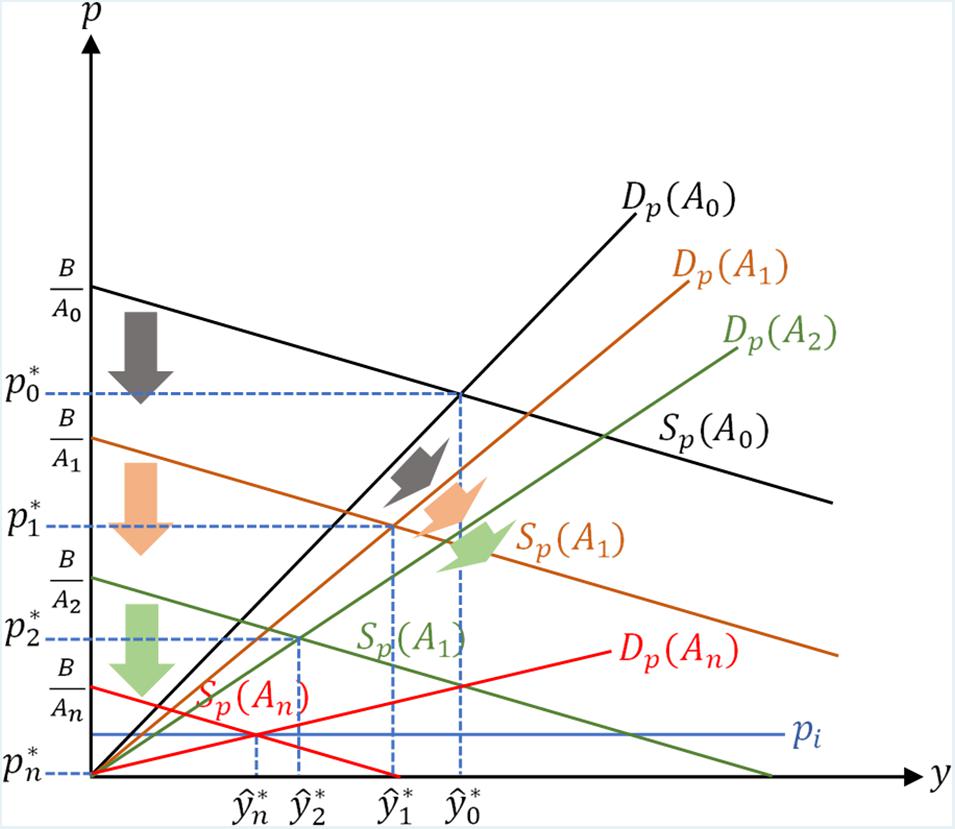
Figure 3. Dynamics of equilibrium with technological changes.

Intuitively, as technology advances, the industry is able to increase production with the same quantity of emission quotas, but at the same time as technological progress raises production, which translates to a higher level of consumption, the available emission quotas also decrease; The effect of reduced emission quotas surpasses the effect of improved emission efficiency, and results in a net decrease of the equilibrium production level.

Hypothetically, as technology continues to advance in the long run, which is represented by an A_n, where D_p curve and S_p curve would intersect the horizontal line p = p_i. At this point there are no excess household emission quotas to be traded in the market, hence the number of emission quotas available to industry returns to its pre-trade amount p_i, and S_p curve ceases to shift down since the emission quotas market has effectively shut down.

However, as technology continues to advance further, D_p curve would continue to become flatter and approximate a horizontal line as the time approaches infinity, which results in a continuous rightward shift of the intersection between D_p curve and the horizontal line p = p_i; Intuitively, the industry is able to utilize its initially assigned emission quotas p_i more effectively, and the equilibrium production in the economy would gradually increase again. It should be noted that this increase in production due to technological progression would take place whether or not the trade of emission quotas is available.

To find the relationship between equilibrium production ${\widehat{y}}^{*}$ and technology multiplierA, we set D_p = S_p at their intersection, where$y=\widehat{y}={\widehat{y}}^{*}$:

$\frac{{\widehat{y}}^{*}}{\mathrm{\theta }A}=\frac{B}{A}-\left(1-s\right){\widehat{y}}^{*}(9)$

Which would give us the ${\widehat{y}}_M^{*}$ curve (M stands for “Market”):

${\widehat{y}}_M^{*}=\frac{B}{\frac{1}{\mathrm{\theta }}+\left(1-s\right)A}(10)$

To find its gradient at A, we test its first-order condition:

$\frac{\partial {\widehat{y}}_M^{*}}{\partial A}=\frac{-B\left(1-s\right)}{{\left[\frac{1}{\mathrm{\theta }}+\left(1-s\right)A\right]}^2}<0(11)$

The first-order condition corresponds to our earlier analysis, that as A increases, ${\widehat{y}}^{*}$decreases. However, we also need to consider the intersection between D_p curve and the horizontal line p = p_i, which gives us the dynamics of ${\widehat{y}}^{*}$ induced by A after tradable emission quotas diminish. In order to do so, we substitute p = p_i into Eq. (7):

$p_i=\frac{{\widehat{y}}^{*}}{\mathrm{\theta }A}(12)$

Which would give us the ${\widehat{y}}_N^{*}$ curve (N stands for “Non-market”):

$${\widehat{y}}_N^{*}=\mathrm{\theta }{p}_{i}A(13)$$

We set $(\tilde{A},\tilde{y})$ to be the technology and production when the tradable emission quotas become 0, then we have the ${\widehat{y}}^{*}$ curve defined overA ∈ (0, + ∞):

${\widehat{y}}^{*}=\{\begin{array}{c}\hfill \frac{B}{\frac{1}{\mathrm{\theta }}+\left(1-s\right)A},A\in (0,\tilde{A})\hfill \\ \hfill \mathrm{\theta }{p}_{i}A,A\in (\tilde{A},+\mathrm{\infty })\hfill \end{array}(14)$

We illustrate Eq. (14) in Figure 4:

FIGURE 4

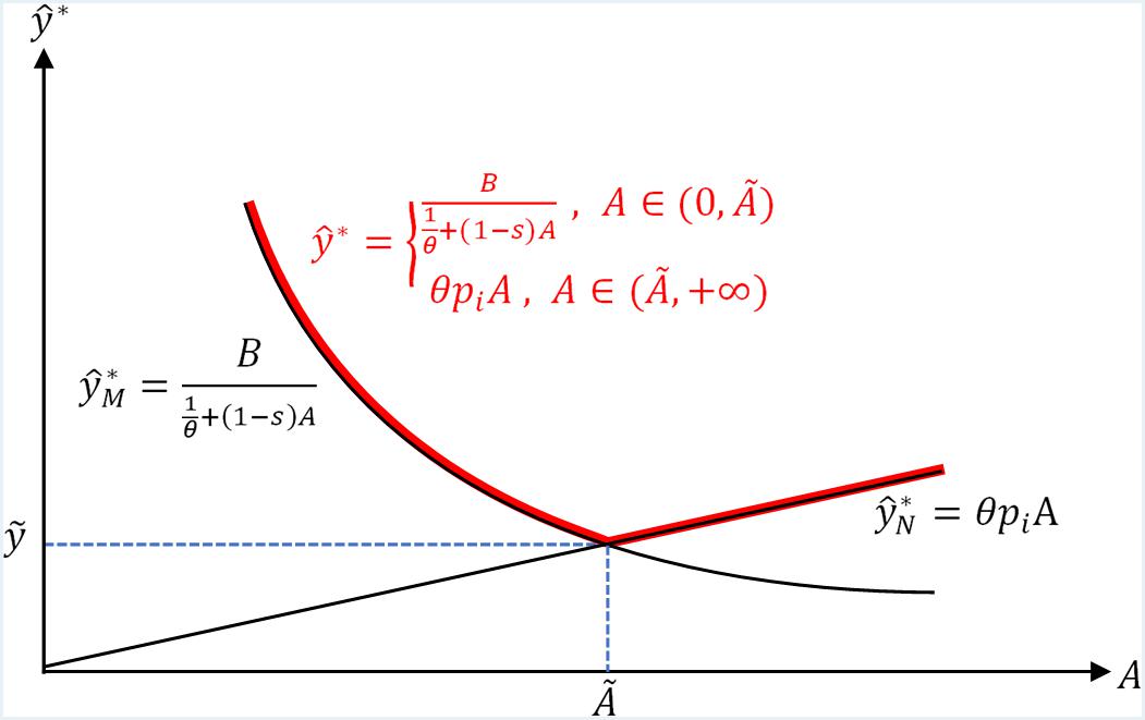
Figure 4. Long-run convergence of equilibrium.

As shown in Figure 4, the piecewise ${\widehat{\text{y}}}^{*}$ curve inflects at $(\tilde{A},\tilde{y})$, at which point the function is non-differentiable, and the emission quotas market shuts down. Without the presence of emission quotas market, the ${\widehat{\text{y}}}^{*}=\mathrm{\theta }{p}_{i}A$ curve would illustrate how technological improvements would raise production over time. Therefore the implementation of emission quotas market allows the economy to expand both production and correspondingly household consumption in the short run, but in the long run, the market would diminish as no excess household emission quotas are available for trade, hence the economy returns to its pre-trade technology-emission growth path, and represented by the ${\widehat{\text{y}}}^{*}=\mathrm{\theta }{p}_{i}A$ curve.

Although intuitively we could conclude from the piece-wise technology-production curve with the presence of emission quotas, that the implementation of perfect emission quotas market cannot induce long-run economic growths, we do recognize its ability to both stimulate short-run economic growths, and more importantly as discussed before, to redistribute wealth in society as firms purchase emission quotas from the households, which could be further discussed in the realm of economic policies on how it would impact social welfare, and if it would what are the magnitudes of such impacts depending on the factors in our model. Given further chances of study, another topic to be explored is the precise timeframe an economy would arrive at $\tilde{A}$, as from such information, we would be able to determine whether or not the seemingly beneficial short-run growth is meaningful to the economy.

Exogenous Adjustments in Technology Multiplier

Based on our current model, we should consider the exogenous change in technology, or the R&D sector, more specifically the increase of investment in emission-reduction-oriented technologies. In our model, such a change is represented by an increase inθ, which represents how effective the general technology in the economy denoted by A is at the specific task of reducing emission in production. We would like to analyze how an increase in θ would affect the ${\widehat{\text{y}}}^{*}$ curve as shown in Eq. (14). In order to complete this task, we would examine the effects such a change would have on the inflection point$(\tilde{A},\tilde{y})$, which is geometrically the intersection point of ${\widehat{\text{y}}}_M^{*}$ curve and ${\widehat{\text{y}}}_N^{*}$ curve, where we set $A=\tilde{A}$, $y=\tilde{y}$:

$\mathrm{\theta }{p}_i\tilde{A}=\frac{B}{\frac{1}{\mathrm{\theta }}+\left(1-s\right)\tilde{A}}(15)$

Solving the equation for $\tilde{A}$ through the quadratic formula:

$\tilde{A}=\frac{-p_i+{\left[p_i^2+4B\left(1-s\right)p_i\mathrm{\theta }\right]}^{\frac{1}{2}}}{2\left(1-s\right)p_i\mathrm{\theta }}(16)$

And correspondingly we can solve for$\tilde{y}$:

$$\tilde{y}=\mathrm{\theta }{p}_i\tilde{A}=\frac{-p_i+{\left[p_i^2+4B(1-s)p_i\mathrm{\theta }\right]}^{\frac{1}{2}}}{2(1-s)}(17)$$

To find the effects of changing θ, we find the first-order conditions of both Eqs (16) and (17) with respect to θ. For the clarity of the presentation of the results, we set:

$\text{x0394;}\left(\mathrm{\theta }\right)={\left[p_i^2+4B\left(1-s\right)p_i\mathrm{\theta }\right]}^{\frac{1}{2}}>0(18)$

And the first-order conditions would be presented as:

$$\{\begin{array}{c}\hfill \frac{\partial \tilde{A}}{\partial \mathrm{\theta }}=\frac{\left\{\text{Δ}{\left(\mathrm{\theta }\right)}^{-1}\left[2B\left(1-s\right)\mathrm{\theta }\right]+1\right\}{p}_i-\text{Δ}\left(\mathrm{\theta }\right)}{2\left(1-s\right)p_i{\mathrm{\theta }}^2}\text{⋛}0\hfill \\ \hfill \frac{\partial \tilde{y}}{\partial \mathrm{\theta }}=\text{Δ}{\left(\mathrm{\theta }\right)}^{-1}B{p}_i>0\hfill \end{array}(19)$$

The first-order conditions suggest that, as we exogenously increase θ, the inflection point production $\tilde{y}$ increases unambiguously, while the inflection point technology $\tilde{A}$ changes ambiguously as the sign of its gradient is dependent on other factors in the model. Using the inflection point as the benchmark, we could geometrically illustrate the effects of changing θ in Figure 5, in which the left and right panels show the different scenarios of decreased and increased inflection point technology$\tilde{A}$, respectively.

FIGURE 5

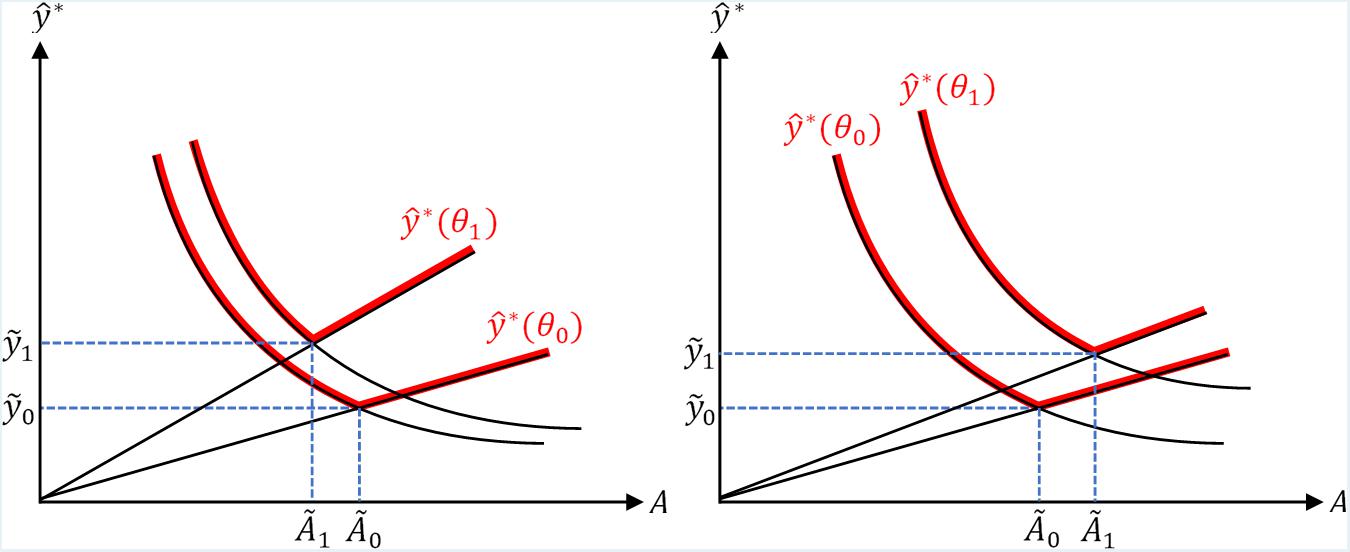
Figure 5. Impacts of technology multiplier shocks.

As shown in Figure 5, in contrast to the effects of opening trade of emission quotas discussed previously, exogenously increasing research and development in emission-reduction-specific technology can induce long-run economic growths, and represented by the upward shift of the ${\widehat{\text{y}}}^{*}$ curve in both scenarios. The intuition is that, if two economies adapt emission quotas that are equivalent in units of good production, one that is more specialized in developing “clean technologies,” independent of the existence of an emission quotas market, would experience higher long-run economic growths.

Summary and Remarks

In summary, we started from the conventional Solow model with a few assumptions about emission quotas market and decentralization, and derive from it the current supply and future demand curves in the emission quotas market, in order to find the long-run market equilibrium regarding the eventual economic growths to be attained when all excess emission quotas supplied by households exhaust; We then considered the exogenous technological changes in the economy, which was also illustrated in the original Solow model, as in how much progress over time would further shift the long-run equilibrium in the perfect emission quotas market; Finally, we arrived at the intuition that, in the long run as technology progresses, the market for emission quotas between households and firms would not only exhaust but also forces the number of quotas available to the industry to diminish to its original state.

Without considering exogenous shocks to technology, our conclusive intuition about the technology-production curve derived was that the presence of perfect emission quotas market would only induce economic growths in the short run, but unable to achieve long-run economic growths. However, one important remark about such a conclusion, is that we have been assuming household emission as well as household consumption both grow linearly with the aggregate production, which is the critical factor behind the diminishing emission quotas market in out study. Intuitively, such an assumption may not be realistic as unless the population also grows linearly with aggregate production, emission-inducing household consumption is most likely confined by the natural consumption limits of human beings. In addition, considering other factors such as economies of scale, in further studies it would be interesting to explore how a household consumption factor with a diminishing gradient would impact our model.

Another remark to be made about this topic given the endogenous dynamics is to emphasize that what this model has illustrated so far about the emission quotas market, is built on the assumption about the existence of an efficient firm-household quotas market. As discussed previously, the conjecture is that blockchain technology, more specific applications that allow for automated and decentralized micro-auctions compensating for the differences in bargaining powers of the industry and the households, would actualize such a market with reasonable marginal costs. However, in time blockchain may prove not to be the most appropriate technological foundation for our discussed perfect emission quotas market, as the general concept of “decentralization” may be achieved through more efficient instruments. Thus, the model of ours is merely an illustration of the possible economic functioning of this hypothetical market, but not strictly bound to the underlying technology that could realize it.

Combining with our observations about the equilibrium dynamics and the analysis of exogenous technological changes, we would emphasize that technology seems to be the determinant factor derived from this model. Such a result partially corresponds to most theories within the framework of neoclassical economics emphasizing capital accumulation and conditional convergence, non-surprisingly as well have followed the Solow growth model. It should be noted that although we have been using the technology factor A as the driving variable in the later sections of this analysis, it is still kept exogenous unlike that in endogenous growth theories, as we are still assuming a natural growth to the general technology factor A along the time horizon, and an exogenous specialization multiplier θ denoting the portion of said general technology dedicated to reducing emission. In any further studies based on this preliminary model, since technology is proven to be a critical factor, it is worth including technology as an endogenous factor according to capital and labor inputs in the R&D sector, and the specialization multiplier could be kept exogenous, or included as endogenous as well. By examining the effects of the emission quotas market in an endogenous growth model, we could determine if it has any benefits or risks that are not observed from our current analysis.

Given the scope of this model, albeit rather preliminary as the contemporary literature, as well as the corresponding empirical observations, are yet to be regarded as profound, the observations and speculations are still interesting to inspire further researches based on more evidence and experience with the application of the technologies associated. While the long-run analysis has not derived results far from conclusions from most neoclassical growth models, mostly due to the fundamental constraints of capital accumulation and emission themselves, we should note in the short run optimizing the structure of the emission regulations should bring benefits to both aggregate levels of production as well as social welfare as the inclusion of households could shift the emission market toward competitive equilibrium, as globalization has done to a certain degree the commodity and capital market of the world.

And finally, as being one of the few merits of this study, one would realize that blockchain technologies, and more importantly the ideology of decentralization, are closely related to economic studies. In the next decades, if such technological trends would not prove to be mere bubbles, they could become a transformative force, either constructive or destructive, in our economies in terms of how markets would be fundamentally structured. As mentioned previously literature within this field are still relatively a minority, hence more intricate works would be done in the near future on this topic.

Data Availability Statement

The raw data supporting the conclusions of this article will be made available by the authors, without undue reservation, and to any qualified researcher.

Author Contributions

All authors contributed to the manuscript significantly either in writing, research, or communication. The ordering of the authors signifies the relative contribution of all author.

Conflict of Interest

The authors declare that the research was conducted in the absence of any commercial or financial relationships that could be construed as a potential conflict of interest.

References

Bryan, K. (2018). How We Create and Destroy Growth: The 2018 Nobel Laureates. London: VOX, CEPR Policy Portal.

Google Scholar

Carchman, M. (2014). A BRIEF History of the Global Carbon Market. Bourne End: ADEC Innovations.

Google Scholar

Halaburda, H. (2018). Blockchain Revolution Without the Blockchain. Bank of Canada Staff Analytical Note 2018-5. Avaliable online at: https://ssrn.com/abstract=3133313 (accessed December 1, 2018).

Google Scholar

Ontario Government (2016). Cap and Trade in Ontario. Ministry of the Environment, Conservation and Parks. Avaliable at: https://www.ontario.ca/page/cap-and-trade-ontario (accessed December 2018)Google Scholar

Solow, R. (1956). A contribution to the theory of economic growth. Q. J. Econ. 70, 65–94. doi: 10.2307/1884513

CrossRef Full Text | Google Scholar

Tapscott, D., and Tapscott, A. (2016). Blockchain Revolution: How the Technology Behind Bitcoin Is Changing Money, Business, and the World. New York, NY: Portfolio.

Google Scholar

Victor, D. (2009). The Problem with Cap and Trade. Cambridge: MIT Technology Review.

Google Scholar

Wang, H., Mamingi, N., Laplante, B., and Dasgupta, S. (2003). Incomplete enforcement of pollution regulation: bargaining power of chinese factories. Environ. Resour. Econ. 24, 245–262. doi: 10.1023/A:1022936506398

CrossRef Full Text | Google Scholar