Empirical assessment of non-linear seismic demand of mainshock–aftershock ground-motion sequences for Japanese earthquakes

Introduction

Ground-motion records are the main source of uncertainty in predicting non-linear responses of structures subjected to earthquake loading. Key record features can be represented by amplitude, duration, frequency content, and their temporal evolution. They are influenced by physical environments and characteristics, such as earthquake type (crustal/interface/inslab), moment magnitude (M_w), faulting mechanism, stress drop, seismic wave propagation, and local site condition (Stein and Wysession, 2003). In the last decade, observation networks of strong motion around the world have been expanded significantly, and numerous recordings have been made available publicly, e.g., K-NET/KiK-net in Japan, TSMIP in Taiwan, GeoNet in New Zealand, and ITACA in Italy. These databases facilitate the development of new generations of empirical ground-motion prediction equations that are essential for probabilistic seismic hazard analysis (e.g., Morikawa and Fujiwara, 2013). Moreover, they are useful for developing inelastic seismic demand prediction models (e.g., Ruiz-García and Miranda, 2003; Vamvatsikos and Cornell, 2004; Federal Emergency Management Agency, 2005; Iervolino and Cornell, 2005). The integration of seismic hazard and ground-motion models with seismic vulnerability models results in a comprehensive performance-based earthquake engineering (PBEE) framework that accounts for main sources of uncertainty related to seismic damage assessment and loss estimation (Cornell et al., 2002; Goulet et al., 2007).

Recent earthquake disasters highlight that a cluster of major aftershocks causes incremental damage to structures whose seismic capacities may have been reduced by a mainshock and poses significant risk to evacuees and residents in a post-disaster situation. For instance, the 2011 Christchurch aftershock sequence (notably the 22 February 2011 M_w6.2 event), initiated by the 2010 M_w7.0 Darfield event, caused extensive damage to buildings and infrastructure in downtown Christchurch (Smyrou et al., 2011). After the 2011 M_w9.0 Tohoku earthquake in Japan, numerous aftershocks as large as M_w7.9 were observed, and additional structural damage and disruption to utility services were caused by major aftershocks (Goda et al., 2013). In Indonesia, regional seismic activities have been heightened since the 2004 M_w9.3 Sumatra earthquake (Shcherbakov et al., 2013). Numerous moderate-to-large earthquakes occurred and caused major seismic damage to structures in Sumatra (e.g., 2005 M_w8.6 and 2007 M_w8.5 events). To evaluate seismic responses of different structures (i.e., steel, concrete, and wood-frame buildings) due to mainshock–aftershock (MS–AS) sequences, various models, such as single-degree-of-freedom (SDOF) and multi-degree-of-freedom systems with different hysteretic models, have been used (e.g., Li and Ellingwood, 2007; Moustafa and Takewaki, 2010; Goda, 2012; Ruiz-García, 2012; Zhai et al., 2013). The developed seismic demand models for MS–AS sequences can be incorporated into the PBEE framework to account for seismic damage and loss caused by aftershocks (Salami and Goda, 2014).

In Japan, national and regional strong-motion networks, K-NET/KiK-net¹ and SK-net², have been established aftermath the 1995 Kobe earthquake. The availability of strong-motion records in Japan has increased drastically and numerous invaluable data have been recorded. One of the events that are extremely well-recorded is the 2011 M_w9.0 Tohoku earthquake; more than 1000 high-quality recordings are available from these networks for ground motion and seismic vulnerability studies. Because numerous aftershocks were triggered by the 11 March 2011 mainshock, an extensive set of MS–AS sequence data can be developed. The new dataset for MS–AS sequences in Japan offers a new opportunity to compare the non-linear seismic demand potential due to different earthquake types (e.g., crustal versus interface events, which are often distinguished in seismic design codes). Moreover, for the 2011 Tohoku mainshock, the aftershock effects can be evaluated from not only temporal/sequential but also spatial viewpoints of the major aftershock occurrence, providing with valuable insights into the aftershock hazard processes.

The main objectives of this study are to investigate the non-linear seismic demand potential of inelastic SDOF systems due to real MS–AS sequences in Japan, and to establish an empirical benchmark for the non-linear seismic demand assessment for Japanese earthquakes. To draw generic conclusions, 112 inelastic SDOF systems having four intact vibration periods (T = 0.2, 0.5, 1.0, and 2.0 s), seven yield strengths, and four hysteretic characteristics (which are approximated by the Bouc–Wen model; Wen, 1976; Foliente, 1993; Goda and Atkinson, 2009), are considered. The yield strengths of the inelastic systems are expressed in terms of spectral acceleration, and their values are selected such that the considered yield capacities broadly represent those of typical building stock in Japan (Nagato and Kawase, 2004). As the non-linear response metrics, peak and residual ductility demands are focused upon. The latter parameter is relevant for PBEE-based seismic performance assessment where excessive residual displacements prohibit residents from reoccupation and result in demolishing non-collapse buildings (Ruiz-García and Miranda, 2006; Ramirez and Miranda, 2012). It is noted that the investigations carried out in this study (constant strength approach) differ from the constant R approach (where R is the strength reduction factor; Ruiz-García and Miranda, 2003), as carried out in the previous investigations (Goda and Atkinson, 2009; Goda, 2012). In the constant R approach, seismic excitation levels of ground-motion records are kept constant with respect to the yield strength of a structural system, whereas in the constant strength approach, the yield strength of a structural system is varied relative to a set of selected ground-motion records (Galasso et al., 2012). A novelty of this study is that an extensive dataset of as-recorded MS–AS sequences for Japanese earthquakes is compiled and employed for the non-linear seismic demand potential evaluation. The new dataset contains 531 MS–AS sequences from 20 mainshock events (note: each sequence consists of two horizontal components). The statistical analysis is performed to relate the non-linear seismic demand potential and aftershock effects to key seismological parameters. Among the 531 sequences, 304 sequences are from the 2011 Tohoku event. This facilitates a rigorous assessment of the aftershock effects with regard to the spatial distribution of major aftershocks. This paper is organized as follows. First, the construction of the real MS–AS sequence database based on the K-NET, KiK-net, and SK-net is explained, which is the main innovative feature of this study. Second, non-linear structural models with Bouc–Wen hysteresis are introduced, and non-linear structural responses due to the constructed real MS–AS sequence records for Japanese earthquakes are compared in terms of earthquake type, magnitude, and hysteretic behavior. Subsequently, the aftershock effects on the non-linear seismic demand are discussed by focusing upon the key seismological parameters for the increased ductility demands. Moreover, spatial aspect of the aftershock effects is evaluated for the 2011 Tohoku sequences.

Mainshock–Aftershock Sequence Records for Japanese Earthquakes

A new ground-motion database 2012 KKiKSK is developed for the purpose of ground-motion prediction studies. It combines recordings from the K-NET, KiK-net, and SK-net up to the end of 2012. Records from different networks are first integrated by matching event information (occurrence time, location, earthquake size, etc.). Subsequently, duplicates and erroneous data (typically, SK-net recordings that contain spurious spikes, discontinuities, and base-line shift) are identified and removed from the database. A set of broad record selection criteria is then applied to determine records that are included in the database: (i) minimum Japan Meteorological Agency (JMA) magnitude M_JMA is 3.0; (ii) maximum focal depth is 500 km; (iii) maximum hypocentral distance is 1500 km; (iv) minimum horizontal peak ground acceleration (PGA) is 1.0 cm/s²; and (v) at least 10 records are available for each seismic event (satisfying the preceding four conditions). This has led to a set of 555,750 records from 6261 earthquakes. Further checks are conducted to improve the quality of the database.

Subsequently, metadata, such as M_w, fault mechanism (normal/reverse/strike-slip), and earthquake type (crustal/inslab/interface), are assigned to seismic events with M_JMA greater than or equal to 5.5 individually by referring to the Harvard Centroid Moment Tensor (CMT) solutions³ and the F-net CMT solutions⁴. In calculating representative source-to-site distances for moderate-to-large earthquakes, finite fault plane information for 57 events are gathered from the Geospatial Institute Authority of Japan webpages⁵ and the EIC/NGY seismological notes by Kikuchi and Yamanaka^6,7. Using the finite fault plane models, rupture distance (i.e., shortest distance from a site to a fault plane) is calculated. Note that the majority of significant earthquakes are associated with the finite fault plane models (exceptions include moderate-to-large events that occur off-shore regions). Site information for the K-NET and KiK-net is obtained from the NIED webpages (see text footnote 1); for the K-NET, relocation information is taken into account. For assigning site information to the SK-net sites, an approach adopted by Goda and Atkinson (2010) is implemented, which combines various kinds of site information, such as geomorphological classification, micro-tremor measurements, and borehole-logging. By reflecting the availability of site information, usability of record components is determined for the SK-net. In total, the usable record set contains 528,022 records from 6259 earthquakes. Individual components in the record set are processed uniformly (i.e., tapering, zero-padding, and band-pass filtering; Boore, 2005). Various elastic ground-motion parameters, such as PGA, peak ground velocity, and 5%-damped elastic response spectra at vibration periods ranging from 0.05 to 10.0 s, are computed using the processed record components.

The development of MS–AS record sequences based on the 2012 KKiKSK database is carried out in two stages. In the first stage, the record database is downsized by eliminating weak ground motions. The record selection criteria that are applied are: (i) M_w ≥ 5.0, (ii) focal depth is less than 150 km, (iii) average shear-wave velocity in the uppermost 30 m V_S30 is between 100 and 1500 m/s, (iv) source-to-site distance is less than 300 km, and (v) average PGA of the two horizontal components (geometric mean) is greater than 75 cm/s² (such a criterion is typically applied in inelastic demand estimation studies; Ruiz-García and Miranda, 2003; Goda and Atkinson, 2009). The application of the above five criteria has resulted in 5000 records, consisting of 367 events.

In the second stage, a list of MS–AS sequences is developed using the reduced dataset of 5000 records. Initially, a candidate mainshock, or reference event, is identified as event having M_w > 5.9. For a given reference event, a time-space window is applied to identify possible candidate aftershock events; the length of the time window is set to 100 days before and after the date of occurrence of the reference event (note: for the 2011 Tohoku mainshock, the post-event time window is extended to 600 days), while the spatial window is circular in shape around the epicenter of the reference event and the radius is calculated by d (km) = 0.02 × 10^{0.5 × min(Mw,ref,8.5)} (Kagan, 2002), where M_w,ref is the moment magnitude of the reference event (i.e., initially M_w,ref equals the magnitude of the candidate mainshock and is changed to magnitudes of reference events). In addition, the difference of focal depths of the reference event and a candidate aftershock is used to determine inclusion/exclusion of the candidate aftershock by considering a threshold of 30 km. The above search process is repeated for all events included in the identified MS–AS sequence; after the completion of the search process for the candidate mainshock, the reference event is changed to one of the identified aftershocks, and this process is continued until all candidate aftershocks are examined exhaustively. For instance, the process starts with a mainshock, and then when additional aftershock events are identified, they are included in the MS–AS sequence. The same screening process (i.e., space-time window) is applied to all events in the sequence (note: the size of the sequence usually grows and the radius of the spatial window varies). This process has led to the identification of 20 MS–AS sequences. Subsequently, for each sequence, eligible records are reorganized on a station basis, and time-history data for individual sequences are constructed by inserting 30 s of zeros between records. This has resulted in 531 MS–AS record sequences. In each sequence, an event with the largest magnitude is designated as mainshock, whereas an event with the second largest M_w is determined as major aftershock, consistent with the definitions adopted by Goda (2012). A summary of the mainshock characteristics of the identified 20 sequences is given in Table 1. The MS–AS sequences for the 2011 Tohoku earthquake comprise of about 57% of the database. This database is considered for record selection to be used in empirical assessment of inelastic seismic demand potential due to real MS–AS sequences.

TABLE 1

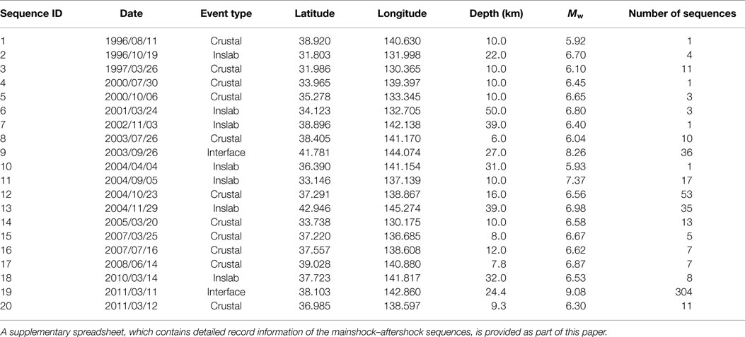
Table 1. Summary of the mainshock characteristics of the 20 mainshock–aftershock sequences.

Figure 1 shows the locations of mainshocks, magnitude–distance plots of mainshocks and major aftershocks, and histogram of V_S30 for the sites included in the database. In the map (Figure 1A), the sequences are divided into four subsets: 2011 Tohoku event (304 sequences), 2003 Tokachi event (36 sequences), crustal events (122 sequences), and interface/inslab events (69 sequences, excluding those for the 2011 Tohoku and 2003 Tokachi events). The magnitudes for the 2011 Tohoku and 2003 Tokachi events are significantly greater than other events (Table 1), whereas the magnitudes for crustal events and interface/inslab events are broadly similar (in the range between M_w6 and M_w7) but their locations are different (i.e., on-shore versus off-shore, indicating different propagation paths). This classification is used for comparing the elastic and inelastic seismic demands of different earthquake types in the following. The magnitude–distance plots indicate that the magnitudes of mainshocks are greater (by approximately one magnitude unit) than those of major aftershocks, which is expected and is broadly consistent with the empirical Bath’s law (Shcherbakov et al., 2005). An implication of these differences is that frequency/spectral content of mainshock records and aftershock records differ significantly (on average). This is important when record scaling is implemented in seismic vulnerability assessment (e.g., incremental dynamic analysis; Goda, 2015). The histogram of V_S30 indicates that the majority of sites included in the developed database are NEHRP site class C or D, and recordings at NEHRP site class A/B or E are rare.

FIGURE 1

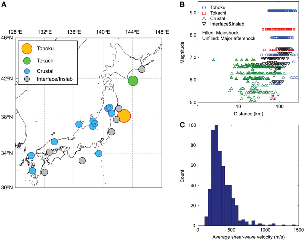
Figure 1. Ground-motion data characteristics: (A) spatial distribution of mainshocks, (B) magnitude–distance plots of mainshocks and major aftershocks, and (C) histogram of average shear-wave velocity in the uppermost 30 m.

Figure 2A compares the statistics (median, 16th percentile, and 84th percentile) of the 5%-damped response spectra that are calculated using the four datasets (i.e., Tohoku, Tokachi, Crustal, and Interface and Inslab). Figure 2B shows the histogram of PGA for the four datasets. Two key observations from Figure 2A are: (i) at short vibration periods (T < 0.5 s), response spectra for the Tohoku dataset are greater than the other three, whereas (ii) at moderate-to-long vibration periods (T > 0.5 s), response spectra for the Tohoku and Tokachi datasets are similar and are significantly greater than those for the Crustal and Interface and Inslab datasets. The seismic intensity parameters (for example, PGA as shown in Figure 2B) vary within the dataset significantly. Although the direct comparisons of the response spectra are not readily applicable due to different record features of these datasets (Figure 1), the former observation can be attributed to the complex source process of the 2011 Tohoku mainshock with high stress drop and low attenuation path (Goda et al., 2013). The latter can be explained by the differences of the earthquake magnitude (i.e., M_w8–9 versus M_w6–7; the source spectra tend to contain richer low-frequency content with increasing magnitude; Stein and Wysession, 2003). The important point is that the damage potential of ground-motion records can be associated with physical features of the source and path effects, and the developed database for MS–AS sequences is useful for investigating the effects of such features on the inelastic seismic demand statistically. This is the main focus of the subsequent sections.

FIGURE 2

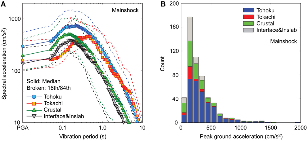
Figure 2. (A) Median, 16th percentile, and 84th percentile of response spectra (mainshocks) and (B) histogram of average PGA (mainshocks).

Bouc–Wen Hysteretic Model

Hysteretic features of structures significantly affect the assessment of non-linear damage potential in a complex way and are important for inelastic seismic demand estimation. The Bouc–Wen model facilitates the flexible hysteresis representation, including degradation and pinching. In normalized displacement space, the equations of motion can be expressed as:

$\begin{array}{llll}\hfill & \ddot{\mu }+\mathrm{2\xi \omega }\ddot{\mathrm{\mu }}+\mathrm{\alpha }{\mathrm{\omega }}_{}^{\text{2}}\mathrm{\mu }+\left(1-\mathrm{\alpha }\right){\mathrm{\omega }}_{}^{\text{2}}{\mathrm{\mu }}_{\text{z}}=-{ü}_{\text{g}}\left(t\right)∕u_{\text{y}}& \hfill & \\ \hfill & {\ddot{\mathrm{\mu }}}_{\text{z}}=\frac{h\left({\mathrm{\mu }}_{\text{z}}\text{,}{\mathrm{\epsilon }}_{\text{n}}\right)}{1+{\mathrm{\delta }}_{\mathrm{\eta }}{\mathrm{\epsilon }}_{\text{n}}}\left[\ddot{\mathrm{\mu }}-\left(1+{\mathrm{\delta }}_{\mathrm{\nu }}{\mathrm{\epsilon }}_{\text{n}}\right)\left(\mathrm{\beta }\left|\ddot{\mathrm{\mu }}\right|{\left|{\mathrm{\mu }}_{\text{z}}\right|}^{\text{n-1}}{\mathrm{\mu }}_{\text{z}}\text{+\hspace{0.17em}}\mathrm{\gamma }\ddot{\mathrm{\mu }}{\left|{\mathrm{\mu }}_{\text{z}}\right|}^{\text{n}}\right)\right]& \hfill & \end{array}$

$\begin{array}{cc}\hfill & h\left({\mathrm{\mu }}_{\text{z}}\text{,}{\mathrm{\epsilon }}_{\text{n}}\right)=1-{\mathrm{\zeta }}_{\text{s}}\left(1-e^{\text{-p}{\mathrm{\epsilon }}_{\text{n}}}\right)\exp \times \left(-{\left(\frac{{\mathrm{\mu }}_{\text{z}}\mathit{sgn}\left(\ddot{\mathrm{\mu }}\right)-q∕{\left[\left(1+{\mathrm{\delta }}_{\mathrm{\nu }}{\mathrm{\epsilon }}_{\text{n}}\right)\left(\mathrm{\beta }+\mathrm{\gamma }\right)\right]}^{\text{1/n}}}{\left(\mathrm{\lambda }\text{+}{\mathrm{\zeta }}_{\text{s}}\left[1-e^{\text{-p}{\mathrm{\epsilon }}_{\text{n}}}\right]\right)\left(\mathrm{\psi }\text{+}{\mathrm{\delta }}_{\mathrm{\psi }}{\mathrm{\epsilon }}_{\text{n}}\right)}\right)}^2\right)\hfill \\ \hfill & {\ddot{\mathrm{\epsilon }}}_{\text{n}}=\left(1-\mathrm{\alpha }\right)\ddot{\mathrm{\mu }}{\mathrm{\mu }}_{\text{z}}\hfill \end{array}$ (1)

where μ and μ_z are the displacement and hysteretic displacement, respectively, normalized by the yield displacement capacity of an inelastic SDOF system u_y (i.e., μ = u/u_y and μ_z = z/u_y, in which u and z are the displacement and hysteretic displacement, respectively); a dot represents the differential operation with respect to time; ξ is the damping ratio; ω is the natural vibration frequency (rad/s); ü_g(t) is the ground acceleration time-history; h(μ_z,ε_n) is the pinching function; ε_n is the normalized hysteresis energy; α, β, γ, and n are the shape parameters; δ_ν and δ_η are the degradation parameters; ζ_s, p, q, ψ, δ_ψ, and λ are the pinching parameters; and sgn(•) is the signum function. The main characteristics of the Bouc–Wen hysteretic systems are defined by the second relationship in Eq. 1, where non-linear restoring force is a function of the imaginary hysteretic displacement. More detailed explanations of the Bouc–Wen parameters can be found in Foliente (1993).

Inelastic seismic demand potential can be quantified using various damage measures. For the case of inelastic SDOF systems, choice of damage measures can be reduced to a few popular ones, such as peak ductility demand and residual ductility demand (Ruiz-García and Miranda, 2003, 2006). The peak ductility demand μ_max is defined as μ_max = max(|μ(t)|) for all t, while the residual ductility demand μ_res is defined as μ_res = μ(t = ∞). For a given ground-motion record, μ_max can be evaluated for a combination of the natural vibration period T (= 2π/ω) and the yield displacement capacity u_y. For convenience, the yield displacement capacity of a system is specified in terms of spectral acceleration at yielding S_ay, rather than spectral displacement at yielding S_dy [i.e., S_ay = S_dy (2π/T)²].

In total, 112 inelastic SDOF systems (combinations of four vibration periods, seven yield strengths, and four hysteresis models) are considered for assessing the non-linear seismic demand parameters (i.e., μ_max and μ_res) subjected to the 531 MS–AS sequences. The intact vibration periods are: T = 0.2, 0.5, 1.0, and 2.0 s (which cover a typical range for the first vibration mode dominated structures). The yield spectral acceleration levels are varied from 0.05 to 1.0 g: S_ay = 0.05, 0.1, 0.15, 0.2, 0.3, 0.5, and 1.0 g, which cover a range of existing structures broadly. For a given set of ground-motion records, systems with larger S_ay values are expected to behave linearly, while systems with smaller S_ay values tend to behave non-linearly. It is also instructive to compare the considered values of S_ay with the response spectra of the record data (Figure 2A). Four hysteretic models are considered: elastic-perfectly plastic (EPP) model (α = 0.0, β = γ = 0.5, n = 25, δ_ν = δ_η = ζ_s = 0.0), smooth bilinear model (α = 0.05, β = γ = 0.5, n = 1, δ_ν = δ_η = ζ_s = 0.0), degrading model without pinching (α = 0.05, β = γ = 0.5, n = 1, δ_ν = 0.1, δ_η = 0.05, ζ_s = 0.0), and degrading model with pinching (α = 0.05, β = γ = 0.5, n = 1, δ_ν = 0.1, δ_η = 0.05, ζ_s = 0.9, p = 2.5, q = 0.15, ψ = 0.1, δ_ψ = 0.005, and λ = 0.5). Figure 3 illustrates normalized displacement μ versus normalized restoring force αμ + (1 − α)μ_z, for the four Bouc–Wen hysteretic models.

FIGURE 3

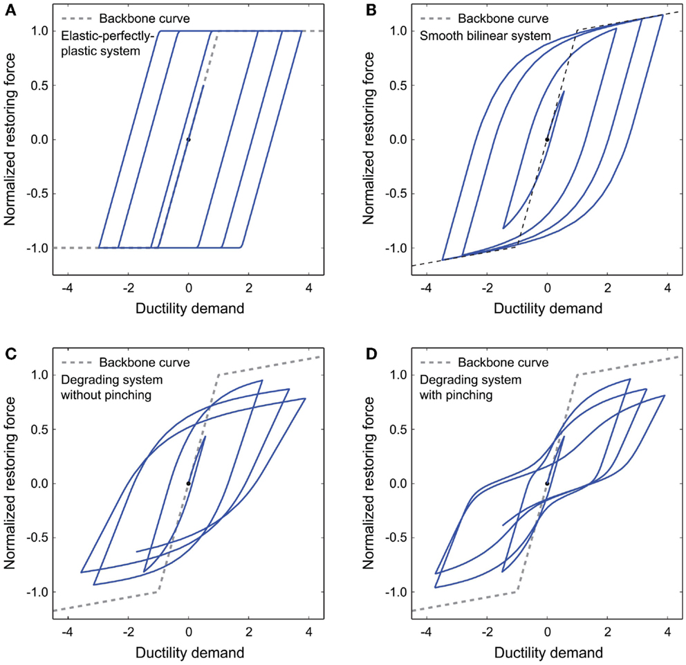
Figure 3. Bouc–Wen hysteretic models: (A) elastic-perfectly plastic system, (B) smooth bilinear system, (C) degrading system, and (D) degrading system with pinching.

Regarding the selected values of S_ay in this study, Nagato and Kawase (2004) estimated seismic capacities of reinforced concrete (RC), steel, and wooden structures using damage statistics from the 1995 Kobe earthquake. The methodology was to calibrate a yield base shear coefficient of an inelastic structural system (i.e., total shear force at base divided by total weight) such that the predicted damage statistics from the set of structural models approximately match actual damage statistics from the 1995 Kobe earthquake. Their results indicate: (i) for RC buildings (3-story to 12-story), natural vibration periods are around 0.3–0.8 s and average yield base shear coefficients are around 0.3–0.7 (depending on the number of stories; generally, low-rise structures have shorter vibration periods and greater base shear coefficients), (ii) for steel buildings (3-story to 5-story), natural vibration periods are around 0.5–0.9 s and average yield base shear coefficients are around 0.4–0.7, and (iii) for wooden buildings (2-story), natural vibration periods are about 0.3 s and average yield base shear coefficients are about 0.4–0.7. The drift ratios corresponding to the yield base shear coefficients are about 0.007–0.01, 0.005–0.008, and 0.01–0.015 for RC, steel, and wooden structures, respectively. It is noteworthy that the definition of the yield capacity point depends on the specifics of the adopted structural models; for instance, Nagato and Kawase (2004) used a trilinear force-deformation curve to characterize the hysteretic behavior. If a bilinear representation is considered, instead of the trilinear one, the yield point typically is located somewhere between the first and second yield points of the trilinear curve. Moreover, the calibrated structural models should be only regarded as representative, whereas actual structures have significant variability/uncertainty with regard to their yield (and ultimate) capacities; according to Nagato and Kawase (2004), factors of 0.5 and 2.0 are possible. Based on the above information, it is thus possible to associate the inelastic SDOF systems that are considered in this study with typical buildings in Japan.

Non-Linear Seismic Demand Assessment

The main objectives of this section are: (i) to investigate the effects of earthquake types, magnitudes, and hysteretic behavior on the peak and residual ductility demands and (ii) to evaluate the effects of major aftershocks on the non-linear structural responses. In addition, spatial aspect of the aftershock effects is evaluated for the 2011 Tohoku sequences. In the following, MS–AS sequences having V_S30 between 150 and 600 m/s (most prevalent site conditions in Japan) are focused upon (see Figure 1C); the total number of MS–AS sequences is 492. Initially, EPP models are used as base case and later other hysteretic models are considered (Figure 3). In the following, the discussion is focused upon structural systems having vibration periods of 0.2 and 1.0 s due to limitations of space. The results obtained for these two periods can be interpolated/extrapolated to structural systems with vibration periods of 0.5 and 2.0 s by taking into account input ground motion and structural characteristics. The detailed results for systems that are not presented in detail are available upon request.

Effects of Earthquake Types

First, subsets of the entire MS–AS database are focused upon to examine the similarity or dissimilarity of the non-linear seismic demand potential for different earthquake types. They are obtained by limiting sequences having the average PGA between 100 and 200 cm/s² (see Figure 2B). This criterion is selected such that homogenous datasets (to the extent possible) can be obtained for the Tohoku, Tokachi, Crustal, and Interface and Inslab events. The number of sequences is 69, 21, 38, and 36 for the Tohoku, Tokachi, Crustal, and Interface and Inslab subsets, respectively. These are considered as sufficient to obtain the statistics of the structural responses, noting that each sequence consists of two horizontal components. Figure 4A compares the median, 16th percentile, and 84th percentile of the response spectra for the four datasets. The result indicates that the response spectra for the Tohoku and Tokachi subsets are similar in terms of median and 16th/84th percentiles (i.e., red versus blue); the same can be observed for the Crustal and Interface and Inslab subsets (i.e., green versus black). On the other hand, the response spectra for the Tohoku and Tokachi subsets are significantly different from those for the Crustal and Interface and Inslab subsets (i.e., red/blue versus green/black). The main reason for the different elastic response spectra is the earthquake magnitude. It is noted that the differences of the response spectra in the short-period range for the Tohoku and Tokachi datasets that are observed in Figure 2A (by considering the entire database) disappear when more homogeneous datasets are considered.

FIGURE 4

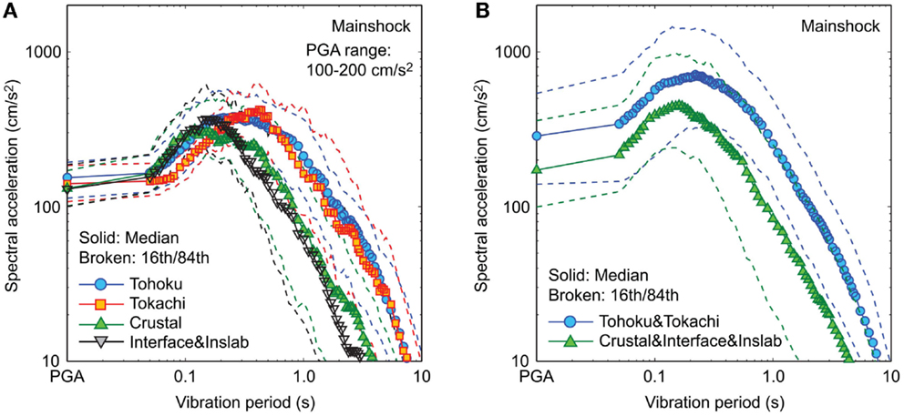
Figure 4. Comparison of median, 16th percentile, and 84th percentile of response spectra (mainshocks): (A) Tohoku, Tokachi, Crustal, and Interface and Inslab datasets having average PGA between 100 and 200 cm/s² and (B) Tohoku and Tokachi and Crustal, Interface, and Inslab datasets.

Figure 5 shows the cumulative probability distributions of the peak and residual ductility demands of two EPP models with T = 0.2 s and S_ay = 0.2 g and with T = 1.0 s and S_ay = 0.1 g due to mainshock records only by considering the four subsets having the average PGA between 100 and 200 cm/s². The two systems are selected to illustrate the interesting results clearly and concisely (among many cases), and they correspond to structures with low seismic capacities among the existing building stock in Japan. The results shown in Figure 5 indicate that both peak and residual ductility demands for the Tohoku and Tokachi subsets are greater than those for the Crustal and Interface and Inslab datasets. The differences of the non-linear structural responses are greater for T = 1.0 s and for residual ductility demands. The differences can be attributed to the response spectral characteristics of these subsets, shown in Figure 4A. Another attribute that has influence on residual ductility demand is the duration. The seismological source parameter that affects the spectral content and duration of ground motions is the earthquake magnitude.

FIGURE 5

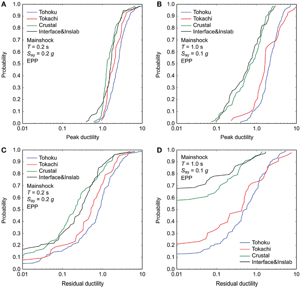
Figure 5. Comparison of cumulative probability plots of ductility demands of EPP models due to mainshock records only by considering four subsets having average PGA between 100 and 200 cm/s²: (A) peak ductility demand for T = 0.2 s and S_ay = 0.2 g, (B) peak ductility demand for T = 1.0 s and S_ay = 0.1 g, (C) residual ductility demand for T = 0.2 s and S_ay = 0.2 g, and (D) residual ductility demand for T = 1.0 s and S_ay = 0.1 g.

To cover the parameter space of the calculated cases more widely, peak as well as residual ductility demand curves for EPP models (T = 0.2 and 1.0 s) with different yield spectral accelerations are compared in Figure 6 by considering the four subsets. The peak ductility demand curves gradually decrease with increasing yield spectral acceleration (i.e., stronger systems), whereas the slopes of the residual ductility demand curves are steeper than those of the peak ductility demand curves. These suggest that for the considered EPP models, seismic damage due to transient peak demands can occur for relatively moderate ground motions, whereas seismic damage due to permanent residual demands occurs when severe ground motions affect the structures. Importantly, the results confirm the similarity of peak and residual ductility demands for the Tohoku and Tokachi datasets and for the Crustal and Interface and Inslab datasets, and that the former is greater than the latter. The conclusions are applicable to different hysteretic models as well as subsets with different selection criteria.

FIGURE 6

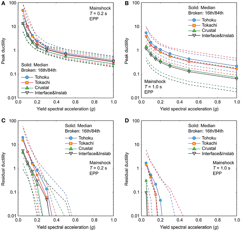
Figure 6. Comparison of ductility demand curves for EPP models with different yield spectral accelerations due to mainshock records only by considering four subsets having average PGA between 100 and 200 cm/s²: (A) peak ductility demand for T = 0.2 s, (B) peak ductility demand for T = 1.0 s, (C) residual ductility demand for T = 0.2 s, and (D) residual ductility demand for T = 1.0 s.

Effects of Magnitudes and Hysteretic Behavior

Based on the above results, one of the controlling features of the ductility demands is the earthquake magnitude. To further investigate the key features that affect the non-linear seismic demand potential (i.e., hysteretic characteristics and major aftershocks), the entire MS–AS dataset is divided into two subsets according to the magnitude ranges: the Tohoku and Tokachi (T&T), or large-magnitude, dataset (319 sequences) and the Crustal, Interface, and Inslab (C&I&I), or moderate-magnitude, dataset (173 sequences). Figure 4B compares the median, 16th percentile, and 84th percentile of the response spectra for the two datasets. The response spectra for the large-magnitude dataset are greater than those for the moderate-magnitude dataset. The response spectral shape for the former dataset has richer long-period spectral content, in comparison with that for the latter dataset.

To inspect the results for specific systems, data points of peak/residual ductility demands and corresponding spectral acceleration values at the intact vibration periods are plotted in Figure 7. The considered systems are two EPP models with T = 0.2 s and S_ay = 0.2 g and with T = 1.0 s and S_ay = 0.1 g subjected to MS–AS sequences. In the figure, individual data points are displayed with small markers, whereas larger markers with a line show the median trend of the individual data. In the context of the PBEE methodology, ductility demands are the engineering demand parameters (EDP) and spectral accelerations are the intensity measures (IM). The results shown in Figure 7 are the assessments of inelastic seismic demand (i.e., empirical IM–EDP relationships) based on cloud analysis (Jalayer and Cornell, 2009). Note that the main objective of this study is not the development of the (generic) inelastic seismic demand prediction models (e.g., constant R approach). Rather, it is focused upon identifying the key factors that result in different inelastic seismic demand predictions, and thus these parameters should be incorporated in developing such prediction models for specific structures.

FIGURE 7

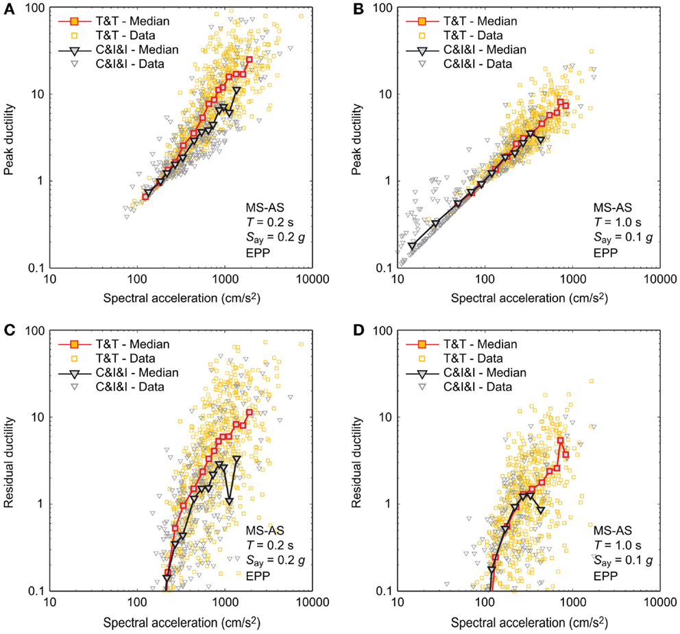
Figure 7. Ductility demand – spectral acceleration curves for EPP models due to MS–AS sequences by considering the Tohoku and Tokachi (T&T) dataset and the Crustal, Interface, and Inslab (C&I&I) dataset: (A) peak ductility demand for T = 0.2 s and S_ay = 0.2 g, (B) peak ductility demand for T = 1.0 s and S_ay = 0.1 g, (C) residual ductility demand for T = 0.2 s and S_ay = 0.2 g, and (D) residual ductility demand for T = 1.0 s and S_ay = 0.1 g.

A notable trend of the results shown in Figure 7 related to the magnitude ranges of the ground-motion data is that for T = 0.2 s (Figures 7A,C), the median ductility demand curves (both peak and residual) for the large-magnitude dataset are greater than those for the moderate-magnitude dataset. On the other hand, such differences are not observed for T = 1.0 s (Figures 7B,D). This may appear to be inconsistent with the results shown in Figures 5 and 6. The different trends are caused because in Figure 7, the base parameters for describing the seismic hazard intensity (i.e., IM) are the spectral accelerations at the intact vibration periods, while in Figures 5 and 6, the base IM parameter is the PGA (note: PGA is a popular parameter for record selection purposes). For the considered systems, spectral accelerations at the intact vibration period are more efficient than PGA (i.e., an IM–EDP relationship is characterized by smaller variability of the relationship; Luco and Cornell, 2007), and it is customary to adopt more efficient IMs in evaluating the values of EDP (however, full exploration of efficient IMs is beyond the scope of this study). More specifically, when the response spectra of the large-magnitude dataset and of the moderate-magnitude dataset are matched at T = 0.2 s (see Figure 4B), the former has the richer spectral content than the latter in the vibration period range greater than T = 0.2 s and when the structural systems go into the inelastic response domain, inelastic responses of the systems are strongly affected by ground motions in the vibration period range longer than the intact vibration period (Luco and Bazzurro, 2007). When the matching of response spectra is carried out at T = 1.0 s, the matched response spectra in the vibration period range longer than 1.0 s become similar (note: in this case, major differences appear in the vibration period range shorter than 1.0 s; however, the inelastic SDOF systems considered in this study are not sensitive to ground motions in this period range). Further to note, although no results are presented and discussed in this study, results for inelastic seismic demand estimation based on the constant R approach using the same MS–AS sequence datasets indicate that the magnitude effects on the ductility demands are significant for short-period structures.

Returning to the original focus of this study (i.e., empirical assessment of ductility demands), Figure 8 compares peak ductility demand curves for EPP models subjected to MS–AS sequences with those for smooth bilinear models, degrading models, and degrading models with pinching (Figure 3). Both large- and moderate-magnitude datasets are considered. The intension of this figure is to present the effects of hysteretic characteristics of the inelastic SDOF systems on the peak ductility demands; it is not to compare the peak ductility demands for the two datasets (which is not of interest because the seismic excitation levels are different). In these comparisons, EPP systems are used as reference and thus their results are shown in all figure panels.

FIGURE 8

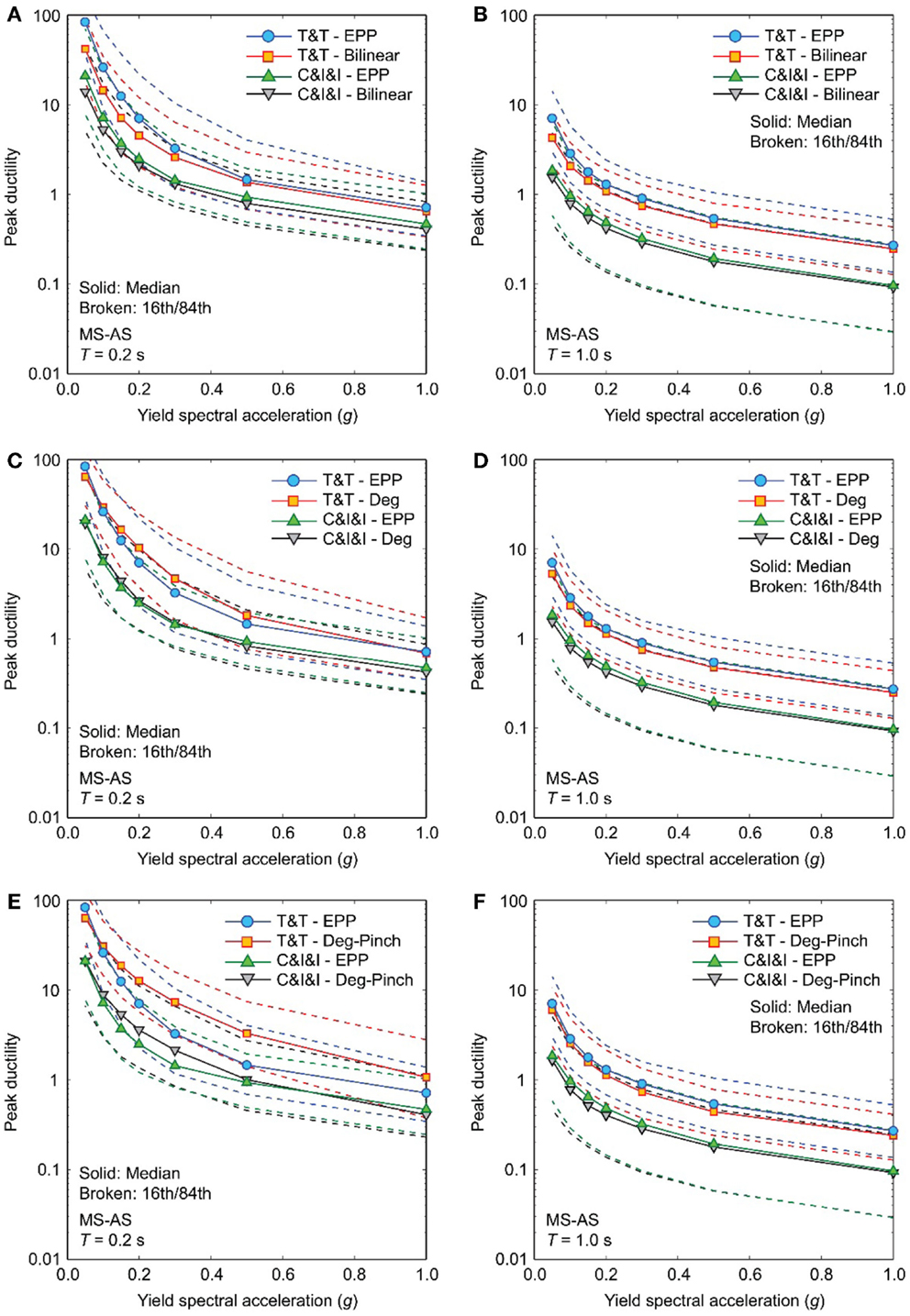
Figure 8. Comparison of peak ductility demand curves for different hysteretic models with different yield spectral accelerations due to MS–AS sequences by considering the Tohoku and Tokachi (T&T) dataset and the Crustal, Interface, and Inslab (C&I&I) dataset: (A,B) bilinear models for T = 0.2 and 1.0 s, (C,D) degrading models for T = 0.2 and 1.0 s, and (E,F) degrading models with pinching for T = 0.2 and 1.0 s.

Figures 8A,B suggest that the consideration of smooth bilinear systems (α and n are changed from EPP systems) leads to the decreased peak ductility demand, and that the extent of reduction of the peak ductility demand is greater for T = 0.2 s than for T = 1.0 s. The key factor for the decreased peak ductility demand is α (Ma et al., 2004). The consideration of degrading effects (Figures 8C,D) results in the increased peak ductility demand. The influence of degradation is more significant for T = 0.2 s than T = 1.0 s. For T = 0.2 s, the peak ductility demand curves for the degrading systems become greater than those for the EPP systems (i.e., overcoming the reduction due to the positive post-yield stiffness ratio), whereas for T = 1.0 s, the increase is minimal. The pinching behavior affects the structural systems having short vibration periods, whereas its effect on systems with long vibration periods is not significant (Figures 8E,F). For T = 0.2 s, the effect due to pinching behavior is particularly large, increasing the peak ductility demands in the low-to-moderate ranges significantly. It is noted that the effects of hysteretic behavior, as demonstrated above, depend on the vibration period as well as seismic excitation level. The above-mentioned observations are in agreement with Goda and Atkinson (2009).

The similar comparisons for the residual ductility demands for different hysteretic models are omitted for brevity. It is observed that when the hysteretic behavior is changed from EPP systems to other systems having positive post-yield stiffness ratios (i.e., α = 0.0 versus α = 0.05), the absolute values of the residual ductility demand decrease dramatically. For instance, the overall trends of the residual ductility demand curves for the EPP systems (T = 0.2 and 1.0 s) by considering the large-magnitude and moderate-magnitude datasets are similar to those shown in Figure 6. When the bilinear and degrading systems without/with pinching are considered, the absolute values of the residual ductility demand curves become significantly less (median as well as 84th percentile curves rarely exceed the ductility demand of 0.1, which is of no engineering significance). These results are in agreement with Ruiz-García and Miranda (2006).

Effects of Major Aftershocks

The effects of major aftershocks on the peak and residual ductility demands are evaluated by considering the large- and moderate-magnitude datasets. To inspect the impact of major aftershocks visually, median, 84th percentile, and 98th percentile of the MS–AS to mainshock ductility demand ratios (i.e., MS–AS to MS ratios) for EPP models (T = 0.2 and 1.0 s) are presented in Figure 9. Because the MS–AS to MS ratios can be extremely large when ductility demands for mainshock records only are small (this is particularly applicable to residual ductility demands) and such cases are of little engineering interests, the MS–AS to MS ratios are computed using peak/residual ductility demands due to mainshocks greater than 0.1. Figure 9 shows that for the majority of the cases, the median ratios are 1 (both peak and residual), indicating that more than 50% of the cases, the major aftershocks do not increase the seismic demand levels caused by the mainshocks. However, in rare cases, the major aftershocks can increase the seismic damage extent significantly. The extent of the aftershock effects is greater for the moderate-magnitude dataset than for the large-magnitude dataset. For instance, the 98th percentile curves of the MS–AS to MS peak ductility demand ratios for the moderate- and large-magnitude datasets range around 2–3 and 1.5–2, respectively. The comparison of the results for the peak and residual ductility demands indicates that the MS–AS to MS ratios for the residual ductility demands are more sensitive than those for the peak ductility demands; these are partly attributed to the fact that for EPP systems the absolute values of the residual ductility demands are smaller than those of the peak ductility demands and the residual ductility demands tend to increase more rapidly with the yield spectral acceleration (Figure 6).

FIGURE 9

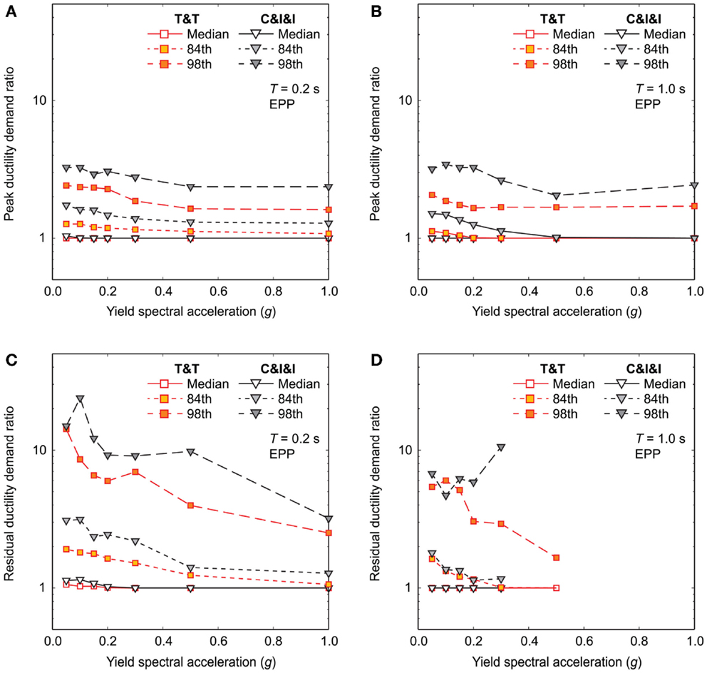
Figure 9. Statistics of the MS–AS to mainshock ductility demand ratios for EPP models by considering the Tohoku and Tokachi (T&T) dataset and the Crustal, Interface, and Inslab (C&I&I) dataset: (A) peak ductility demand for T = 0.2 s, (B) peak ductility demand for T = 1.0 s, (C) residual ductility demand for T = 0.2 s, and (D) residual ductility demand for T = 1.0 s.

To further investigate the aftershock effects in terms of hysteretic behavior, Figure 10 compares the 84th percentile and 98th percentile curves of the MS–AS to MS peak ductility demand ratios for different hysteretic models (note: 50th percentile curves are not shown as they are equal to 1 for most of the cases). Both large- and moderate-magnitude datasets are considered. Similarly to Figure 8, the results for EPP systems are used as reference. The consideration of bilinear systems with positive post-yield stiffness ratios results in slightly smaller MS–AS to MS peak ductility demand ratios (e.g., 84th percentile curves for T = 0.2 s), however, the overall impact is not significant (Figures 10A,B). The results for the degrading systems without/with pinching indicate that the MS–AS to MS peak ductility demand ratios for T = 0.2 s are slightly more influenced by hysteretic behavior than the ratios for T = 1.0 s (Figures 10C–F). Noticeable increases of the MS–AS to MS ratios are observed due to pinching behavior for T = 0.2 s (Figure 10E). Overall, it can be concluded that the effects of hysteretic characteristics on the MS–AS to MS peak ductility demand ratios are not particularly large. The similar results for the MS–AS to MS residual ductility demand ratios are omitted because the residual ductility demands for bilinear and degrading systems without/with pinching are small (the majority of the data are below the threshold of 0.1).

FIGURE 10

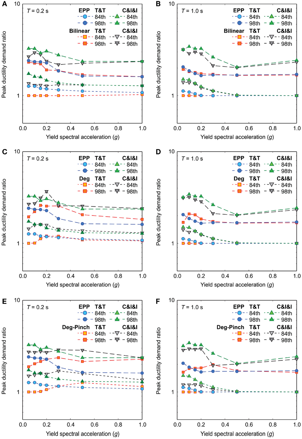
Figure 10. Statistics of MS–AS to mainshock peak ductility demand ratios for different hysteretic models by considering the Tohoku and Tokachi (T&T) dataset and the Crustal, Interface, and Inslab (C&I&I) dataset: (A,B) bilinear models for T = 0.2 and 1.0 s, (C,D) degrading models for T = 0.2 and 1.0 s, and (E,F) degrading models with pinching for T = 0.2 and 1.0 s.

Finally, dependency of the MS–AS to MS ratios (both peak and residual) of EPP systems on various seismological parameters is investigated using the large- and moderate-magnitude datasets. The considered explanatory parameters are: mainshock peak/residual ductility demand, average shear-wave velocity (V_S30), mainshock magnitude, mainshock distance, aftershock magnitude, aftershock distance, mainshock PGA, mainshock spectral acceleration at the intact vibration period, aftershock PGA, and aftershock spectral acceleration at the intact vibration period. By visually inspecting the scatter plots of the MS–AS to MS ratios with respect to the examined parameters and by carrying out linear regression analysis (note: regression analyses are performed in log–log space, except for the mainshock/aftershock magnitude), their dependency is evaluated. The dependency between the MS–AS to MS ratios and the parameters is judged to be significant when the 95% confidence intervals of the slope coefficient do not include zero (i.e., confidence intervals are either both positive or both negative). The regression analysis results suggest that the MS–AS to MS peak ductility demand ratios clearly depend on aftershock PGA and spectral acceleration at the intact vibration period, while they are weakly dependent on the mainshock peak ductility demand. The former is simply interpreted that stronger aftershocks have greater potential to cause additional seismic damage, whereas the latter can be understood that relative effects due to major aftershocks become less critical when the mainshock causes large seismic damage to structures. Note that minor trends can be recognized for aftershock magnitude and distance; however, the trends are not consistent for the majority of cases and these parameters are regarded as secondary factors that affect aftershock PGA and spectral accelerations. On the other hand, the results for the MS–AS to MS residual ductility demand ratios are less clear because of large scatter of the data points. Therefore, it is concluded that the dependency between the MS–AS to MS residual ductility demand ratios and the aftershock elastic response parameters is too weak. To illustrate the above-mentioned observations, Figure 11 presents the scatter plots of the MS–AS to MS ratio and the aftershock PGA for EPP systems with T = 0.2 s and S_ay = 0.2 g and with T = 1.0 s and S_ay = 0.1 g by considering the large- and moderate-magnitude datasets. In the figure panels, the regression lines as well as the slope value and its confidence intervals are included. For the peak ductility demands, clear positive trends are observed for T = 0.2 s, whereas such trends become weak for T = 1.0 s. Generally, aftershock spectral accelerations at the intact vibration period are more correlated with the MS–AS to MS ratios. Figure 11 also shows that the scatter of the data points for the residual ductility demands is significantly greater than that for the peak ductility demands.

FIGURE 11

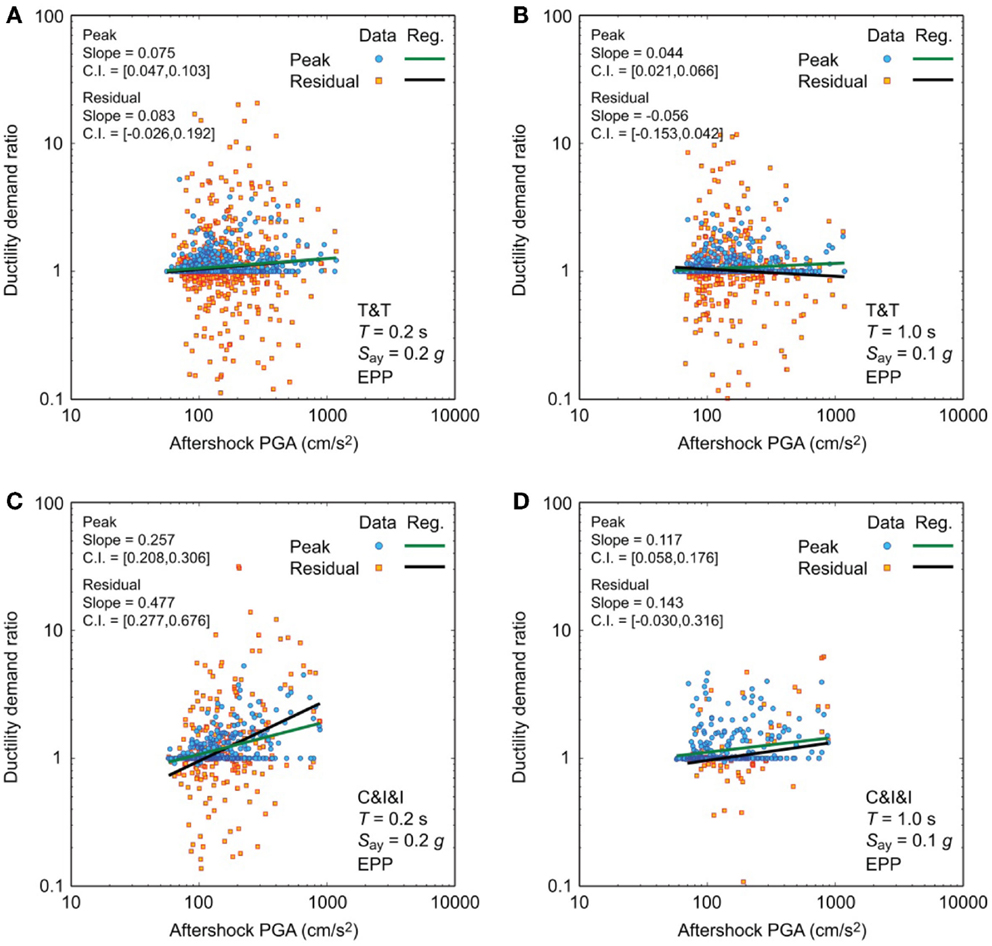
Figure 11. Dependency of MS–AS to mainshock peak and residual ductility demand ratios for EPP systems by considering: (A) Tohoku and Tokachi (T&T) dataset for T = 0.2 s and S_ay = 0.2 g, (B) Tohoku and Tokachi (T&T) dataset for T = 1.0 s and S_ay = 0.1 g, (C) Crustal, Interface, and Inslab (C&I&I) dataset for T = 0.2 s and S_ay = 0.2 g, and (D) Crustal, Interface, and Inslab (C&I&I) dataset for T = 1.0 s and S_ay = 0.1 g.

Spatial Distribution of Major Aftershocks for the 2011 Tohoku Sequence

Figure 12 shows the spatial distribution of the peak ductility demands, peak ductility demand ratios, residual ductility demands, and residual ductility demand ratios for two EPP systems with T = 0.2 s and S_ay = 0.2 g and with T = 1.0 s and S_ay = 0.1 g. The intensity of the ductility demands and the ductility demand ratios are color-coded (see the captions in Figure 12); the ranges of the demand values and ratios are chosen to represent different seismic damage severities (e.g., peak ductility demand of 10 is considered to be major damage). In the figure panels for the peak/residual ductility demands (Figures 12A,C,E,G), strong-motion generation areas, which are characterized as areas with large slip velocities within a total rupture plane, are indicated. These areas are estimated by Kurahashi and Iikura (2013) via strong-motion source inversion of the 2011 Tohoku mainshock data. Whereas in the figure panels for the peak/residual ductility demand ratios (Figures 12B,D,F,H), locations of the major aftershocks for the 2011 Tohoku sequences are shown.

FIGURE 12

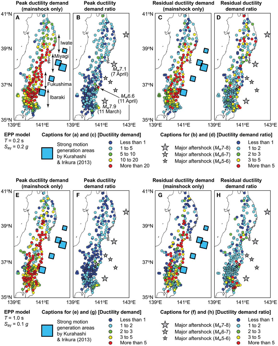
Figure 12. Spatial distribution of ductility demands and ductility demand ratios by considering the Tohoku dataset: (A–D) peak ductility demand, peak ductility demand ratio, residual ductility demand, and residual ductility demand ratio for EPP systems (T = 0.2 s and S_ay = 0.2 g), and (E–H) peak ductility demand, peak ductility demand ratio, residual ductility demand, and residual ductility demand ratio for EPP systems (T = 1.0 s and S_ay = 0.1 g).

Inspection of the results for the peak ductility demands of EPP systems having T = 0.2 s and S_ay = 0.2 g (Figure 12A) indicates that the seismic damage potential due to the mainshock is high at sites around 38–39°N (Miyagi Prefecture) and at sites around 36–37°N (Fukushima and Ibaraki Prefectures). The sites in Miyagi Prefecture are affected by the two overlapping strong-motion generation areas (which resulted in noticeable multiple-shock features of the recorded ground motions), whereas the sites in Fukushima and Ibaraki Prefectures are influenced by the southernmost strong-motion generation area, which is located near the coastline. Furthermore, many of these structures are located along the coast, and therefore are likely to be subjected to the tsunami actions between mainshock and aftershock. Such actions may further degrade the structural behavior and make the buildings weaker, being unable to resist the next seismic excitation. Moreover, it can be observed from Figure 12B that the additional seismic damage occurs in the vicinity of major aftershocks. In particular, the M_w7.9 aftershock off Ibaraki Prefecture that occurred 30 min after the mainshock increases the peak ductility demands at sites in the southern part of Ibaraki Prefecture (green-to-yellow circles in Figure 12B). The M_w7.1 aftershock that occurred on 7 April off Miyagi Prefecture causes small-to-moderate increase of the peak seismic demands in Miyagi Prefecture (light-blue-to-green circles in Figure 12B). Notably, the M_w6.6 aftershock that occurred on 11 April in the upper crust causes a major increase of the peak seismic demands at a nearby location (red circle in Figure 12B). The causal relationship between major aftershocks and increased seismic demands can be understood physically and intuitively; simply, when a major aftershock strikes near a site of interest, the seismic demand potential due to the aftershock becomes greater. The above explanations are applicable to the residual ductility demands (Figures 12C,D) as well as the results for the other EPP system (Figures 12E–H). The results shown in Figure 12 are consistent with the results shown in Figure 11.

From seismic risk-management perspectives, critical situations arise when moderate-to-severe damage is caused by a mainshock and major aftershocks occur nearby, aggravating the conditions of the mainshock-damaged structures. The results shown in Figure 12 highlight that the spatial occurrence process of aftershocks is important. This is a major source of uncertainty in ensuring the safe evacuation and deciding upon the reoccupation of buildings in a post-disaster environment. Moreover, by reflecting upon the observations made regarding Figure 9 (i.e., aftershock effects for the moderate-magnitude dataset is greater than those for the large-magnitude dataset), the reason for less frequent occurrence of damaging aftershocks for mega-thrust subduction earthquakes may be attributed to the fact that mainshock seismic damage is caused at many locations over a larger geographical region but aftershock-triggered seismic damage is concentrated at more local areas. To study such aspects, spatial modeling of aftershock occurrence needs to be incorporated in generating artificial MS–AS sequences (Goda, 2012).

Conclusion

This study aimed at evaluating the peak and residual ductility demands of inelastic SDOF systems due to real MS–AS sequences from an empirical perspective. For this purpose, an extensive dataset of as-recorded MS–AS sequences for Japanese earthquakes was developed (containing 531 sequences; each with two horizontal components). The constructed dataset is large, compared with previous datasets of similar kinds, and thus more rigorous investigations regarding the non-linear seismic demand potential for MS–AS sequences can be carried out. To draw generic conclusions, numerous inelastic SDOF systems having different vibration periods, yield strengths, and hysteretic characteristics that are represented by the Bouc–Wen model, were considered. Such assessment is useful in two aspects. Firstly, it serves as a benchmark, when non-linear structural responses due to large mainshocks having different record characteristics and due to major aftershocks are evaluated using artificial MS–AS data. Back-to-back applications of (scaled) mainshock records as aftershocks often lead to overestimation of the aftershock seismic demand potential (Goda, 2015), and thus careful construction of artificial MS–AS sequences is important. Secondly, investigations of the relationships between seismic demands of inelastic SDOF systems and key seismological parameters of MS–AS sequences provide useful guidance as to which parameters should be taken into account in developing seismic demand prediction models for more realistic structural models. Moreover, the developed MS–AS sequence dataset facilitates the assessment of the aftershock effects in relation to the spatial distribution of major aftershocks. Numerical analysis was set up to investigate the above-mentioned problems.

Based on the analysis results, the following conclusions can be drawn:

1. One of the controlling factors for determining the severity of peak and residual ductility demands (for the same level of seismic excitation) is earthquake magnitude. For inelastic seismic demand estimation, earthquake magnitude or a surrogate measure, such as earthquake event type, may need to be included (depending on regional seismic hazard characteristics).

2. Hysteretic behavior of structural systems can have major influence on the estimation of the inelastic seismic demand. The consideration of the positive post-yield stiffness ratio, in comparison with zero post-yield stiffness ratio as in EPP systems, reduces peak and residual ductility demands (particularly significant impact on the residual ductility demand). Moreover, both degradation and pinching behavior have moderate effects on the peak ductility demand.

3. The aggravation of the inelastic seismic demand due to major aftershocks is not common, because the mainshock often causes severer damage to structures. However, in rare cases, major aftershocks can increase the seismic damage severity significantly. Moreover, hysteretic behavior does not affect the MS–AS to MS peak ductility demand ratios significantly. The key factors for damaging aftershocks are: the ground-motion intensity of major aftershocks and the severity of damage caused by the mainshock.

4. The causal relationship between major aftershocks and increased seismic demands can be understood physically; greater seismic demand potential results in greater seismic demand. For mega-thrust subduction events, such as the 2011 Tohoku earthquake, spatial occurrence process of aftershocks is critical, because the size of major aftershocks is significantly smaller than the mainshock and thus their impact are much more localized. Improved spatial modeling of major aftershocks needs to be incorporated in generating artificial MS–AS sequences for seismic vulnerability assessment.

Conflict of Interest Statement

The authors declare that the research was conducted in the absence of any commercial or financial relationships that could be construed as a potential conflict of interest.

Acknowledgments

Strong-motion data used in this study were obtained from the K-NET and KiK-net (http://www.kyoshin.bosai.go.jp/) and the SK-net (http://www.sknet.eri.u-tokyo.ac.jp/). KG is supported by the Alexander von Humboldt Fellowship for Experienced Researchers. RR is funded by the Engineering and Physical Sciences Research Council (EP/M001067/1).

Supplementary Material

The Supplementary Material for this article can be found online at https://www.frontiersin.org/article/10.3389/fbuil.2015.00006/abstract

Footnotes

1. ^http://www.kyoshin.bosai.go.jp/
2. ^http://www.sknet.eri.u-tokyo.ac.jp/
3. ^http://www.globalcmt.org/
4. ^http://www.fnet.bosai.go.jp/
5. ^http://www.gsi.go.jp/bousai.html
6. ^http://www.eri.u-tokyo.ac.jp/sanchu/Seismo_Note/
7. ^http://www.seis.nagoya-u.ac.jp/sanchu/Seismo_Note/

References

Boore, D. M. (2005). On pads and filters: processing strong-motion data. Bull. Seismol. Soc. Am. 95, 745–750. doi: 10.1785/0120040160

CrossRef Full Text | Google Scholar

Cornell, C. A., Jalayer, F., Hamburger, R. O., and Foutch, D. A. (2002). Probabilistic basis for 2000 SAC Federal Emergency Management Agency steel moment frame guidelines. J. Struct. Eng. 128, 526–533. doi:10.1061/(ASCE)0733-9445(2002)128:4(526)

CrossRef Full Text | Google Scholar

Federal Emergency Management Agency. (2005). Improvement of Nonlinear Static Seismic Analysis Procedures. Washington, DC: Federal Emergency Management Agency.

Google Scholar

Foliente, G. C. (1993). Stochastic Dynamic Response of Wood Structural Systems. Ph.D. dissertation, Virginia Polytechnic Institute and State University, Blacksburg, VA.

Google Scholar

Galasso, C., Zarain, F., Iervolino, I., and Graves, R. W. (2012). Validation of ground motion simulations for historical events using SDOF systems. Bull. Seismol. Soc. Am. 102, 2727–2740. doi:10.1785/0120120018

CrossRef Full Text | Google Scholar

Goda, K. (2012). Nonlinear response potential of mainshock-aftershock sequences from Japanese earthquakes. Bull. Seismol. Soc. Am. 102, 2139–2156. doi:10.1785/0120110329

CrossRef Full Text | Google Scholar

Goda, K. (2015). Record selection for aftershock incremental dynamic analysis. Earthquake Eng. Struct. Dyn. 44, 1157–1162. doi:10.1002/eqe.2513

CrossRef Full Text | Google Scholar

Goda, K., and Atkinson, G. M. (2009). Seismic demand estimation of inelastic SDOF systems for earthquakes in Japan. Bull. Seismol. Soc. Am. 99, 3284–3299. doi:10.1785/0120090107

CrossRef Full Text | Google Scholar

Goda, K., and Atkinson, G. M. (2010). Intraevent spatial correlation of ground-motion parameters using SK-net data. Bull. Seismol. Soc. Am. 100, 3055–3067. doi:10.1785/0120100031

CrossRef Full Text | Google Scholar

Goda, K., Pomonis, A., Chian, S. C., Offord, M., Saito, K., Sammonds, P., et al. (2013). Ground motion characteristics and shaking damage of the 11th March 2011 M_w9.0 Great East Japan earthquake. Bull. Earthquake Eng. 11, 141–170. doi:10.1007/s10518-012-9371-x

CrossRef Full Text | Google Scholar

Goulet, C. A., Haselton, C. B., Mitrani-Reiser, J., Beck, J. L., Deierlein, G. G., Porter, K. A., et al. (2007). Evaluation of the seismic performance of a code-conforming reinforced-concrete frame building – from seismic hazard to collapse safety and economic losses. Earthquake Eng. Struct. Dyn. 36, 1973–1997. doi:10.1002/eqe.694

CrossRef Full Text | Google Scholar

Iervolino, I., and Cornell, C. A. (2005). Record selection for nonlinear seismic analysis of structures. Earthquake Spectra 21, 685–713. doi:10.1193/1.1990199

CrossRef Full Text | Google Scholar

Jalayer, F., and Cornell, C. A. (2009). Alternative nonlinear demand estimation methods for probability-based seismic assessments. Earthquake Eng. Struct. Dyn. 38, 951–972. doi:10.1002/eqe.876

CrossRef Full Text | Google Scholar

Kagan, Y. Y. (2002). Aftershock zone scaling. Bull. Seismol. Soc. Am. 92, 641–655. doi:10.1785/0120010172

CrossRef Full Text | Google Scholar

Kurahashi, S., and Iikura, K. (2013). Short-period source model of the 2011 M_w 9.0 off the Pacific coast of Tohoku earthquake. Bull. Seismol. Soc. Am. 103, 1373–1393. doi:10.1785/0120120157

CrossRef Full Text | Google Scholar

Li, Q., and Ellingwood, B. R. (2007). Performance evaluation and damage assessment of steel frame buildings under main shock-aftershock earthquake sequences. Earthquake Eng. Struct. Dyn. 36, 405–427. doi:10.1002/eqe.667

CrossRef Full Text | Google Scholar

Luco, N., and Bazzurro, P. (2007). Does amplitude scaling of ground motion records result in biased nonlinear structural drift responses? Earthquake Eng. Struct. Dyn. 36, 1813–1835. doi:10.1002/eqe.695

CrossRef Full Text | Google Scholar

Luco, N., and Cornell, C. A. (2007). Structure-specific scalar intensity measures for near-source and ordinary earthquake ground motions. Earthquake Spectra 23, 357–392. doi:10.1193/1.2723158

CrossRef Full Text | Google Scholar

Ma, F., Zhang, H., Bockstedte, A., Foliente, G. C., and Paevere, P. (2004). Parameter analysis of the differential model of hysteresis. ASME J. Appl. Mech. 71, 342–349. doi:10.1115/1.1668082

CrossRef Full Text | Google Scholar

Morikawa, N., and Fujiwara, H. (2013). A new ground motion prediction equation for Japan applicable up to M9 mega-earthquake. J. Disaster Res. 8, 878–888.

Google Scholar

Moustafa, A., and Takewaki, I. (2010). Modeling critical ground-motion sequences for inelastic structures. J. Adv. Struct. Eng. 13, 665–680. doi:10.1260/1369-4332.13.4.665

CrossRef Full Text | Google Scholar

Nagato, K., and Kawase, H. (2004). Damage evaluation models of reinforced concrete buildings based on the damage statistics and simulated strong motions during the 1995 Hyogo-ken Nanbu earthquake. Earthquake Eng. Struct. Dyn. 33, 755–774. doi:10.1002/eqe.376

CrossRef Full Text | Google Scholar

Ramirez, C. M., and Miranda, E. (2012). Significance of residual drifts in building earthquake loss estimation. Earthquake Eng. Struct. Dyn. 41, 1477–1493. doi:10.1002/eqe.2217

CrossRef Full Text | Google Scholar

Ruiz-García, J. (2012). Mainshock-aftershock ground motion features and their influence in building’s seismic response. J. Earthquake Eng. 16, 719–737. doi:10.1080/13632469.2012.663154

CrossRef Full Text | Google Scholar

Ruiz-García, J., and Miranda, E. (2003). Inelastic displacement ratios for evaluation of existing structures. Earthquake Eng. Struct. Dyn. 32, 1237–1258. doi:10.1002/eqe.271

CrossRef Full Text | Google Scholar

Ruiz-García, J., and Miranda, E. (2006). Evaluation of residual drift demands in regular multi-storey frames for performance-based seismic assessment. Earthquake Eng. Struct. Dyn. 35, 1609–1629. doi:10.1002/eqe.593

CrossRef Full Text | Google Scholar

Salami, M. R., and Goda, K. (2014). Seismic loss estimation of residential wood-frame buildings in southwestern British Columbia considering mainshock-aftershock sequences. J. Perform. Constr. Facil. 28, A4014002. doi:10.1061/(ASCE)CF.1943-5509.0000514

CrossRef Full Text | Google Scholar

Shcherbakov, R., Goda, K., Ivanian, A., and Atkinson, G. M. (2013). Aftershock statistics of major subduction earthquakes. Bull. Seismol. Soc. Am. 103, 3222–3234. doi:10.1785/0120120337

CrossRef Full Text | Google Scholar

Shcherbakov, R., Turcotte, D. L., and Rundle, J. B. (2005). Aftershock statistics. Pure Appl. Geophys. 162, 1051–1076. doi:10.1007/s00024-004-2661-8

CrossRef Full Text | Google Scholar

Smyrou, E., Tasiopoulou, P., Bal, IE., Gazetas, G., and Vintzileou, E. (2011). Ground motions versus geotechnical and structural damage in the February 2011 Christchurch earthquake. Seismol. Res. Lett. 82, 882–892. doi:10.1785/gssrl.82.6.882

CrossRef Full Text | Google Scholar

Stein, S., and Wysession, M. (2003). An Introduction to Seismology, Earthquakes, and Earth Structure. Hoboken, NJ: Wiley-Blackwell.

Google Scholar

Vamvatsikos, D., and Cornell, C. A. (2004). Applied incremental dynamic analysis. Earthquake Spectra 20, 523–553. doi:10.1193/1.1737737

CrossRef Full Text | Google Scholar

Wen, Y. K. (1976). Method for random vibration of hysteretic systems. J. Eng. Mech. 102, 249–263.

Google Scholar

Zhai, C. H., Wen, W. P., Chen, Z. Q., Li, S., and Xie, L. L. (2013). Damage spectra for the mainshock-aftershock sequence-type ground motions. Soil Dyn. Earthquake Eng. 45, 1–12. doi:10.1016/j.soildyn.2012.10.001

CrossRef Full Text | Google Scholar