Abstract
Although the energy transmitting boundary (TB) is accurate and efficient for the finite element method earthquake response analysis, it could be applied in the frequency domain only. In the previous papers, the author proposed an earthquake response analysis method using the time domain energy TB for two-dimensional (2D) problems. In this paper, this technique is expanded for three-dimensional (3D) problems. The inner field is supposed to be a hexahedron shape, and the approximate time domain boundary is explained, first. Next, 2D antiplane time domain boundary is studied for a part of the approximate 3D boundary method. Then, accuracy and efficiency of the proposed method are confirmed by example problems.
Introduction
In order to accurately estimate the behavior of buildings during severe earthquakes, both the soil–structure interaction and non-linear effects must be taken into consideration. In addition, three-dimensional (3D) models are needed to express the complex shape of buildings, basements, and piles. In the case where buildings are built close to each other, structure–soil–structure interaction, i.e., Lou et al. (2011) should be considered. Moreover, the collective behavior of buildings during a seismic excitation (city effect), i.e., Ghergu and Ionescu (2009), and the interaction between large group of buildings and the subsoil (site–city interaction), i.e., Guidotti et al. (2012), were also studied. Therefore, in recent years, large scale 3D time history non-linear analyses by the finite element method (FEM) have been carried out.
Although the soil has a semi-infinite extent, the soil model needs to be generated as a finite region model in the FEM analyses. Therefore, artificial wave boundary models are needed especially at the side of the soil model. Currently, simple models, such as the cyclic boundary and the viscous boundary (VB) (Lysmer and Kuhlelameyer, 1969), are often used mainly as the side wave boundary model. They are simple to use, but their accuracy is not high. As a result, the wave boundary cannot be placed close to the analysis object, the analysis modeling domain size and the analysis load are enlarged. For this reason, it is desirable to improve the wave boundary accuracy and reduce the analysis domain size (see Figure 1).
Figure 1
Many investigations into this problem have been conducted, i.e., Smith (1973), Kim and Yun (2000), and Wolf and Song (1996). Wolf (2003) proposed a semianalytical method called the scaled boundary FEM, which combines the advantages of the boundary and FEMs by discretizing the boundary spatially without using fundamental solution. It can be applied to unbounded mediums outside of the inner FEM area like a surface finite element. Berenger (1994) introduced the perfectly matched layer in the electromagnetic field. That is an absorbing layer model for linear wave equations. Hastings et al. (1996) applied this model to elastic wave propagation, and Basu and Chopra (2004) studied the soil–structure interaction problems using this method. FEM–BEM coupling method was also used to study the soil–pile–structure effect (Millan and Dominguez, 2009) and structure–soil–structure effect (Padron et al., 2011) in the frequency domain. Although there were certain results from these studies, limited application examples are shown at present. Therefore, more practical methods for actual complex problems are needed.
In contrast, the energy transmitting boundary (TB) used in FLUSH (Lysmer et al., 1975a) and ALUSH (Lysmer et al., 1975b) is a highly accurate and efficient side wave boundary. However, TB could only be applied to frequency domain linear analysis and equivalent linear analysis, i.e., Fattah et al. (2012). It is possible to significantly reduce the analysis load for 3D time history FEM analysis by transforming TB to the time domain.
The author has previously proposed the time domain transform methods of strongly frequency-dependent dynamic stiffness and proved that these methods are accurate yet simple (Nakamura, 2006). As an application of the methods, TB for a two-dimensional (2D) in-plane problem that corresponds to FLUSH was transformed to a time domain. It is confirmed that highly accurate analyses in the time domain are also possible as in the frequency domain. Then, non-linear response of an inner field building was calculated and favorable results were obtained (Nakamura, 2009). A study was also conducted to consider the semi-infinity condition at the bottom of TB (Nakamura, 2012b).
In this paper, 3D time history FEM analyses with TB are studied based on these results. The axisymmetric boundary model used in ALUSH is known as a 3D problem TB. However, in many cases, the orthogonal coordinate system is preferred to the axisymmetric coordinate system for actual problems as shown in Figure 1. Therefore, in this paper, the orthogonal coordinate system is used for modeling of the inner field (see Table 1).
Table 1
| Shape of inner field | 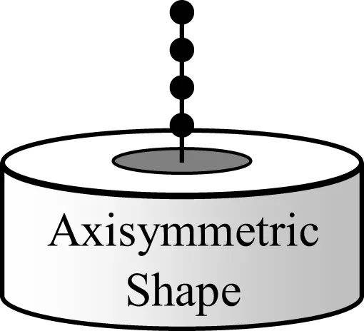 | 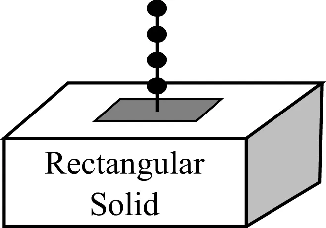 |
| Coordinate system | Axisymmetric | Orthogonal |
| Transmitting boundary | Theoretical method | Approximate method (proposed method) |
Shape of inner field and type of TB.
Accordingly, the TB should also be formulated using orthogonal coordinates rather than axisymmetric coordinates, but it is not possible to obtain such a theoretical solution. Therefore, an approximate 3D boundary model (hereinafter referred to as 3D-TB model) from a combination of a 2D in-plane problem TB (hereinafter referred to as SV-TB) and a 2D antiplane problem TB (Lysmer and Waas, 1972) (hereinafter referred to as SH-TB) is used.
At first, the outline of this model is explained. Next, a component of the model, the SH-TB, which has not been studied using time domain transform, is studied.
Then, the characteristics of soil impedance and input motion using 3D-TB are studied. Finally, time history response analysis of the 3D soil–structure interaction system using proposed 3D-TB model is conducted, and the effectiveness of the model is evaluated.
The VB, which is currently thought to be the most practical method for time domain analysis, is used for comparison in this study. Furthermore, it is known that accuracy is improved if the excavation force (EF) is applied to VB. EF is a correction force vector calculated as the product of free field soil displacements and frequency-independent stiffness matrix (refer to Supplementary Material). In order to further clarify the practical applicability of the proposed method, VB with EF is also compared in this study.
Outline of the Proposed Analysis Method
The TB is a highly accurate boundary model located at the outer side of the inner soil model, which is formed by parallel layers on the rigid bedrock. In a horizontal direction, the formulation is theoretical and rigorous. In a vertical direction, the formulation is approximate since it follows the element displacement assumption. The TB is able to almost completely absorb wave motion from an arbitrary direction. Even when the bottom of soil is semi-infinite condition, a favorable evaluation is possible by adding a sufficient amount of elements to the soil bottom, in the frequency domain.
In this paper, a time domain 3D-TB model, which corresponds to orthogonal coordinate system and uses SV-TB and SH-TB approximately, is proposed. An outline of this is described hereinafter.
Outline of the 3D-TB
The image of an inner field model is shown in Figure 2. In the figure, a vertical nodal group (hereinafter referred to as a “nodal line”) is considered on the boundary surface. This is placed as a basic unit to form the boundary model. The boundary surface is expressed as a collection of these nodal lines.
Figure 2
The control width of one nodal line extends to the center of the adjacent nodal lines. Both SV-TB and SH-TB are assigned in this nodal line (refer to Figure 3). Therefore, the degree of freedom within a nodal line is coupled, but the degree of freedom with the other nodal lines is not coupled. Theoretically, all nodal lines should be coupled with each other, but in the proposed model the efficiency of the calculation is improved by disregarding this.
Figure 3
Furthermore, if the soil properties are the same, each nodal line becomes a TB with identical properties, and only the control width is different. For this reason, a TB with a unit width nodal line that corresponds to the type of the soil properties is prepared. This is multiplied by the control width and assigned into the entire boundary surface.
The analysis flow is shown in Figure 4. The SH-TB and SV-TB are calculated in the frequency domain. These TB matrices are transformed to the time domains and assigned to the overall equation of motion.
Figure 4
Transform of TB Matrices to Time Domain
The reaction force from TB has to be calculated in the time domain. The calculation is not easy, because the components of the TB matrix are strongly frequency dependent. In this section, the concept of the transform of TB to the time domain and the obtained reaction force in the time domain are briefly explained, using a simple single DOF equation.
Although many methods to transform frequency dependent impedance function to the time domain have been proposed, most of them employed either the past displacement or the past velocity in the formulation of the impulse response. The author proposed transform methods using both the past displacement and velocity, then he confirmed that the accuracy of these methods is high (Nakamura, 2007, 2012a).
In this paper, the following methods were used for the transform. Here, Eq. 1 in the frequency domain is considered. Y(ω) is the reaction force, H(ω) is the frequency-dependent function (this corresponds to TB), and x(ω) is the displacement. The objective is to obtain the reaction force in the time domain y(t). In the proposed methods, Y(ω) and H(ω) are approximated by and as shown in Eq. 2. This equation is expressed as Eq. 3 in the time domain, where and x(t) are the reaction force and the displacement in the time domain, respectively.
tj = j Δt where Δt is the discrete time interval for the transform. 0hj, 1hj, and 2h0 are the coefficients of the impulse response. 0h0, 1h0, and 2h0 are called the simultaneous components, because they correspond to the current time t. 1h1 ~ 1hn’ and 0h1 ~ 0hn’ are called the time-delay components, since they correspond to the past time (t − tj). All of the unknown coefficients of the impulse response are obtained by simultaneous equations with given function data for H(ωi) (i = 0, 1, 2, …, N). This method is called as method B′.
In the case when the hysteretic damping is large, the accuracy of the transform tends to decrease. To improve this problem, the simultaneous components (2h0, 1h0, and 0h0) are corrected with (Δ2h0, Δ1h0, and Δ0h0), where Δ2h0, Δ1h0, and Δ0h0 indicate the modification terms determined by the least square method. The improved reaction force [ and ] can be expressed using Eqs 4 and 5. This method is called as method C′.
Using Eqs 4 and 5, all the components of [TB] can be transformed to the time domain. The details of the transform are shown in Nakamura (2007, 2012a).
Remarks for Application
With the method proposed in this paper, the nodal lines are mutually discontinuous as above. Therefore, it is thought that accuracy will decrease when the neighboring free field soil conditions differ greatly. Furthermore, it is necessary to calculate the SV-TB and SH-TB of the nodal line for each type of soil properties. Thus, when there are many types of soil properties, the calculation time increases, and the analysis becomes less efficient. For this reason, it is thought that the proposed method is effective when the types of soil properties are not so many.
Study of SH-TB
At first, the properties and applicability of the time domain SH-TB, which is a component of the 3D-TB model, are verified in preparation for analysis of this model. The applicability and accuracy of SV-TB was already confirmed in Nakamura (2009, 2012a).
Analysis Conditions
The analysis model is shown in Figure 5. The soil is multilayered with the shear velocity Vs in the range 200–400 m/s, on the bedrock with Vs = 500 m/s. A height difference of 10 m is set at one side of the soil (only left side). The characteristics of the bedrock are evaluated using the bottom VB in the inner field.
Figure 5
The building is represented by a lumped mass model with shear elements. Its width is 20 m, the height of above-ground part is 24 m, and the height of the underground part is 10 m. The causal hysteretic damping model (Nakamura, 2007) is used. The damping ratio is set to be 3% for the building and 2% for the soil. The material properties of the soil and the building are shown in Tables 2 and 3, respectively. In this paper, the soil properties and building materials of all analysis models are assumed to be stayed in the linear initial condition, because that can express the differences of the wave boundaries clearly.
Table 2
| Vs (m/s) | Poisson ratio ν | Density ρ (t/m3) | Damping ratio h | Thickness (m) | |
|---|---|---|---|---|---|
| Surface 1 | 200 | 0.4 | 2.0 | 0.02 | 20 |
| 2 | 300 | 10 | |||
| 3 | 400 | 10 | |||
| Bedrock | 500 | 0 | – |
Property of soil.
Table 3
| Story | Height (m) | Weight (t) | Rotational inertia (×105 t/m2) | Shear stiffness (×106 kN/m) |
|---|---|---|---|---|
| 6 | 4.0 | 480 | 0 | 0.4935 |
| 5 | 4.0 | 480 | 0 | 0.9047 |
| 4 | 4.0 | 480 | 0 | 1.234 |
| 3 | 4.0 | 480 | 0 | 1.480 |
| 2 | 4.0 | 480 | 0 | 1.645 |
| 1 | 4.0 | 480 | 0 | 1.727 |
| B1 | 5.0 | 720 | 0 | ∞ |
| B2 | 5.0 | 720 | 1.68 | ∞ |
Property of building.
Three analysis models, with the boundary at a distance of L = 5, 40, and 100 m from the building outer edge, were studied.
For estimating the semi-infinity of the bottom soil, the elements for 100 m height of the material properties of the bedrock were added to the lowest part of the soil model in the calculation of the TB matrix. The conditions for time domain transform for the TB matrix are shown in Table 4.
Table 4
| Impedance | Impulse response | |||
|---|---|---|---|---|
| No. of data | Frequencies of data (Hz) | Δt (s) | Simultaneous components | Time delay components |
| 21 | 0.1, 1.0, 2.0, 3.0, …, 19.0, 20.0 | 0.05 | k0, c0, m0 | k1 ~ k20, c1 ~ c19 |
Conditions for transform into the time domain.
The input ground motion was El Centro 1940NS wave (duration of 10 s, time step ΔT of 0.01 s), with the maximum acceleration set to 500 Gal and defined as 2E (double the ascending wave) at the bottom VB. As the time integral method, Newmark-β method (β = 1/4) was used.
Analysis Results
Figure 6 shows a comparison of the maximum response values (acceleration, displacement, and shear force) for the above-ground part of the building obtained by frequency domain and time domain analyses using the SH-TB. In each figure, the response results for each case are almost identical, and the results vary very slightly in accordance with L. Figure 7 shows the results of the time domain analysis using a VB. For comparison, the results of the TB for L = 100 m are also shown in the figure. The response results for each case are almost identical as are the results for the TB.
Figure 6
Figure 7
In the study of the SV problem (Nakamura, 2009, 2012b), the superiority of the TB is clearly displayed. However, it can be said that the difference between the TB and VB is slight in the case of the SH problem.
Incidentally, when input ground motion from a vertically downward direction is assumed for the SH problem, as it is in this analysis, EF is not required in the calculation.
Soil Impedance and Input Motion of the 3D-TB
The characteristics of soil impedance and input motion were evaluated in order to study the efficiency of the proposed 3D-TB. The same study was conducted with a VB as a target of comparison.
Analysis Conditions
The massless rigid foundation embedded in the multilayered soil is studied. The FEM analysis model is shown in Figure 8. This model is the soil model in the previous section transformed to 3D, and each dimension is the same. However, in this model, there is not a height difference at both sides of the soil, and the foundation is entirely embedded. Similarly to the previous section, two types of side boundary, 3D-TB and VB, were studied in the time domain at distances L of 5, 40, and 100 m between the outer edge of the foundation and the boundary.
Figure 8
Study of Soil Impedance
Impulse excitation was performed for the massless rigid foundation in order to calculate the time history wave for the displacement of the foundation. The impulse excitation consists of many different and constant frequency components (it is so-called as the white noise), so it is very convenient to study the frequency dependency of the given function in the time domain. The time integral method was the same as that described in the previous section. The impulse excitation time history wave and the foundation displacement time history wave were transformed using Fourier transformation, and the divisions for frequency domain were performed to calculate impedance. Two components of impedance – horizontal (Kx) and rotational (Kθy) – were studied. The thin-layer element method (TLEM) (Tajimi, 1980) is used as a target for comparison.
Figure 9 shows a comparison between TLEM results and the horizontal components of a soil impedance obtained using 3D-TB and VB. 3D-TB results in Figures 9A,B correspond favorably with TLEM totally, while slight fluttering can be seen when L = 5 and 40 m in the real part. In contrast, VB results in Figures 9C,D indicate that the difference with TLEM increases in the case of L = 5 m. The other cases generally correspond with TLEM, but the fluctuation in values for both the real part and imaginary part becomes greater in the vicinity of 0 Hz. This is thought to be because the bottom of the model is also VB, and therefore reaction force for excitation similar to static loading cannot be obtained.
Figure 9
For the rotational component in Figure 10, the tendency is almost the same. 3D-TB corresponds favorably with TLEM in all cases. The difference between VB and TLEM is large when L = 5 m, but in all other cases, VB generally corresponds favorably to TLEM.
Figure 10
Study of Input Motion
An impulse wave was applied as the input ground motion from the bottom of the model, and time history response analysis is conducted. The acceleration response wave is calculated at the center of the massless rigid foundation at soil surface level. The acceleration response and the time history wave of the impulse input motion are transformed to the frequency domain by Fourier transform, and divisions are performed to calculate the transfer function of the input motion. Two studies were conducted for VB, one when EF is applied and one when EF is not considered.
The analysis results are shown in Figure 11. For the 3D-TB in Figure 11A, the results for all cases of L are almost identical. In the case of VB without EF in Figure 11B, on the other hand, differences exist between each L case. In the results for L = 100 m, fluttering that was not apparent in Figure 11A can also be seen in the frequency range of 3–8 Hz. Figure 11C shows the results of the case of VB with FE. In all cases except for L = 5 m, the results of VB became almost identical with 3D-TB results. Thus, it is considered that the accuracy of VB is improved by EF.
Figure 11
Summary of Impedance and Input Motion
The accuracy of soil impedance and input motion was studied for the massless rigid foundation in the multilayered soil. The results when using 3D-TB were as follows.
- -
For soil impedance, the results corresponded favorably with the analytical solution (TLEM) generally. Although there was slight fluttering in the case of L = 5 and 40 m, the results were favorable totally.
- -
All cases are almost identical for input motion.
In contrast, the results when using VB were as follows.
- -
For soil impedance, there was a large difference in the case of L = 5 m. But for all other cases, the results generally corresponded favorably with the analytical solution.
- -
In the case of input motion, the disparity in each case was large when EF was not applied, and in all cases, the results differed from the results for the TB. Accuracy improved when EF was applied, and the results corresponded with the results for the TB in all cases except for L = 5 m.
Study of Time History Analysis Using 3D-TB
Time history seismic analysis of the soil and structure interaction system is conducted using the proposed 3D-TB, and the accuracy and the efficiency of the method are studied.
Analysis Conditions
The analysis model is shown in Figure 12. This model is the model from Figure 4 transformed to 3D. Therefore, the soil and building properties are the same as in Section “Study of SH-TB.” The input ground motion conditions and the time integration method are the same as in Section “Study of SH-TB,” but in this Section “Outline of the Proposed Analysis Method,” types of excitation are studied, excitation in the X and Y direction (hereafter referred as “X excitation” and “Y excitation”, respectively). The distance L from the outer edge of the building to the boundary is set as 5, 10, 20, 40, 60, 80, or 100 m, and the study conducted.
Figure 12
Comparison of Responses for the Soil Near the Building
The maximum response values (acceleration and displacement) for soil near the building when 3D-TB is used are shown in Figure 13A. Responses were compared for three cases, L = 5, 40, and 100 m. Although the maximum acceleration values of L = 5 m are slightly different to the other cases in Y excitation, the all values generally are almost identical in all cases for both X and Y excitations.
Figure 13
The maximum response values using VB without EF are shown in Figure 13B. The results for the 3D-TB at L = 100 m, which are thought to be the most accurate among all cases (hereafter referred as “the high-accuracy values”), are also shown in this figure.
The results for VB at L = 100 m almost correspond with the high-accuracy values. It can be ascertained from this that even with a VB, good accuracy can be achieved if a sufficiently large L is applied. On the other hand, the difference from the high-accuracy values becomes greater in the results for L = 5 and 40 m.
The results when VB with EF is used are shown in Figure 13C. Overall, the accuracy is improved compared to Figure 13B, and the values in the case of L = 40 m correspond favorably with the high-accuracy values. In a contrast, there is a large disparity in the case of L = 5 m. This is thought to be due to the effect of the difference in soil impedance in the previous section.
Comparison of Horizontal Response Values of the Building
Figure 14A shows the horizontal maximum response values (acceleration, displacement, and shear force) for the above-ground part of the building when 3D-TB is used. The same three cases as in the previous section, L = 5, 40, and 100 m, were compared. Although there are slight differences in some parts of acceleration values and shear force values between the case when L = 5 m, and the other cases for Y excitation, generally the results for all cases correspond favorably for both X and Y excitations.
Figure 14
Table 5a shows the ratios of these maximum values corresponding to the high-accuracy values. Black field in the table indicates that the maximum difference exceeds 20%, and gray field indicates that the maximum difference is from 10 to 20%. When the 3D-TB was used for analysis, the maximum difference for all response values was <10%, and favorable response results could be obtained even in the case of L = 5 m.
Table 5
| Case | Excitation | Acceleration | Displacement | Shear force |
|---|---|---|---|---|
| (a) TB | ||||
| L = 5 m | X | 0.93–1.01 | 0.95–1.01 | 0.97–1.01 |
| Y | 0.90–0.95 | 0.94–0.99 | 0.91–0.95 | |
| L = 40 m | X | 0.99–1.01 | 0.99–1.01 | 0.99–1.01 |
| Y | 0.96–0.99 | 0.97–1.00 | 0.97–0.97 | |
| (b) VB without EF | ||||
| L = 5 m | X | 0.73–0.91 | 0.91–1.06 | 0.75–0.84 |
| Y | 0.73–0.89 | 0.97–1.07 | 0.84–0.88 | |
| L = 40 m | X | 0.82–0.91 | 0.87–0.99 | 0.82–0.84 |
| Y | 0.79–0.92 | 0.87–0.98 | 0.79–0.84 | |
| L = 60 m | X | 0.89–0.92 | 0.91–0.99 | 0.90–0.92 |
| Y | 0.89–0.91 | 0.91–0.98 | 0.88–0.90 | |
| L = 80 m | X | 0.95–0.99 | 0.95–0.99 | 0.96–0.99 |
| Y | 0.96–0.98 | 0.96–0.98 | 0.96–0.97 | |
| (c) VB with EF | ||||
| L = 5 m | X | 0.71–0.90 | 0.82–0.94 | 0.73–0.82 |
| Y | 0.74–0.93 | 0.87–0.96 | 0.81–0.86 | |
| L = 10 m | X | 0.83–0.96 | 0.89–0.96 | 0.86–0.93 |
| Y | 0.83–0.96 | 0.93–0.98 | 0.92–0.95 | |
| L = 20 m | X | 0.94–0.98 | 0.94–0.99 | 0.95–0.98 |
| Y | 0.95–0.98 | 0.95–0.99 | 0.96–0.98 | |
| L = 40 m | X | 0.98–0.99 | 0.99–0.99 | 0.98–0.99 |
| Y | 0.96–1.00 | 0.98–0.99 | 0.96–0.98 | |
Comparison of maximum response of building.
Values in this table show the range of maximum responses (ratios to the response of TB, L = 100 m). The color of each field shows the maximum difference (black: >20%, gray: between 10 and 20%, and white: ≤10%).
The maximum response values for the above-ground part of the building when VB without EF is used are shown in Figure 14B. The results for VB at L = 100 m almost correspond with the high-accuracy values, but the results at L = 5 and 40 m are different significantly from the high-accuracy values. In Table 5b, the cases of L = 60 and 80 m are also included for comparison, in addition to the above cases. When using VB, the differences exceed 20% in some fields in the case of L = 5 and 40 m. Even at L = 60 m, the differences in half the fields exceeded 10%. The cases of L = ≥80 m, differences of all values are <10%. The results when using VB with EF are shown in Figure 14C. Although the differences are large at L = 5 m, the accuracy is favorable at L = 40 m. In Table 5c, the cases of L = 10 and 20 m are also included for comparison. In the cases of L = ≥20 m, all differences are <10%.
Figure 15 shows the transfer function of the response acceleration at the top node of the building for the input ground motion. When 3D-TB is used, shown in Figure 15A, the results for the values of both L = 5 and 40 m corresponded favorably with those of L = 100 m. When VB without EF was used, there is a significant difference in terms of the peak height between the cases of L = 5 and 100 m, as shown in Figure 15B. Between the cases of L = 40 and 100 m, the peak height and positions corresponded to each other, but a difference can be seen at 1.9–2.5 Hz. When the EF was applied to VB, as shown in Figure 15C, the accuracy for L = 40 m improved.
Figure 15
However, the accuracy for L = 5 m remained poor, as shown in Figure 15B. These results correspond to the tendency shown in Figures 14A–C.
Summary of Response Behavior
The above tendency is consistent with the results in Section “Soil Impedance and Input Motion of the 3D-TB.” Thus, the following can be concluded.
- -
When the 3D-TB is used, response accuracy is favorable even when L is small. This is thought to be because the accuracy for both soil impedance and input motion is high. The horizontal response accuracy was favorable (the difference is <10%) at L = 5 m (1/4 of the building width).
- -
When VB without EF is used, the accuracy of the response results is low at L = 5 and 40 m. This is thought to be because the accuracy of both soil impedance and input motion are low at L = 5 m, and the accuracy of input motion is low at L = 40 m. The horizontal response accuracy was favorable at L = 80 m (four times the building width).
- -
When VB with EF is used, the response values at L = 40 m become favorable. This is thought to be because the accuracy of the input motion is improved due to the application of EF. On the other hand, the accuracy at L = 5 m remained low. This is thought to be because of the low accuracy of the soil impedance. The horizontal response accuracy was favorable at L = 20 m (one time the building width).
Study of Analysis Load
Table 6 provides a comparison of the analysis loads for the cases that provided favorable horizontal response results for the building in Table 5, the case of L = 5 m of 3D-TB, the case of L = 80 m of VB without FE, and the case of L = 20 m of VB with EF. Model shapes of L = 5, 20, and 80 m are shown in Figure 16.
Table 6
| L (m) | No. of node | No. of elem. | Required memory (GB) | Analysis time (min) | |
|---|---|---|---|---|---|
| TB | 5 | 6,675 | 5,520 | 1.3 | 39 |
| VB without EF | 80 (16.0) | 195,135 (29.2) | 184,336 (33.4) | 18.0 (13.8) | 516 (13.2) |
| VB with EF | 20 (4.0) | 23,631 (3.5) | 21,136 (3.8) | 2.4 (1.8) | 71 (1.8) |
Comparison of analysis load (cases whose differences of building response are <10%).
The values in the parenthesis mean the magnification to TB.
Figure 16
As for the analysis load, the required memory size and the analysis time during the calculation were counted using a single core Xeon7560 (2.26 GHz) processor. This processing unit has 256 GB of main memory space, and the calculations for all cases were conducted within the main memory. Furthermore, the 3D-TB calculation time in the frequency domain and the time domain transform time (total for both for the SV problem and the SH problem is 1.2 min) are included in the 3D-TB analysis time.
Compared to VB (without EF) case, the 3D-TB case has around 1/30 of the number of inner field nodal points and elements. It is also ~1/13 of the memory and analysis time. Furthermore, this required memory and analysis time is reduced to approximately half that required in the case of VB with EF applied.
Conclusion
In this paper, an approximate time domain TB that can be used with a 3D orthogonal coordinate system was studied. First, 3D-TB with high calculation efficiency that can be applied in a rectangular analysis domain was explained. A nodal line on the boundary surface is considered to be a single unit, and the SV-TB and the SH-TB are assigned to it.
Next, the properties of the component, the SH-TB, were studied and verified for favorable accuracy. Then the impedance and input motion of the rigid foundation embedded in the multilayered soil were calculated using the 3D-TB, and favorable correspondence with the analysis solution was obtained.
Furthermore, seismic response analysis of the 3D problem was conducted using the proposed 3D-TB. From the aspect of the accuracy of horizontal response values, improvement effects were obtained at ~1/13 of the required memory and analysis time compared to VB without EF and approximately half of the required memory and analysis time compared to VB with EF. It can be concluded from this that the effectiveness of the proposed 3D-TB has been confirmed.
Statements
Conflict of interest
The author declares that the research was conducted in the absence of any commercial or financial relationships that could be construed as a potential conflict of interest.
Supplementary material
The Supplementary Material for this article can be found online at http://journal.frontiersin.org/article/10.3389/fbuil.2015.00021
References
1
BasuU.ChopraA. K. (2004). Perfectly matched layers for transient elastodynamics of unbounded domains. Int. J. Numer. Methods Eng.59, 1039–1074.10.1002/nme.896
2
BerengerJ. P. (1994). A perfectly matched layer for the absorption of electromagnetic wave. J. Comput. Phys.114, 185–200.10.1006/jcph.1994.1159
3
FattahM. Y.SchanzT.DawoodS. H. (2012). The role of transmitting boundaries in modeling dynamic soil-structure interaction problems. Int. J. Eng. Technol.2, 236–258.
4
GherguM.IonescuI. R. (2009). Structure-soil-structure coupling in seismic excitation and city effect. Int. J. Eng. Sci.47, 342–354.10.1016/j.ijengsci.2008.11.005
5
GuidottiR.MazzieriI.StupazziniM.DagnaP. (2012). “3D numerical simulation of the site-city interaction during the 22 February 2011 MW 6.2 Christchurch earthquake,” in 15th World Conference of Earthquake Engineering. Lisbon.
6
HastingsF. D.SchneiderJ. B.BroschatS. L. (1996). Application of the perfectly matched layer (PML) absorbing boundary condition to elastic wave propagation. J. Acoust. Soc. Am.100, 3061–3069.10.1121/1.417118
7
KimD. K.YunC. B. (2000). Time domain soil-structure interaction analysis in two – dimensional medium based on analytical frequency – dependent infinite elements. Eng. Struct.22, 258–271.10.1016/S0141-0296(98)00070-4
8
LouM.WangH.ChenX.ZhaiY. (2011). Structure-soil-structure interaction: literature review. Soil Dyn. Earthquake Eng.31, 1724–1731.10.1016/j.soildyn.2011.07.008
9
LysmerJ.KuhlelameyerR. L. (1969). Finite dynamic model for infinite area. J. Eng. Mech. Div.95, 859–877.
10
LysmerJ.UdakaT.SeedH. B.HwangR.N. (1975a). FLUSH A Computer Program for Approximate 3-D Analysis of Soil-Structure Interaction Problems. Report No.EERC75-30. Berkeley, CA: University of California.
11
LysmerJ.UdakaT.TsaiC.-F.SeedH. B. (1975b). ALUSH A Computer Program for Seismic Response Analysis of Axisymmetric Soil-Structure Systems. Report No.EERC75-31. Berkeley, CA: University of California.
12
LysmerJ.WaasG. (1972). Shear wave in plane infinite structures. J. Eng. Mech. Div.98, 85–105.
13
MillanM. A.DominguezJ. (2009). Simplified BEM/FEM model for dynamic analysis of structures on piles and pile group in viscoelastic and poroelastic soils. Eng. Anal. Bound. Elem.33, 25–34.10.1016/j.enganabound.2008.04.003
14
NakamuraN. (2006). Improved methods to transform frequency dependent complex stiffness to time domain. Earthquake Eng. Struct. Dyn.35, 1037–1050.10.1002/eqe.520
15
NakamuraN. (2007). Practical causal hysteretic damping. Earthquake Eng. Struct. Dyn.36, 597–617.10.1002/eqe.644
16
NakamuraN. (2009). Nonlinear response analysis of soil-structure interaction system using transformed energy transmitting boundary in the time domain. Soil Dyn. Earthquake Eng.29, 799–808.10.1016/j.soildyn.2008.08.004
17
NakamuraN. (2012a). A basic study on the transform method of frequency dependent functions into time domain – relation to Duhamel’s integral and time domain transfer function. J. Eng. Mech.138, 276–285.10.1061/(ASCE)EM.1943-7889.0000330
18
NakamuraN. (2012b). Two-dimensional energy transmitting boundary in the time domain. Int. J. Earhquakes Struct.3, 97–115.10.12989/eas.2012.3.2.097
19
PadronL. A.AznarezJ. J.MaesoO. (2011). 3-D boundary element – finite element method for the dynamic analysis of piled buildings. Eng. Anal. Bound. Elem.35, 465–477.10.1016/j.enganabound.2010.09.006
20
SmithW. (1973). A non-reflecting plane boundary for wave propagation problems. J. Comput. Phys.15, 492–503.10.1016/0021-9991(74)90075-8
21
TajimiH. (1980). “A contribution to theoretical prediction of dynamic stiffness of surface foundations,” in Proceeding of 7th World Conference on Earthquake Engineering (Istanbul), 105–112.
22
WolfJ. P. (2003). The Scaled Boundary Finite Element Method. West Sussex: John Wiley & Sons Ltd.
23
WolfJ. P.SongC. (1996). Finite-Element Modelling of Unbounded Media. West Sussex: John Wiley & Sons Ltd.
Summary
Keywords
energy transmitting boundary, FEM, time domain, three-dimensional analysis, soil–structure interaction, viscous boundary
Citation
Nakamura N (2015) Three-Dimensional Energy Transmitting Boundary in the Time Domain. Front. Built Environ. 1:21. doi: 10.3389/fbuil.2015.00021
Received
23 June 2015
Accepted
19 October 2015
Published
03 November 2015
Volume
1 - 2015
Edited by
Nikos D. Lagaros, National Technical University of Athens, Greece
Reviewed by
Vagelis Plevris, School of Pedagogical and Technological Education, Greece; Sameh Samir F. Mehanny, Cairo University, Egypt; Anaxagoras Elenas, Democritus University of Thrace, Greece
Updates
Copyright
© 2015 Nakamura.
This is an open-access article distributed under the terms of the Creative Commons Attribution License (CC BY). The use, distribution or reproduction in other forums is permitted, provided the original author(s) or licensor are credited and that the original publication in this journal is cited, in accordance with accepted academic practice. No use, distribution or reproduction is permitted which does not comply with these terms.
*Correspondence: Naohiro Nakamura, nakamura.naohiro@takenaka.co.jp
Specialty section: This article was submitted to Earthquake Engineering, a section of the journal Frontiers in Built Environment
Disclaimer
All claims expressed in this article are solely those of the authors and do not necessarily represent those of their affiliated organizations, or those of the publisher, the editors and the reviewers. Any product that may be evaluated in this article or claim that may be made by its manufacturer is not guaranteed or endorsed by the publisher.