Critical Response of 2DOF Elastic–Plastic Building Structures under Double Impulse as Substitute of Near-Fault Ground Motion

Introduction

The effects of near-fault ground motions on structural response have been investigated extensively (Bertero et al., 1978; Singh, 1984; Hall et al., 1995; Iwan, 1997; Sasani and Bertero, 2000; Alavi and Krawinkler, 2004; Makris and Black, 2004; Mavroeidis et al., 2004; Kalkan and Kunnath, 2006, 2007; Xu et al., 2007; Rupakhety and Sigbjörnsson, 2011; Yamamoto et al., 2011; Minami and Hayashi, 2013; Vassiliou et al., 2013; Khaloo et al., 2015; Vafaei and Eskandari, 2015). The fling-step and forward-directivity are widely recognized as special keywords to characterize such near-fault ground motions (Mavroeidis and Papageorgiou, 2003; Bray and Rodriguez-Marek, 2004; Makris and Black, 2004; Kalkan and Kunnath, 2006; Mukhopadhyay and Gupta, 2013a,b; Zhai et al., 2013; Hayden et al., 2014; Yang and Zhou, 2014). Especially, after Northridge earthquake in 1994, Hyogoken-Nanbu (Kobe) earthquake in 1995 and Chi-Chi (Taiwan) earthquake in1999, a strong interest has been taken by many earthquake structural engineers. The fling-step and forward-directivity are widely recognized special keywords to characterize such near-fault ground motions. The fling-step and forward-directivity inputs have been characterized by two or three wavelets. For this class of ground motions, many useful research works have been conducted. Mavroeidis and Papageorgiou (2003) investigated the characteristics of this class of ground motions in detail and proposed some simple models (for example, Gabor wavelet and Berlage wavelet). Makris and Black (2004) investigated the effects of two or three wavelets on structural inelastic responses. Kalkan and Kunnath (2006) introduced two or three simple sinusoidal wavelets based on the research of Sasani and Bertero (2000) and investigated the influence of near-fault ground motions on tall buildings. Xu et al. (2007) employed a kind of Berlage wavelet and applied it to the performance evaluation of passive energy dissipation systems. Takewaki and Tsujimoto (2011) used the Xu’s approach and proposed a method for scaling ground motions from the viewpoints of drift and input energy demand. Afterwards, Takewaki et al. (2012) employed a sinusoidal wave for pulse-type waves.

Most of the previous works on the near-fault ground motions deal with the elastic response except Mavroeidis et al. (2004), Makris and Black (2004), Kalkan and Kunnath (2006, 2007), Vassiliou et al. (2013), and Khaloo et al. (2015), because the number of parameters (e.g., duration and amplitude of pulse, ratio of pulse frequency to structure natural frequency, change of equivalent natural frequency for the increased input level) to be considered on this topic is many and the computation itself of elastic–plastic responses is quite complicated.

Kojima and Takewaki (2015a,b) recently derived some closed-form solutions of the critical response of single-degree-of-freedom (SDOF) elastic–plastic structures under such two or three wavelets (double or triple impulses). The amplitude of the double impulse was modulated so that its maximum Fourier amplitude coincides with that of the corresponding one-cycle sinusoidal input (Kojima and Takewaki, 2015a). It was shown that, since only the free-vibration appears under such double impulse input, the energy approach plays an important role in the derivation of the closed-form solution of a complicated elastic–plastic response. The extension of the theory for the fling-step near-fault ground motion to the forward-directivity near-fault ground motion was made by Kojima and Takewaki (2015b). Furthermore, Kojima and Takewaki (2015c) extended their approach to long-duration ground motions. This approach is based on an innovative concept of transformation of input and unchanged treatment of an elastic–plastic structure itself compared to the conventional equivalent linearization method for elastic–plastic structures and has overcome a difficulty encountered for elastic-perfectly plastic structures since 1960 (Caughey, 1960a,b; Iwan, 1961, 1965a,b; Liu, 2000).

In the earthquake-resistant design of structures, the resonance is a key concept and it has been investigated extensively. While the resonant equivalent frequency must be computed for a specified input level by changing the excitation frequency in a parametric manner for the sinusoidal input (Caughey, 1960a,b; Iwan, 1961, 1965a,b; Roberts and Spanos, 1990; Liu, 2000), no iteration is needed in the method for the double impulse (Kojima and Takewaki, 2015a,c). This is because the resonant equivalent frequency can be derived directly without the repetitive procedure. In the double impulse, the analysis can be done without the concept of the input frequency (timing of impulses) before the second impulse. The resonance can be proved by using energy balance and the timing of the second impulse can be characterized as the time with zero restoring force. The maximum elastic–plastic response after impulse can be obtained by equating the initial kinetic energy computed by the initial velocity to the sum of hysteretic and elastic strain energies. It should be pointed out that only critical response (upper bound) is captured by the method and the critical resonant frequency can be obtained automatically for the increasing input level of the double impulse.

The double impulse is introduced here as a substitute of the fling-step near-fault ground motion and a critical elastic–plastic response of a 2DOF building structure under the “critical double impulse” is evaluated. The input of impulse is expressed by the instantaneous change of velocities of the structural masses. Since only the free-vibration appears under such double impulse, the energy balance approach plays an important role in the derivation of the solution of a complicated elastic–plastic critical response as in Kojima and Takewaki (2015a–c). It is shown that the critical timing of the double impulse is characterized by the timing of the second impulse at the zero story shear force in the first story. This criticality is also characterized by the maximization of the sum of the momenta of all masses. This timing certainly guarantees the maximum energy input by the second impulse that causes the maximum plastic deformation after the second impulse. Because the response of 2DOF elastic–plastic building structures is quite complicated due to the phase difference between two masses compared to SDOF models for which a closed-form critical response can be derived, the upper bound of the critical response is introduced by using the convex model (Ben-Haim and Elishakoff, 1990; Ben-Haim et al., 1996). The accuracy of the derived upper bound is discussed in comparison with the actual response analysis result to the double impulse. The validity and accuracy of the proposed theory for the double impulse are also investigated through the comparison with the response analysis result to the corresponding one-cycle sinusoidal input as a representative of the fling-step near-fault ground motion.

Double Impulse Input

The fling-step input (fault-parallel) of the near-fault ground motion can be represented by a one-cycle sinusoidal wave and the forward-directivity input (fault-normal) of the near-fault ground motion can be expressed by a series of three sinusoidal wavelets as pointed out in the reference (Kojima et al., 2015 and Kojima and Takewaki, 2015a) (see Figure 1). It has further been pointed out (Makris and Black, 2004) that a one-cycle sinusoidal wave can also express the forward-directivity input in some cases. In this paper, it is aimed at simplifying the typical near-fault ground motions by a double impulse (Kojima et al., 2015; Kojima and Takewaki, 2015a).

FIGURE 1

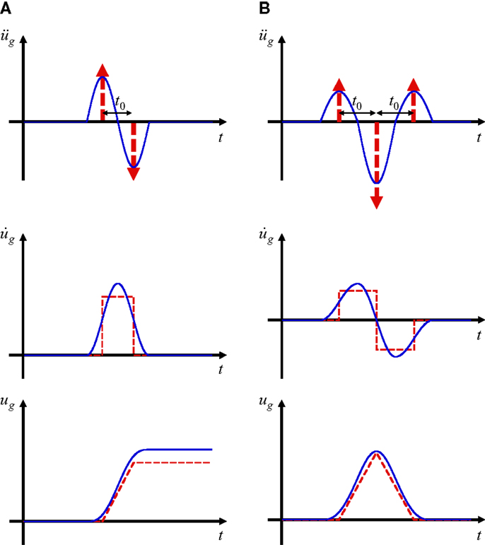
Figure 1. (A) Fling-step input and double impulse, (B) Forward-directivity input and triple impulse (Kojima and Takewaki, 2015a).

Consider a double impulse ground acceleration ${\ddot{u}}_g(t)$, as shown in Figure 1A, expressed by

${\ddot{u}}_g(t)=V\delta (t)-V\delta (t-t_0),$ (1)

where V is the given velocity and t₀ is the time interval between two impulses. The time derivative is denoted by an over-dot. The comparison with the corresponding one-cycle sinusoidal wave as a representative main part of the near-fault ground motion is plotted in Figure 1A (Mavroeidis and Papageorgiou, 2003; Makris and Black, 2004; Kalkan and Kunnath, 2006; Kojima and Takewaki, 2015a). The corresponding velocity and displacement of such double impulse and sinusoidal wave are also plotted in Figure 1A. As pointed out earlier, the double impulse is a good approximation of the corresponding sinusoidal wave even in the form of velocity and displacement on the condition that the correspondence of the maximum Fourier amplitude is guaranteed (see Appendix 1). It may be interesting to note that, since the Fourier amplitude is related to the velocity of ground motions (or velocity response spectrum), this correspondence is meaningful.

The Fourier transform of ${\ddot{u}}_g(t)$ of the double impulse input can be expressed as

$\begin{array}{ll}{\ddot{U}}_g(\omega )& ={\displaystyle {\int }_{-\infty }^{\infty }\left\{V\delta (t)-V\delta (t-t_0)\right\}{e}^{-\text{i}\omega t}}dt\\ & ={\displaystyle {\int }_{-\infty }^{\infty }\left\{V\delta (t)e^{-\text{i}\omega t}-V\delta (t-t_0)e^{-\text{i}\omega t_0}{e}^{-\text{i}\omega (t-t_0)}\right\}}dt\\ & =V\text{(}1-e^{-\text{i}\omega t_0}).\end{array}$ (2)

2DOF System and Normalization of Double Impulse

Consider an undamped elastic-perfectly plastic two-degree-of-freedom (2DOF) system, as shown in Figure 2, subjected to the above-mentioned double impulse. Let m_i and k_i denote the i-th story mass and stiffness, respectively. The yield deformation and yield force of the i-th story are denoted by d_yi and f_yi. Let, ω₁, u_i, d_i, and f_i denote the undamped fundamental natural circular frequency of the 2DOF system, the displacement of the i-th story mass relative to the ground, the interstory drift of the i-th story, and the restoring force of the i-th story, respectively. The velocity of mass is also denoted by $v_i={\dot{u}}_i$.

FIGURE 2

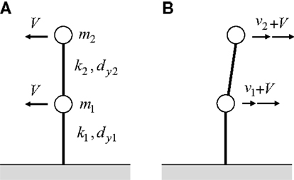
Figure 2. Undamped elastic-perfectly plastic 2DOF system subjected to double impulse. (A) First impulse. (B) Second impulse.

The reference value V_y of the velocity of the input double impulse is selected so that the input initial kinetic energy is transformed into the sum of the elastic limit strain energies.

$\frac{1}{2}\left(m_1+m_2\right)V_y{}^2=\frac{1}{2}{k}_1{d}_{y1}^2+\frac{1}{2}{k}_2{d}_{y2}^2.$ (3)

Although the interstory drifts of the first and second stories do not usually attain the elastic limit simultaneously, this state is used merely for normalizing the input level. Figure 3 shows an example of the time histories of the restoring forces in the first and second stories for a model of equal mass, equal story stiffness, and equal yield interstory drift subjected to the single impulse at t = 0 with V/V_y = 1. The response has been computed by using the Newmark-beta method.

FIGURE 3

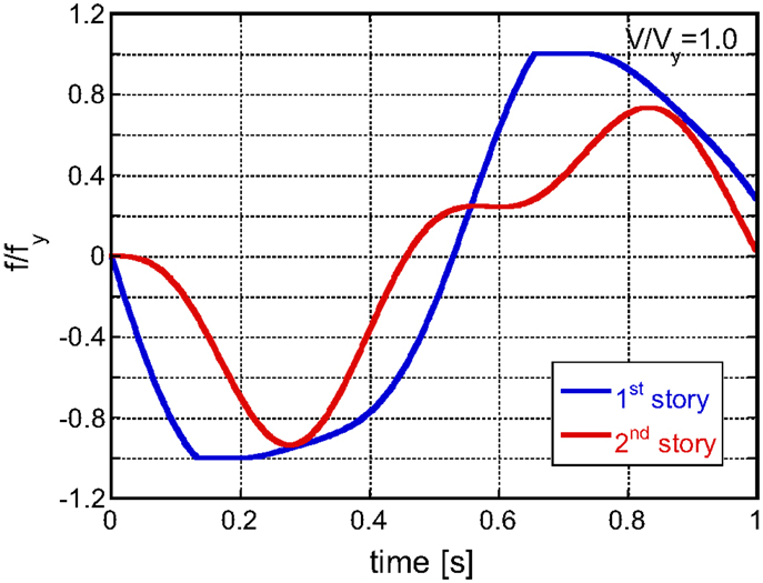
Figure 3. Example of the time histories of the restoring forces in the first and second stories for a model of equal mass, equal story stiffness, and equal yield interstory drift subjected to the single impulse at t = 0 with V/V_y = 1.0.

Description of Elastic–Plastic Response Process in Terms of Energy Quantities

It may be convenient to describe the key phases in terms of symbols as shown in Figure 4. Let $d_{i\max }^{(1)}$ and $d_{i\max }^{(2)}$ denote the maximum interstory drift after the first impulse and that after the second impulse, respectively, in the i-th story and let $d_{pi}^{(1)}$ and $d_{pi}^{(2)}$ denote the plastic deformation after the first impulse and that after the second impulse, respectively, in the i-th story. The phase (A) indicates the state in which the first interstory drift attains the maximum value in the plastic region after the first impulse. The phase (B) presents the state just before the input of the second impulse and the phase (C) expresses the state just after the input of the second impulse. Furthermore, the phase (D) indicates the state in which the first interstory drift attains the maximum value in the other-side plastic region after the second impulse. The phase (B) with zero first-story restoring force in Figure 4 has been introduced because this timing plays an important role in Section “Maximization of ΔE (Minimization of ΔE in Addition).”

FIGURE 4

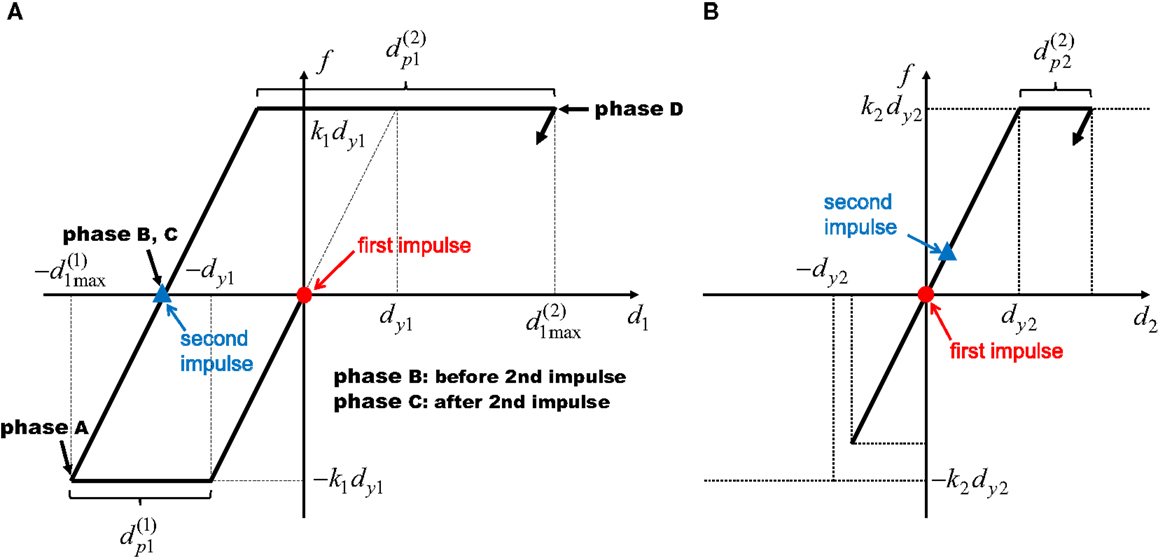
Figure 4. Key phases (A), (B), (C), and (D) in the restoring-force characteristics. (A) First story. (B) Second story.

In the phase (A), the velocity of the first-story mass is 0. Let $E_2^{(A)}$ denote the sum of the elastic strain energy of the second story and the kinetic energy of the second-story mass. Although $E_2^{(A)}$ does not necessarily represent the total mechanical energy of the second story, it is called the “total mechanical energy of the second story” for simplicity. In this case, the total mechanical energy $E_{sum}^{(A)}$ of the whole system at the phase (A) (the dissipated energy in the first story is not included because this is not the mechanical energy) can be expressed as

$E_{sum}^{(A)}=\frac{1}{2}{k}_1{d}_{y1}^2+E_2^{(A)}.$ (4)

Since the mechanical energy is conserved from the phase (A) to the phase (B) [$E_{sum}^{(B)}$: total mechanical energy at the phase (B)], the following relation holds.

$E_{sum}^{(B)}=E_{sum}^{(A)}.$ (5)

Let ΔE denote the energy input by the second impulse. In this case, the total mechanical energy $E_{sum}^{(C)}$ at the phase (C) can be related to $E_{sum}^{(B)}$ as follows.

$E_{sum}^{(C)}=E_{sum}^{(B)}+\Delta E.$ (6)

Let $E_2^{(D)}$ denote the sum of the elastic strain energy of the second story and the kinetic energy of the second-story mass at the phase (D). In this case, the total mechanical energy $E_{sum}^{(D)}$ at the phase (D) can be related to $E_2^{(D)}$ as follows:

$E_{sum}^{(D)}=\frac{1}{2}{k}_1{d}_{y1}^2+E_2^{(D)}.$ (7)

The energy balance provides

$E_{sum}^{(C)}=E_{sum}^{(D)}+k_1{d}_{y1}{d}_{p1}^{(2)}+k_2{d}_{y2}{d}_{p2}^{(2)}.$ (8)

It may be rare that the second story goes into the plastic region after the second impulse (this issue will be discussed later in Section “Input Level for Loose Upper Bound”). Therefore $d_{p2}^{(2)}$ = 0 in most cases. Substitution of Eqs. 4, 5, 7, 8 into Eq. 6 yields

$\frac{1}{2}{k}_1{d}_{y1}^2+E_2^{(A)}+\Delta E=\frac{1}{2}{k}_1{d}_{y1}^2+E_2^{(D)}+k_1{d}_{y1}{d}_{p1}^{(2)}+k_2{d}_{y2}{d}_{p2}^{(2)}.$ (9)

From Eq. 9, the normalized plastic deformation of the first story after the second impulse can be expressed by

$\frac{d_{p1}^{(2)}}{d_{y1}}=\frac{1}{k_1{d}_{y1}^2}\left\{E_2^{(A)}+\Delta E-\left(E_2^{(D)}+k_2{d}_{y2}{d}_{p2}^{(2)}\right)\right\}.$ (10)

It can be understood from Eq. 10 that the upper bound of the plastic deformation $d_{p1}^{(2)}$ of the first story after the second impulse is derived by maximizing $E_2^{(A)}$ and ΔE and minimizing $E_2^{(D)}$ and $d_{p2}^{(2)}$. These manipulations will be discussed in the following. Since the 2DOF system includes some uncertain factors for state determination different from SDOF systems, the investigation on upper bound of responses may be meaningful (Takewaki, 1996, 1997, 2002).

Only critical response is taken into account by the proposed method and the critical resonant frequency can be obtained without iteration for the increasing input level as shown in Section “Upper Bound of Plastic Deformation in the First Story after the Second Impulse.” One of the original points in this paper is the introduction of the concept of “critical excitation” in the elastic–plastic response for multi-degree-of-freedom (MDOF) systems (Drenick, 1970; Abbas and Manohar, 2002; Takewaki, 2007; Moustafa et al., 2010). Once the frequency and amplitude of the critical double impulse are computed, the corresponding one-cycle sinusoidal motion can be identified.

Upper Bound of Plastic Deformation in the First Story after the Second Impulse

Maximization of $E_2^{(A)}$

Consider the situation where the first story is in the plastic loading range and the second story is in the elastic range after the first impulse. This case is often encountered in usual situations (for example, Bertero et al., 1978) and some examples will be shown for the model of equal mass, equal story stiffness, and equal yield interstory drift. In this case, the equations of motion after the yielding of the first story, i.e., until phase (A), can be described by

$\begin{array}{l}{m}_1{\ddot{u}}_1-k_2\left(u_2-u_1\right)=k_{1}d{y}_1\\ m_2{\ddot{u}}_2+k_2\left(u_2-u_1\right)=0.\end{array}$ (11a,b)

Arrangement of Eqs. 11a,b leads to

$m_1{m}_2\left({\ddot{u}}_2-{\ddot{u}}_1\right)+k_2\left(m_1+m_2\right)\left(u_2-u_1\right)=-m_2{k}_{1}d{y}_1.$ (12)

The general solution of the differential equation, Eq. 12, can be expressed by

$u_2-u_1=-B\cos \left(\omega t+\delta \right)-A,$ (13)

where B is an undetermined coefficient and

$\omega =\sqrt{\frac{\left(m_1+m_2\right)k_2}{m_1{m}_2}},A=\frac{m_2{k}_1}{(m_1+m_2)k_2}d{y}_1.$ (14a,b)

Equation 13 indicates that the second-story interstory drift exhibits a simple harmonic vibration around the center of magnitude A as shown in Figure 5. Since the first story goes into the plastic range quickly and the second-story interstory drift has a zero initial value, the absolute minimum value of the second-story interstory drift is nearly 0. It can be shown that this assumption is a good approximation.

FIGURE 5

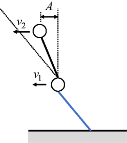
Figure 5. Simple harmonic vibration of the second-story mass around the center of magnitude A.

In this case, the following relation holds.

$B\doteq A$ (15)

$u_2-u_1\doteq -A\left\{\cos \left(\omega t+\delta \right)+1\right\}(\delta :\text{\hspace{0.17em}phase\hspace{0.17em}angle}).$ (16)

Then the condition that the second story does not go into the plastic range after the first impulse can be expressed by

$2A=\frac{2m_2{k}_1}{(m_1+m_2)k_2}d{y}_1\le d{y}_2.$ (17)

The model of equal mass, equal story stiffness, and equal yield deformation satisfies this condition.

Some examples of the time histories of the restoring forces in the first and second stories for a model of equal mass, equal story stiffness, equal yield interstory drift subjected to the single impulse at t = 0 with V/V_y = 1.15, 1.5, 2, 4 are shown in Figure 6. As in the previous numerical example, the response has been computed by using the Newmark-beta method. From these numerical investigations (Figure 6), the following relation can be derived approximately.

$\frac{m_2{k}_1}{(m_1+m_2)k_2}d{y}_1=\frac{1}{2}d{y}_1.$ (18)

FIGURE 6

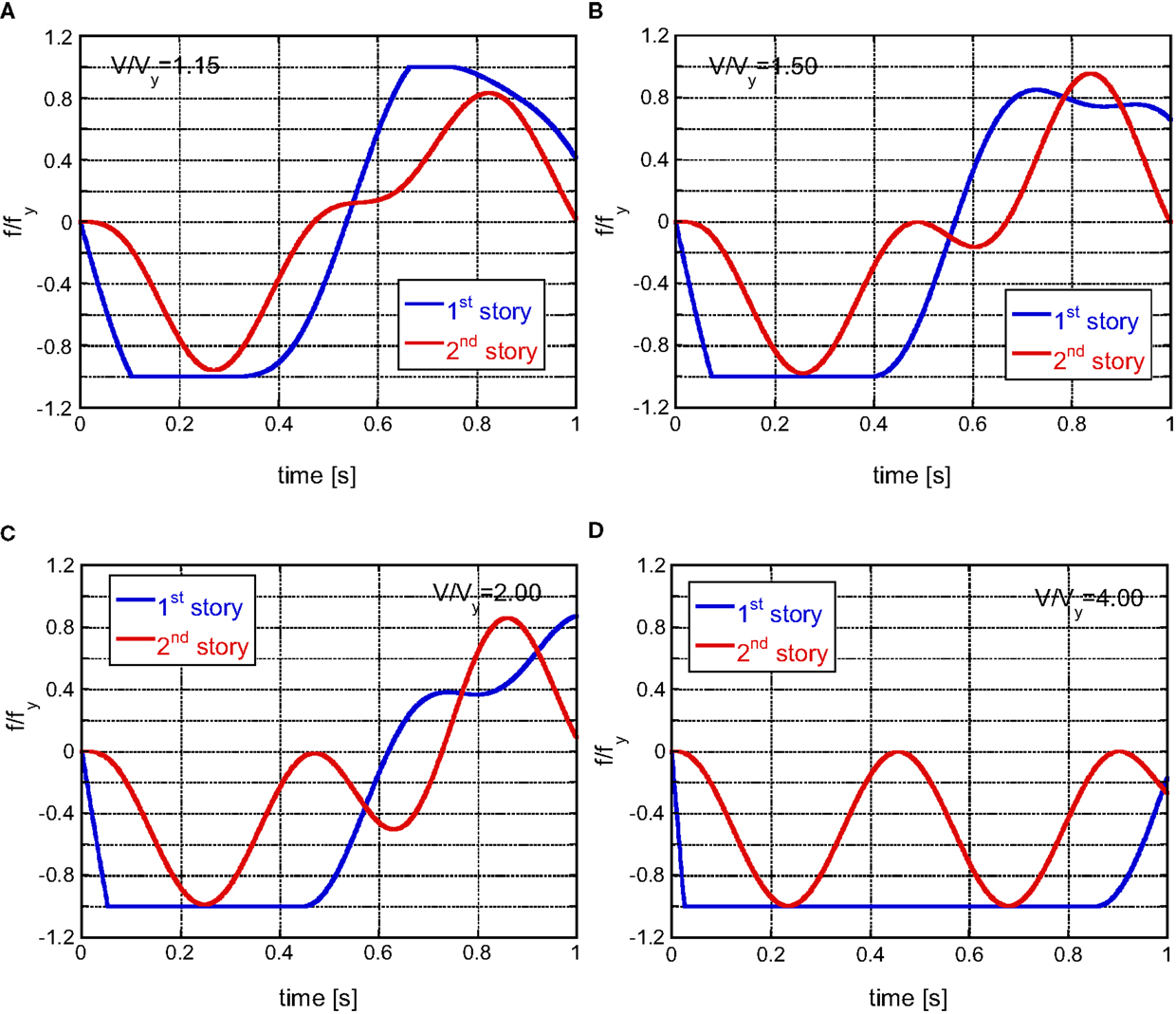
Figure 6. Examples of the time histories of the restoring forces in the first and second stories for a model of equal mass, equal story stiffness, and equal yield interstory drift subjected to the single impulse at t = 0 with V/V_y = 1.15, 1.5, 2, 4. (A) V/V_y = 1.15 (B) V/V_y = 1.5. (C) V/V_y = 2.0. (D) V/V_y = 4.0.

Equation 16 can also be expressed by

${\dot{u}}_2-{\dot{u}}_1\doteq A\omega \sin \left(\omega t+\delta \right).$ (19)

Since the first-story mass is at rest in the phase (A), the velocity of the second-story mass can be described by

${\dot{u}}_2=A\omega \sin \left(\omega t+\delta \right).$ (20)

Let us introduce the notation μ = m₂/m₁, κ = k₂/k₁. The total mechanical energy in the second story at the phase (A) can then be derived by

$E_2^{(A)}=\frac{1}{2}{k}_2{\left(u_2-u_1\right)}^2+\frac{1}{2}{m}_2{\dot{u}}_2^2.$ (21)

Substitution of Eqs. 16 and 20 into Eq. 21 leads to

$\begin{array}{ll}{E}_2^{(A)}& =\frac{1}{2}{A}^2\left[k_2{\left\{\cos \left(\omega t+\delta \right)+1\right\}}^2+m_2{\omega }^2{\sin }^2\left(\omega t+\delta \right)\right]\\ & =\frac{1}{2}{k}_2{A}^2\left[{\left\{\cos \left(\omega t+\delta \right)+1\right\}}^2+\left(\mu +1\right){\sin }^2\left(\omega t+\delta \right)\right]\\ & =\frac{1}{2}{k}_2{\left\{\frac{\mu }{\mu +1}\frac{1}{\kappa }{d}_{y1}\right\}}^2\left[-\mu {\left\{\cos \left(\omega t+\delta \right)-\frac{1}{\mu }\right\}}^2+\frac{1}{\mu }{\left(\mu +1\right)}^2\right].\end{array}$ (22)

In Eq. 22, the minimization of {cos (ωt + δ) − (1/μ)}² leads to the maximization of $E_2^{(A)}$. Since $0\le \left|\cos \left(\omega t+\delta \right)\right|\le 1$, it is necessary to consider two cases μ > 1 and μ ≤ 1. In case of μ > 1, cos (ωt + δ) − (1/μ) = 0 minimizes {cos (ωt + δ) − (1/μ)}². On the other hand, in case of μ ≤ 1, cos (ωt + δ) = 1 minimizes {cos (ωt + δ) − (1/μ)}².

Finally the following relations can be drawn.

$0\le E_2^{(A)}\le E_{2\max }^{(A)},$ (23)

where $E_{2\max }^{(A)}$ is the upper bound of $E_2^{(A)}$ and is given by

$E_{2\max }^{(A)}=\frac{\mu }{2\kappa }{k}_1{d}_{y1}^2(\mu >1)$ (24a)

$E_{2\max }^{(A)}=\frac{2{\mu }^2}{{\left(\mu +1\right)}^2\kappa }{k}_1{d}_{y1}^2(\mu \le 1).$ (24b)

Maximization of ΔE (Minimization of ΔE in Addition)

Since the displacements of the masses do not change at once at the action of the second impulse, the increment of the total mechanical energy just before and after the second impulse, i.e., the total energy input, can be expressed by

$\begin{array}{ll}\Delta E& =\frac{1}{2}{m}_1{\left(v_1+V\right)}^2+\frac{1}{2}{m}_2{\left(v_2+V\right)}^2-\frac{1}{2}{m}_1{v}_1^2-\frac{1}{2}{m}_2{v}_2^2\\ & =\left(m_1{v}_1+m_2{v}_2\right)V+\frac{1}{2}\left(m_1+m_2\right)V^2.\end{array}$ (25)

Equation 25 indicates that the timing of the second impulse at the maximum sum of the momenta P = m₁v₁ + m₂v₂ actually maximizes ΔE. The time derivative of the sum of the momenta is equal to the force f₁(t) in the first story (Figure 7) and the following relation holds.

$\frac{dP}{dt}=f_1\left(t\right).$ (26)

Therefore, the maximization of the sum of the momenta can be characterized by

$f_1\left(t\right)=0.$ (27)

FIGURE 7

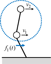
Figure 7. Story shear force f₁(t) in the first story and velocities of masses.

By substituting the condition d₁ − d_r1 = 0 (d_r1: residual deformation in the first story), derived from Eq. 27, into the expression of the total mechanical energy at the phase (B), the equation of the energy conservation between the phase (B) and (A) leads to

$\frac{1}{2}{m}_1{v}_1^2+\frac{1}{2}{m}_2{v}_2^2+\frac{1}{2}{k}_2{d}_2^2=\frac{1}{2}{k}_1{d}_{y1}^2+E_2^{(A)}.$ (28)

Rearrangement of Eq. 28 provides

$\frac{1}{2}{m}_1{v}_1^2+\frac{1}{2}{m}_2{v}_2^2=\frac{1}{2}{k}_1{d}_{y1}^2+E_2^{(A)}-\frac{1}{2}{k}_2{d}_2^2.$ (29)

Since the left-hand side of Eq. 29 is positive, the following inequality can be derived.

$0\le \frac{1}{2}{k}_2{d}_2^2\le \frac{1}{2}{k}_1{d}_{y1}^2+E_2^{(A)}\le \frac{1}{2}{k}_1{d}_{y1}^2+E_{2\max }^{(A)}.$ (30)

Let introduce the following quantity D.

$D=\frac{1}{2}{k}_1{d}_{y1}^2+E_{2\max }^{(A)}.$ (31)

Equation 29 and the positivity of $k_2{d}_2^2/2$ lead to the following relation (see Figure 8).

$\frac{1}{2}{m}_1{v}_1^2+\frac{1}{2}{m}_2{v}_2^2\le D.$ (32)

The tangential line of the ellipse $(m_1{v}_1^2/2)+(m_2{v}_2^2/2)=D$ at the point (v₁₀, v₂₀) can be expressed by

$\frac{v_{10}}{m_2}{v}_1+\frac{v_{20}}{m_1}{v}_2=\frac{2D}{m_1{m}_2}.$ (33)

Recalling P = m₁v₁ + m₂v₂, Eq. 33 provides

$\frac{v_{10}}{m_2}:\frac{v_{20}}{m_1}:\frac{2D}{m_1{m}_2}=m_1:m_2:P.$ (34)

The first proportionality relation in Eq. 34 leads to v₁₀ = v₂₀. The substitution of this relation into Eq. 33 and the other proportionality relation in Eq. 34 yields

$P=\sqrt{2\left(m_1+m_2\right)D}.$ (35)

FIGURE 8

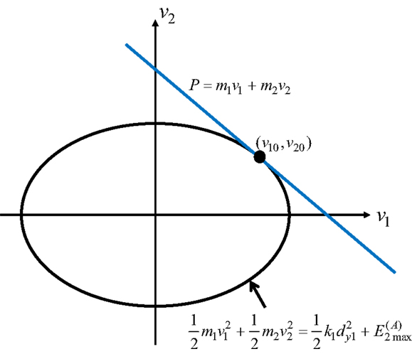
Figure 8. Tangential line of the ellipse $(m_1{v}_1^2/2)+(m_2{v}_2^2/2)=D$ at the point (v₁₀, v₂₀).

Finally, the upper bound ΔE_max of the input energy at the second impulse can be derived as

$\Delta E_{\max }=\frac{1}{2}\left(m_1+m_2\right)V^2+V\sqrt{2\left(m_1+m_2\right)\left(\frac{1}{2}{k}_1{d}_{y1}^2+E_{2\max }^{(A)}\right)}.$ (36)

This process employs the application of the convex model (Ben-Haim and Elishakoff, 1990). It may be interesting to note that the property (Eqs. 26 and 27) and the proof shown in this section can be extended to MDOF models.

On the other hand, it is meaningful to derive the lower bound of the input energy at the second impulse even approximately because the upper bound may not be a tight bound.

Assume that the total mechanical energy at the phase (A) is transformed into the kinetic energy of the first-story mass and that the second story does not have the strain energy and the kinetic energy. This assumption can be expressed by

$\frac{1}{2}{m}_1{v}_1^2=\frac{1}{2}{k}_1{d}_{y1}^2+E_2^{(A)}.$ (37)

Equation 37 leads to

$v_1=\sqrt{\frac{k_1}{m_1}{d}_{y1}^2+\frac{2E_2^{(A)}}{m_1}}$ (38)

$P=\sqrt{m_1\left(k_1{d}_{y1}^2+2E_2^{(A)}\right)}.$ (39)

Therefore, the approximate lower bound ΔE_min of the input energy at the second impulse can be derived as

$\Delta E_{\min }=\frac{1}{2}\left(m_1+m_2\right)V^2+V\sqrt{m_1\left(k_1{d}_{y1}^2+2E_2^{(A)}\right)}.$ (40)

Minimization of $E_2^{(D)}+k_2{d}_{y2}{d}_{p2}^{(2)}$ (Maximization of $E_2^{(D)}+k_2{d}_{y2}{d}_{p2}^{(2)}$ in Addition)

Since $E_2^{(D)}$ is the sum of the second-story strain energy and the second-story kinetic energy, the following relation is derived in the minimization of $E_2^{(D)}+k_2{d}_{y2}{d}_{p2}^{(2)}$.

$E_{2\min }^{(D)}=0$ (41)

$d_{p2\min }^{(2)}\doteq 0.$ (42)

On the other hand, the maximization of $E_2^{(D)}$ is difficult. Because the effect of the second impulse on the second-story interstory drift is small, it can be assumed that $d_{p2\max }^{(2)}\doteq 0$. Therefore, the following relations can be set approximately.

$E_{2\max }^{(D)}\doteq \frac{1}{2}{k}_2{d}_{y2}^2$ (43)

$d_{p2\max }^{(2)}\doteq 0.$ (44)

Upper Bound of Plastic Deformation in the First Story after the Second Impulse

Based on the results of Sections “Maximization of $E_2^{(A)}$,” “Maximization of ΔE (Minimization of ΔE in Addition),” and “Minimization of $E_2^{(D)}+k_2{d}_{y2}{d}_{p2}^{(2)}$ (Maximization of $E_2^{(D)}+k_2{d}_{y2}{d}_{p2}^{(2)}$ in Addition),” the upper bound of $d_{p1}^{(2)}$ can be derived by

$\begin{array}{l}\frac{d_{p1}^{(2)}}{d_{y1}}\le \frac{1}{k_1{d}_{y1}^2}\{\frac{\mu }{2\kappa }{k}_1{d}_{y1}^2+\frac{1}{2}\left(m_1+m_2\right)V^2+\sqrt{\left(m_1+m_2\right)\left(1+\frac{\mu }{\kappa }\right)k_1{d}_{y1}^2}V\}\\ =\frac{1}{k_1{d}_{y1}^2}\{\frac{\mu }{2\kappa }{k}_1{d}_{y1}^2+a^2\left(\frac{1}{2}{k}_1{d}_{y1}^2+\frac{1}{2}{k}_2{d}_{y2}^2\right)+a\sqrt{\left(1+\frac{\mu }{\kappa }\right)\left(k_1{d}_{y1}^2+k_2{d}_{y2}^2\right)k_1{d}_{y1}^2}\}(\mu >1)\end{array}$ (45a)

$\begin{array}{l}\frac{d_{p1}^{(2)}}{d_{y1}}\le \frac{1}{k_1{d}_{y1}^2}\{\frac{2{\mu }^2}{{\left(\mu +1\right)}^2\kappa }{k}_1{d}_{y1}^2+\frac{1}{2}\left(m_1+m_2\right)V^2+\sqrt{\left(m_1+m_2\right)\left(1+\frac{4{\mu }^2}{{\left(\mu +1\right)}^2\kappa }\right)k_1{d}_{y1}^2}V\}\\ =\frac{1}{k_1{d}_{y1}^2}\{\frac{2{\mu }^2}{{\left(\mu +1\right)}^2\kappa }{k}_1{d}_{y1}^2+a^2\left(\frac{1}{2}{k}_1{d}_{y1}^2+\frac{1}{2}{k}_2{d}_{y2}^2\right)+a\sqrt{\left(1+\frac{4{\mu }^2}{{\left(\mu +1\right)}^2\kappa }\right)\left(k_1{d}_{y1}^2+k_2{d}_{y2}^2\right)k_1{d}_{y1}^2}\}(\mu \le 1).\end{array}$ (45b)

In case of equal mass (μ = 1), equal story stiffness and equal yield interstory drift, Eq. 45b can be reduced to

$\frac{d_{p1}^{(2)}}{d_{y1}}\le a^2+2a+\frac{1}{2}\left(a=V/V_y\right).$ (46)

On the other hand, an approximate lower bound of $d_{p1}^{(2)}$ can be derived by substituting Eqs. 23 and 40 and 43 and 44 into Eq. 10.

$\begin{array}{l}\frac{d_{p1}^{(2)}}{d_{y1}}\ge \frac{1}{k_1{d}_{y1}^2}\{\frac{1}{2}\left(m_1+m_2\right)V^2+\sqrt{m_1{k}_1{d}_{y1}^2}V-\frac{1}{2}{k}_2{d}_{y2}^2\}\\ =\frac{1}{k_1{d}_{y1}^2}\{{\frac{a}{2}}^2\left(k_1{d}_{y1}^2+k_2{d}_{y2}^2\right)+a\sqrt{\frac{m_1}{m_1+m_2}\left(k_1{d}_{y1}^2+k_2{d}_{y2}^2\right)k_1{d}_{y1}^2}-\frac{1}{2}{k}_2{d}_{y2}^2\}.\end{array}$ (47)

In case of equal mass, equal story stiffness and equal yield interstory drift, Eq. 47 can be reduced to

$\frac{d_{p1}^{(2)}}{d_{y1}}\ge a^2+a-\frac{1}{2}\left(a=V/V_y\right).$ (48)

Numerical Examples of Critical Responses

Upper Bound of Critical Response

Consider a 2DOF model of equal mass (m₁ = m₂ = 1.0 × 10⁶ kg), equal story stiffness (k₁ = k₂ = 1.0 × 10⁸ N/m) and equal yield interstory drift (d_y1 = d_y2 = 0.1 m) subjected to the double impulse. The fundamental natural period is 1.02(s). For comparison, a reduced SDOF model as shown in Figure 9 is considered.

FIGURE 9

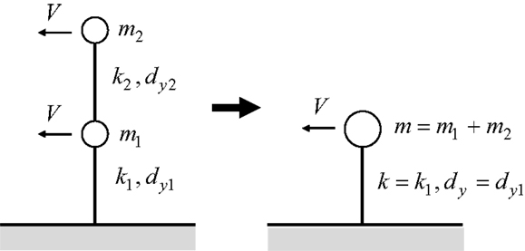
Figure 9. Transformation of 2DOF system into reduced SDOF system.

Figure 10 shows the maximum interstory drift after the first impulse in the first story in which the response of the SDOF system as shown in Figure 9 (also upper bound of 2DOF system) and the response under the corresponding one-cycle sinusoidal wave are also plotted. It should be remarked that the assumption of energy concentration into the first story provides the upper bound of the 2DOF system and this assumption is equivalent to the modeling into the reduced SDOF system. The response has been computed by using the Newmark-beta method. It can be observed that the upper bound of the 2DOF system can bound the actual critical response tightly. Although the response under the corresponding one-cycle sinusoidal wave is rather small in a larger input level, the correspondence up to about V/V_y = 3 may be meaningful from the practical view point.

FIGURE 10

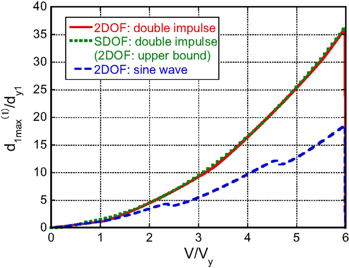
Figure 10. Maximum interstory drift after the first impulse in the first story together with the response of the SDOF system (also upper bound of 2DOF system) and the response under the corresponding one-cycle sinusoidal wave.

Figure 11 presents the maximum interstory drift after the second impulse in the first story in which the response of the SDOF system and the response under the corresponding one-cycle sinusoidal wave are also plotted. As stated in Figure 11, the correspondence up to about V/V_y = 3 may be meaningful from the practical view point. Figure 12 illustrates the critical plastic deformation after the second impulse in the first story and their upper and lower bounds (Eqs. 46 and 48) in which the upper bound of SDOF system and the response under the corresponding one-cycle sinusoidal wave are also plotted. It should be noted that, in the case of the elastic deformation in the first story after the first impulse (rather smaller input level: V/V_y ≤ 1.0 in this case), other expressions of the upper and lower bounds shown in Appendix 2 have to be employed.

FIGURE 11

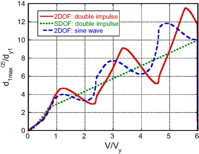
Figure 11. Maximum interstory drift after the second impulse in the first story.

FIGURE 12

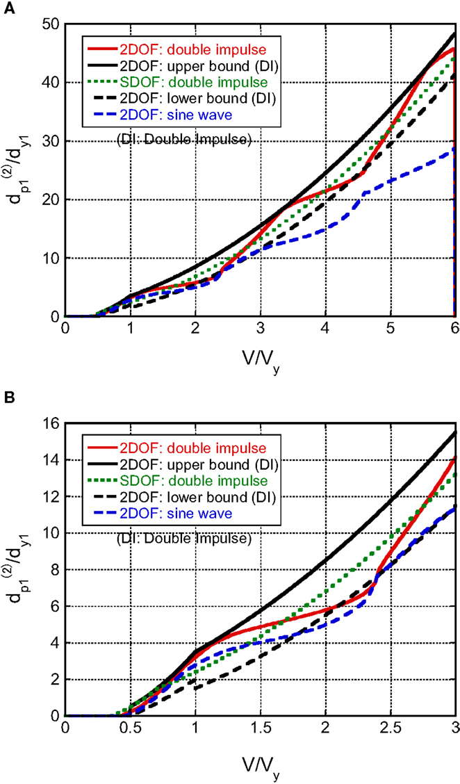
Figure 12. Critical plastic deformation after the second impulse in the first story and their upper and lower bounds together with the upper bound of SDOF system and the response under the corresponding one-cycle sinusoidal wave. (A) Comparison up to V/V_y = 6. (B) Magnified.

It can be seen that the actual critical plastic deformation after the second impulse in the first story corresponds fairly well with the response under the corresponding one-cycle sinusoidal wave up to about V/V_y = 3. Furthermore, the upper and lower bounds can bound the actual critical plastic deformation (although the lower bound is approximate due to the uncertain assumption of Eq. 44).

Figure 13 shows the critical timing t_0c of the second impulse with respect to the input level of the double impulse. This critical timing has been obtained using Eq. 27. For comparison, the critical timing for the corresponding SDOF model is also plotted. Consider that a structure is given, i.e., the parameters of the structure are specified. Then the critical timing t_0c can be found from Figure 13 (although the critical timing t_0c of a 2DOF model has to be evaluated numerically). The practical range of the period of pulses in near-fault ground motions may be 0.5–3 s. The fundamental natural period of most of buildings is in this range except very flexible high-rise buildings and base-isolated buildings. An important matter in the seismic design of structures for near-fault ground motions is to take into account the most unfavorable situation (resonant in elastic and elastic–plastic range). This can be justified because earthquake ground motions are highly uncertain (Takewaki, 2007).

FIGURE 13

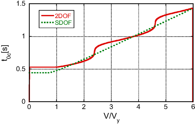
Figure 13. Critical timing of the second impulse with respect to the input level of double impulse.

It may be interesting to demonstrate the correspondence of the response to the double impulse with that to the sinusoidal wave in the time domain. The comparison of the time histories (first-story interstory drift and first-story restoring force) and the first-story restoring-force characteristic under the double impulse and the corresponding sinusoidal wave is shown in Appendix 3.

Input Level for Tight Upper Bound

Consider the same 2DOF model subjected to the double impulse with V/V_y = 1.11, 3.33, 5.55 at which the upper bound is close to the actual critical response in Figure 12. The increment 2.22 of input level has been analyzed by using the fundamental law in dynamics (Newton’s second law) (see Appendix 4). Figure 14 shows the time histories of the restoring forces in the first and second stories for the same 2DOF model subjected to the double impulse with V/V_y = 1.11, 3.33, 5.55. The critical timing t_0c is also shown in the figure captions.

FIGURE 14

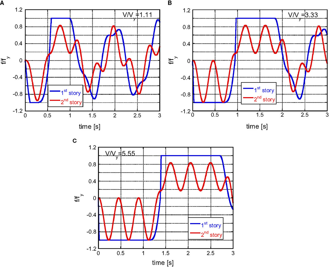
Figure 14. Time histories of the restoring forces in the first and second stories for the same 2DOF model subjected to the double impulse with V/V_y = 1.11, 3.33, 5.55. (A) V/V_y = 1.11 (t_0c = 0.535 [s]). (B) V/V_y = 3.33 (t_0c = 0.946 [s]). (C) V/V_y = 5.55 (t_0c = 1.384 [s]).

Figure 15 presents the deformation mode and velocity at the phase (A). Figure 16 illustrates the time histories of the restoring forces in the first and second stories starting from the phase (A) (only the first impulse is given: V/V_y = 1.11, 3.33, 5.55). Figure 17 shows the velocity (first-story mass)-velocity (second-story mass) plane for variable motion of masses attaining the maximum sum of momenta (tangential line) by the convex model and the actual motion of masses starting from the phase (A) (only the first impulse is given: V/V_y = 1.11, 3.33, 5.55). It can be observed from Figure 17 that the actual motion of masses passes through the solution derived by the convex model.

FIGURE 15

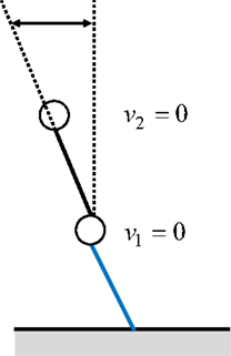
Figure 15. Deformation mode and velocity at the phase (A) (upper bound case).

FIGURE 16

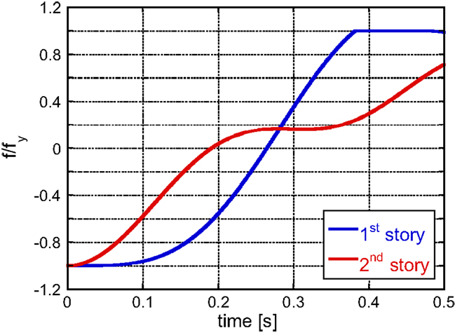
Figure 16. Time histories of the restoring forces in the first and second stories starting from the phase (A).

FIGURE 17

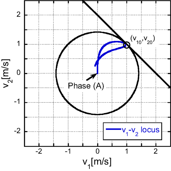
Figure 17. Velocity (first-story mass)-Velocity (second-story mass) plane for variable motion of masses attaining the maximum sum of momenta (tangential line) by the convex model and the actual motion of masses starting from the phase (A) (only the first impulse is given).

Input Level for Loose Upper Bound

Consider the same 2DOF model subjected to the double impulse with V/V_y = 2.22, 4.44 at which the upper bound is far from the actual critical response in Figure 12 (the lower bound is close to the actual critical one). As stated in Section 6.2, the increment 2.22 of input level has been analyzed by using the fundamental law in dynamics (Newton’s second law). Figure 18 shows the time histories of the restoring forces in the first and second stories for the same 2DOF model subjected to the double impulse with V/V_y = 2.22, 4.44 In this example, $d_{p2}^{(2)}$ exists which was discussed in Eq. 8. The critical timing t_0c is also shown in the figure captions.

FIGURE 18

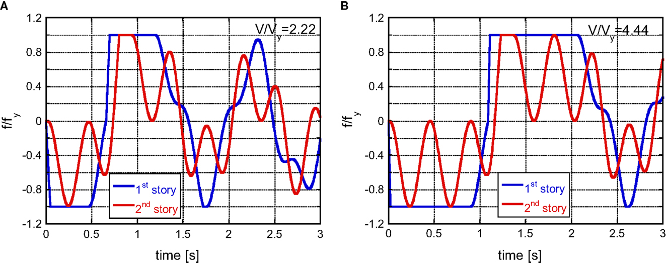
Figure 18. Time histories of the restoring forces in the first and second stories for the same 2DOF model subjected to the double impulse with V/V_y = 2.22, 4.44. (A) V/V_y = 2.22 (t_0c = 0.658 [s]). (B) V/V_y = 4.44 (t_0c = 1.089 [s]).

Figure 19 presents the deformation mode and velocity at the phase (A). Figure 20 illustrates the time histories of the restoring forces in the first and second stories starting from the phase (A) (only the first impulse is given: V/V_y = 2.22, 4.44). Figure 21 shows the velocity (first-story mass)-velocity (second-story mass) plane for variable motion of masses bounded by shrinked circle and the actual motion of masses starting from the phase (A) (only the first impulse is given: V/V_y = 2.22, 4.44). It can be observed from Figure 21 that the actual motion of masses is far from the solution derived by the convex model.

FIGURE 19

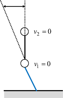
Figure 19. Deformation mode and velocity at the phase (A) (lower bound case).

FIGURE 20

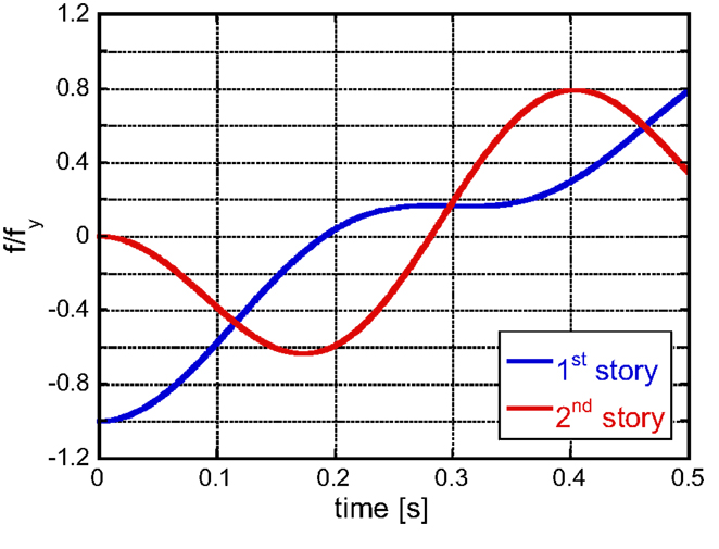
Figure 20. Time histories of the restoring forces in the first and second stories starting from the phase (A).

FIGURE 21

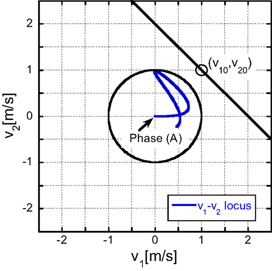
Figure 21. Velocity (first-story mass)–Velocity (second-story mass) plane for variable motion of masses bounded by shrinked circle and the actual motion of masses starting from the phase (A) (only the first impulse is given).

Verification of Criticality

In order to demonstrate the criticality of the timing of the second impulse defined by Eq. 27, a parametric analysis for the varied timing of the second impulse has been performed. Figure 22 shows the plot of $d_{p1}^{(2)}/d_{y1}$ with respect to the timing of the second impulse. The restoring force in the first story at the second impulse is also plotted for reference. It can be seen that the criterion of the zero restoring force in the first story defined by Eq. 27 certainly maximizes $d_{p1}^{(2)}/d_{y1}$ in addition to maximizing the input energy at the second impulse.

FIGURE 22

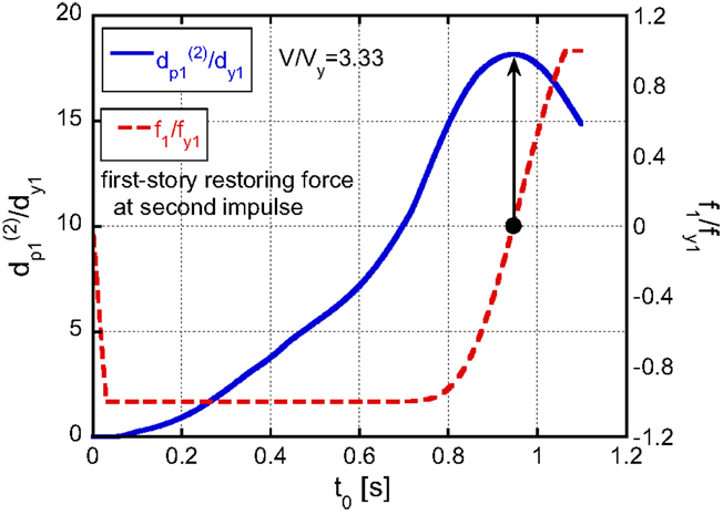
Figure 22. Plot of $d_{p1}^{(2)}$ and f₁/f_y1 (restoring force in the first story at the second impulse) with respect to the timing of the second impulse.

Application to Recorded Ground Motion

To investigate the applicability of the present theory to actual recorded pulse-type ground motions, a comparison of the proposed upper bound with the corresponding response to a recorded ground motion is presented.

Consider the Rinaldi station fault-normal component during the Northridge earthquake in 1994 as a representative pulse-type ground motion. The structural model is the same as in Section “Upper Bound of Critical Response” (equal mass, equal stiffness, and equal yield interstory drift in each story). Since the ground motion is fixed (V and t₀ are fixed), the structural model parameters are varied, i.e., V_y (specifically k₁ = k₂ and d_y1 = d_y2) is varied. Figure 23A illustrates the modeling of a part of the recorded ground motion acceleration into a one-cycle sinusoidal input. Figure 23B shows the maximum amplitude of plastic deformation for the recorded ground motion by time-history response analysis and the proposed upper bound for the corresponding double impulse. As stated before, since the initial velocity V is determined in Figure 23A, V_y is changed here. This procedure is similar to the well-known elastic–plastic response spectrum developed in 1960–1970. The solid line is obtained by changing V_y for the specified V using the proposed method for the upper bound to the double impulse and the dotted line is drawn by conducting the elastic–plastic time-history response analysis on each model with varied V_y under the recorded ground motion. It can be observed that the result by the proposed method is a fairly good upper-bound approximate of the result to the recorded pulse-type ground motion.

FIGURE 23

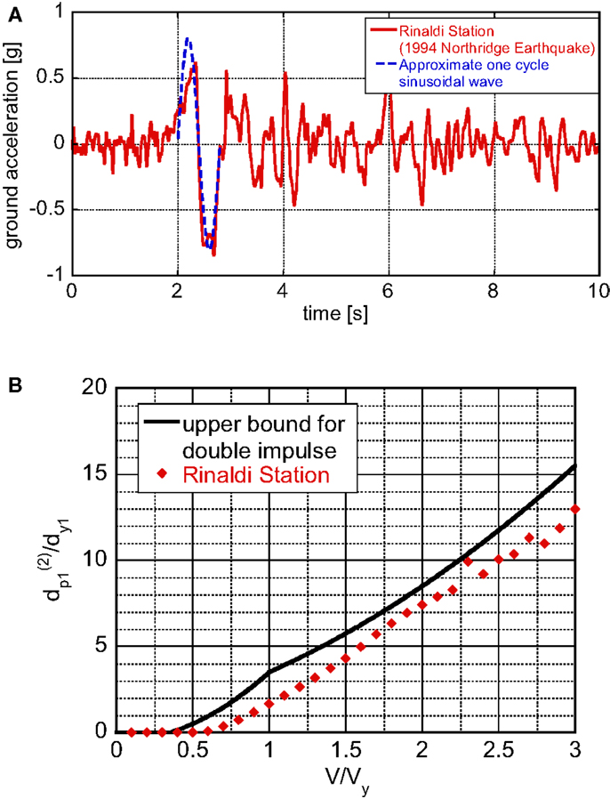
Figure 23. Applicability to recorded ground motion: (A) Modeling of part of pulse-type recorded ground motion (Rinaldi station fault-normal component during the Northridge earthquake in 1994) into the corresponding one-cycle sinusoidal input: (B) Maximum amplitude of plastic deformation for the recorded ground motion and the proposed upper bound for the corresponding double impulse.

Conclusion

The conclusions may be summarized as follows:

(1) The double impulse has been introduced as a substitute of the fling-step near-fault ground motion and a critical elastic–plastic response of a 2DOF building structure under the “critical double impulse” has been evaluated. The critical excitation problem is such that the velocity amplitude of the double impulse is fixed and the interval of the double impulse is the variable. Since only the free-vibration appears under such double impulse, the energy balance approach plays an important and essential role in the direct derivation of the complicated elastic–plastic critical response.

(2) The criticality is characterized by the timing of the second impulse at the zero story shear force in the first story. This timing guarantees the maximum energy input by the second impulse that causes the maximum plastic deformation after the second impulse in the first story. This critical timing also coincides with the state in which the sum of the momenta attains the maximum. This property can be extended to MDOF models.

(3) Because the response of 2DOF elastic–plastic building structures is quite complicated due to the phase difference between two masses compared to SDOF models for which a closed-form critical response can be derived, the upper bound of the critical response has been introduced. The upper bound has been derived by using the convex model partially.

(4) As for the maximum interstory drift in the first story after the first impulse, the proposed upper bound is close to the actual maximum response. Although the response to the corresponding sine wave is rather smaller than that to the double impulse in the larger input level, the practical interest is up to about the input level V/V_y = 3.

(5) As for the plastic deformation after the second impulse in the first story, the proposed upper bound certainly bounds the actual plastic deformation and the devised lower bound approximately circumvents the actual response from the lower side. As stated above, the practical interest is up to about the input level V/V_y = 3.

(6) The actual critical response of plastic deformation after the second impulse in the first story is close to the upper or lower bound at discrete input levels. Such discrete level has been analyzed by using the fundamental law in dynamics (Newton’s second law).

(7) It has been demonstrated that the proposed method using the double impulse and the upper bound is applicable to actual recorded pulse-type ground motions within a reasonable accuracy.

In this paper, the case has been treated where the second story does not go into the plastic range after the first impulse. As stated before, this case is often the case when the condition, Eq. 17, is satisfied. The other case could be discussed in the future if necessary. As for damping, it is well recognized that the viscous damping is not effective for impulsive ground motions like near-fault ground motions. The effect in an elastic SDOF model is shown in Appendix 5. The effect of damping on the conservativeness of the proposed upper bound should be discussed in the future.

Author Contributions

RT carried out the theoretical and numerical analysis. KK helped the numerical analysis. IT supervised the theoretical analysis and organized the research group. All authors read and approved the final manuscript.

Conflict of Interest Statement

The authors declare that the research was conducted in the absence of any commercial or financial relationships that could be construed as a potential conflict of interest.

Funding

Part of the present work is supported by the Grant-in-Aid for Scientific Research of Japan Society for the Promotion of Science (No.15H04079) and the 2013-MEXT-Supported Program for the Strategic Research Foundation at Private Universities in Japan. These supports are greatly appreciated.

References

Abbas, A. M., and Manohar, C. S. (2002). Investigations into critical earthquake load models within deterministic and probabilistic frameworks. Earthquake Eng. Struct. Dyn. 31, 813–832. doi: 10.1002/eqe.124.abs

CrossRef Full Text | Google Scholar

Alavi, B., and Krawinkler, H. (2004). Behaviour of moment resisting frame structures subjected to near-fault ground motions. Earthquake Eng. Struct. Dyn. 33, 687–706. doi:10.1002/eqe.369

CrossRef Full Text | Google Scholar

Ben-Haim, Y., Chen, G., and Soong, T. T. (1996). Maximum structural response using convex models. J. Eng. Mech. 122, 325–333. doi:10.1061/(ASCE)0733-9429(1996)122:6(325)

CrossRef Full Text | Google Scholar

Ben-Haim, Y., and Elishakoff, I. (1990). Convex Models of Uncertainty in Applied Mechanics. Amsterdam: Elsevier.

Google Scholar

Bertero, V. V., Mahin, S. A., and Herrera, R. A. (1978). Aseismic design implications of near-fault San Fernando earthquake records. Earthquake Eng. Struct. Dyn. 6, 31–42. doi:10.1002/eqe.4290060105

CrossRef Full Text | Google Scholar

Bray, J. D., and Rodriguez-Marek, A. (2004). Characterization of forward-directivity ground motions in the near-fault region. Soil Dyn. Earthquake Eng. 24, 815–828. doi:10.1016/j.soildyn.2004.05.001

CrossRef Full Text | Google Scholar

Caughey, T. K. (1960a). Sinusoidal excitation of a system with bilinear hysteresis. J. Appl. Mech. 27, 640–643. doi:10.1115/1.3644077

CrossRef Full Text | Google Scholar

Caughey, T. K. (1960b). Random excitation of a system with bilinear hysteresis. J. Appl. Mech. 27, 649–652. doi:10.1115/1.3644077

CrossRef Full Text | Google Scholar

Drenick, R. F. (1970). Model-free design of aseismic structures. J. Eng. Mech. Div. 96, 483–493.

Google Scholar

Hall, J. F., Heaton, T. H., Halling, M. W., and Wald, D. J. (1995). Near-source ground motion and its effects on flexible buildings. Earthuake Spectra 11, 569–605. doi:10.1193/1.1585828

CrossRef Full Text | Google Scholar

Hayden, C. P., Bray, J. D., and Abrahamson, N. A. (2014). Selection of near-fault pulse motions. J. Geotech. Geoenviron. Eng. 140. doi:10.1061/(ASCE)GT.1943-5606.0001129

CrossRef Full Text | Google Scholar

Iwan, W. D. (1961). The Dynamic Response of Bilinear Hysteretic Systems. Ph.D. thesis, California Institute of Technology, Pasadena.

Google Scholar

Iwan, W. D. (1965a). “The dynamic response of the one-degree-of-freedom bilinear hysteretic system,” in Proceedings of the Third World Conference on Earthquake Engineering, New Zealand.

Google Scholar

Iwan, W. D. (1965b). The steady-state response of a two-degree-of-freedom bilinear hysteretic system. J. Appl. Mech. 32, 151–156. doi:10.1115/1.3625711

CrossRef Full Text | Google Scholar

Iwan, W. D. (1997). Drift spectrum: measure of demand for earthquake ground motions. J. Struct. Eng. 123, 397–404. doi:10.1061/(ASCE)0733-9445(1997)123:4(397)

CrossRef Full Text | Google Scholar

Kalkan, E., and Kunnath, S. K. (2006). Effects of fling step and forward directivity on seismic response of buildings. Earthquake Spectra 22, 367–390. doi:10.1193/1.2192560

CrossRef Full Text | Google Scholar

Kalkan, E., and Kunnath, S. K. (2007). Effective cyclic energy as a measure of seismic demand. J. Earthquake Eng. 11, 725–751. doi:10.1080/13632460601033827

CrossRef Full Text | Google Scholar

Khaloo, A. R., Khosravi, H., and Hamidi Jamnani, H. (2015). Nonlinear interstory drift contours for idealized forward directivity pulses using “modified fish-bone” models. Adv. Struct. Eng 18, 603–627. doi:10.1260/1369-4332.18.5.603

CrossRef Full Text | Google Scholar

Kojima, K., Fujita, K., and Takewaki, I. (2015). Critical double impulse input and bound of earthquake input energy to building structure. Front. Built Environ. 1:5. doi:10.3389/fbuil.2015.00005

CrossRef Full Text | Google Scholar

Kojima, K., and Takewaki, I. (2015a). Critical earthquake response of elastic-plastic structures under near-fault ground motions (part 1: fling-step input). Front. Built Environ. 1:12. doi:10.3389/fbuil.2015.00012

CrossRef Full Text | Google Scholar

Kojima, K., and Takewaki, I. (2015b). Critical earthquake response of elastic-plastic structures under near-fault ground motions (part 2: forward-directivity input). Front. Built Environ. 1:13. doi:10.3389/fbuil.2015.00012

CrossRef Full Text | Google Scholar

Kojima, K., and Takewaki, I. (2015c). Critical input and response of elastic-plastic structures under long-duration earthquake ground motions. Front. Built Environ. 1:15. doi:10.3389/fbuil.2015.00012

CrossRef Full Text | Google Scholar

Liu, C.-S. (2000). The steady loops of SDOF perfectly elastoplastic structures under sinusoidal loadings. J. Marine Sci. Technol. 8, 50–60.

Google Scholar

Makris, N., and Black, C. J. (2004). Dimensional analysis of rigid-plastic and elastoplastic structures under pulse-type excitations. J. Eng. Mech. 130, 1006–1018. doi:10.1061/(ASCE)0733-9399(2004)130:9(1006)

CrossRef Full Text | Google Scholar

Mavroeidis, G. P., Dong, G., and Papageorgiou, A. S. (2004). Near-fault ground motions, and the response of elastic and inelastic single-degree-freedom (SDOF) systems. Earthquake Eng. Struct. Dyn. 33, 1023–1049. doi:10.1002/eqe.391

CrossRef Full Text | Google Scholar

Mavroeidis, G. P., and Papageorgiou, A. S. (2003). A mathematical representation of near-fault ground motions. Bull. Seism. Soc. Am. 93, 1099–1131. doi:10.1785/0120020100

CrossRef Full Text | Google Scholar

Minami, H., and Hayashi, Y. (2013). Response characteristics evaluation of elastic shear bean for pulse waves. J. Struct. Construct. Eng. 685, 453–461. doi:10.3130/aijs.78.453

CrossRef Full Text | Google Scholar

Moustafa, A., Ueno, K., and Takewaki, I. (2010). Critical earthquake loads for SDOF inelastic structures considering evolution of seismic waves. Earthquakes Struct. 1, 147–162. doi:10.12989/eas.2010.1.2.147

CrossRef Full Text | Google Scholar

Mukhopadhyay, S., and Gupta, V. K. (2013a). Directivity pulses in near-fault ground motions – I: identification, extraction and modeling. Soil Dyn. Earthquake Eng. 50, 1–15. doi:10.1016/j.soildyn.2013.02.017

CrossRef Full Text | Google Scholar

Mukhopadhyay, S., and Gupta, V. K. (2013b). Directivity pulses in near-fault ground motions – II: estimation of pulse parameters. Soil Dyn. Earthquake Eng. 50, 38–52. doi:10.1016/j.soildyn.2013.02.017

CrossRef Full Text | Google Scholar

Roberts, J. B., and Spanos, P. D. (1990). Random Vibration and Statistical Linearization. New York: Wiley.

Google Scholar

Rupakhety, R., and Sigbjörnsson, R. (2011). Can simple pulses adequately represent near-fault ground motions? J. Earthquake Eng. 15, 1260–1272. doi:10.1080/13632469.2011.565863

CrossRef Full Text | Google Scholar

Sasani, M., and Bertero, V. V. (2000). “Importance of severe pulse-type ground motions in performance-based engineering: historical and critical review,” in Proceedings of the Twelfth World Conference on Earthquake Engineering (Auckland).

Google Scholar

Singh, J. P. (1984). “Characteristics of near-field strong ground motion and their importance in building design,” in Proceeding of Critical Aspects of Earthquake Ground Motion and Building Damage Potential (ATC-10-1) (Palo Alto, CA: Applied Technology Council), 23–42.

Google Scholar

Takewaki, I. (1996). Design-oriented approximate bound of inelastic responses of a structure under seismic loading. Comput. Struct. 61, 431–440. doi:10.1016/0045-7949(96)00086-7

CrossRef Full Text | Google Scholar

Takewaki, I. (1997). Design-oriented ductility bound of a plane frame under seismic loading. J. Vib. Contr. 3, 411–434. doi:10.1177/107754639700300404

CrossRef Full Text | Google Scholar

Takewaki, I. (2002). Robust building stiffness design for variable critical excitations. J. Struct. Eng. 128, 1565–1574. doi:10.1061/(ASCE)0733-9445(2002)128:12(1565)

CrossRef Full Text | Google Scholar

Takewaki, I. (2007). Critical Excitation Methods in Earthquake Engineering, 2nd Edn. Oxford: Elsevier.

Google Scholar

Takewaki, I., Moustafa, A., and Fujita, K. (2012). Improving the Earthquake Resilience of Buildings: The Worst Case Approach. London: Springer.

Google Scholar

Takewaki, I., and Tsujimoto, H. (2011). Scaling of design earthquake ground motions for tall buildings based on drift and input energy demands. Earthquakes Struct. 2, 171–187. doi:10.12989/eas.2011.2.2.171

CrossRef Full Text | Google Scholar

Vafaei, D., and Eskandari, R. (2015). Seismic response of mega buckling-restrained braces subjected to fling-step and forward-directivity near-fault ground motions. Struct. Des. Tall Spec. Build. 24, 672–686. doi:10.1002/tal.1205

CrossRef Full Text | Google Scholar

Vassiliou, M. F., Tsiavos, A., and Stojadinovic, B. (2013). Dynamics of inelastic base-isolated structures subjected to analytical pulse ground motions. Earthquake Eng. Struct. Dyn. 42, 2043–2060. doi:10.1002/eqe.2311

CrossRef Full Text | Google Scholar

Xu, Z., Agrawal, A. K., He, W.-L., and Tan, P. (2007). Performance of passive energy dissipation systems during near-field ground motion type pulses. Eng. Struct. 29, 224–236. doi:10.1016/j.engstruct.2006.04.020

CrossRef Full Text | Google Scholar

Yamamoto, K., Fujita, K., and Takewaki, I. (2011). Instantaneous earthquake input energy and sensitivity in base-isolated building. Struct. Des. Tall Spec. Build. 20, 631–648. doi:10.1002/tal.539

CrossRef Full Text | Google Scholar

Yang, D., and Zhou, J. (2014). A stochastic model and synthesis for near-fault impulsive ground motions. Earthquake Eng. Struct. Dyn. 44, 243–264. doi:10.1002/eqe.2468

CrossRef Full Text | Google Scholar

Zhai, C., Chang, Z., Li, S., Chen, Z.-Q., and Xie, L. (2013). Quantitative identification of near-fault pulse-like ground motions based on energy. Bull. Seism. Soc. Am. 103, 2591–2603. doi:10.1785/0120120320

CrossRef Full Text | Google Scholar

Appendix 1

Adjustment of Input Level of Double Impulse and Corresponding One-Cycle Sinusoidal Wave

The adjustment of the input level of the double impulse and the corresponding one-cycle sinusoidal wave is achieved based on the equivalence of the maximum value of the Fourier amplitude. Figure A1 shows an example.

FIGURE A1

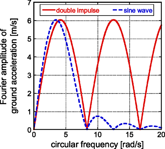
Figure A1. Adjustment of input level of double impulse and the corresponding one-cycle sinusoidal wave based on Fourier amplitude equivalence.

Appendix 2

Upper Bound and Lower Bound of Plastic Deformation in the First Story after the Second Impulse (Case of the Elastic Response in the First Story after the First Impulse)

In the case of the elastic response in the first story after the first impulse, another formulation is necessary. At the phase (D), the energy balance can be expressed by

$\frac{1}{2}\left(m_1+m_2\right)V^2+\Delta E=\frac{1}{2}{k}_1{d}_{y1}^2+k_1{d}_{y1}{d}_{p1}^{(2)}+E_2^{(D)}+k_2{d}_{y2}{d}_{p2}$ (A1)

Eq. A1 corresponds to Eq. 9 for the case of the plastic response in the first story after the first impulse and can be rearranged into

$\frac{d_{p1}^{(2)}}{d_{y1}}=\frac{1}{k_1{d}_{y1}^2}\left\{\frac{1}{2}\left(m_1+m_2\right)V^2+\Delta E-\left(E_2^{(D)}+k_2{d}_{y2}{d}_{p2}^{(2)}\right)\right\}-\frac{1}{2}$ (A2)

Upper Bound

In Eq. A2, the upper bound of the plastic deformation $d_{p1}^{(2)}$ of the first story after the second impulse can be derived by maximizing $\Delta E$ and minimizing $E_2^{(D)}$ and $d_{p2}^{(2)}$. Then, the upper bound can be obtained from the following setting.

$\Delta E_{\max }=\frac{3}{2}\left(m_1+m_2\right)V^2$ (A3)

$E_{2\min }^{(D)}=0$ (A4)

$d_{p2\min }^{(2)}\doteq 0$ (A5)

In this case, the upper bound of the plastic deformation in the first story after the second impulse can be expressed as

$\frac{d_{p1}^{(2)}}{d_{y1}}\le \frac{1}{k_1{d}_{y1}^2}\left\{2a^2\left(k_1{d}_{y1}^2+k_2{d}_{y2}^2\right)\right\}-\frac{1}{2}$ (A6)

For the model of equal mass, equal story stiffness and equal yield interstory drift, Eq. A6 can be reduced to

$\frac{d_{p1}^{(2)}}{d_{y1}}\le 4a^2-\frac{1}{2}$ (A7)

Lower Bound

In Eq. A2, the lower bound of the plastic deformation $d_{p1}^{(2)}$ of the first story after the second impulse can be derived by minimizing ΔE and maximizing $E_2^{(D)}$ and $d_{p2}^{(2)}$. It is often the case that the second story is in the elastic range even after the second impulse in a rather smaller input level considered here. Then, the lower bound can be obtained from the following setting.

$\Delta E_{\min }=\frac{1}{2}\left(m_1+m_2\right)V^2+V\sqrt{m_1{k}_1{d}_{y1}^2}$ (A8)

$E_{2\max }^{(D)}\doteq \frac{1}{2}{k}_2{d}_{y2}^2$ (A9)

$d_{p2\max }^{(2)}\doteq 0$ (A10)

In this case, the lower bound of the plastic deformation in the first story after the second impulse can be expressed as

$\begin{array}{ll}\frac{d_{p1}^{(2)}}{d_{y1}}& \ge \frac{1}{k_1{d}_{y1}^2}\{a^2\left(k_1{d}_{y1}^2+k_2{d}_{y2}^2\right)+a\sqrt{\frac{m_1}{m_1+m_2}\left(k_1{d}_{y1}^2+k_2{d}_{y2}^2\right)k_1{d}_{y1}^2}-\frac{1}{2}{k}_2{d}_{y2}^2\}-\frac{1}{2}\end{array}$ (A11)

For the model of equal mass, equal story stiffness and equal yield interstory drift, Eq. A6 can be reduced to

$\frac{d_{p1}^{(2)}}{d_{y1}}\ge 2a^2+a-1$ (A12)

Appendix 3

Comparison of Time Histories Under Double Impulse and Sinusoidal Wave

Consider the 2DOF model of equal mass, equal story stiffness, and equal yield interstory drift as treated above. Figures A2 and A3 show the comparison of the time histories (first-story interstory drift and first-story restoring force) and the first-story restoring-force characteristic, respectively, under the double impulse and the corresponding sinusoidal wave.

FIGURE A2

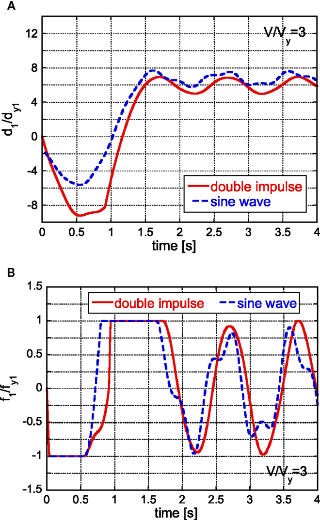
Figure A2. Comparison of time histories of the first-story interstory drift and the first-story restoring force under the double impulse and the corresponding sinusoidal wave. (A) First-story interstory drift. (B) First-story restoring force.

FIGURE A3

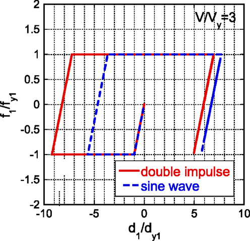
Figure A3. Comparison of first-story restoring-force characteristic under the double impulse and the corresponding sinusoidal wave.

Appendix 4

Input Level of Double Impulse for Characterizing Critical Response Close to Upper or Lower Bound

In Figure 12, the actual critical response of plastic deformation after the second impulse in the first story is close to the upper or lower bound at discrete input levels. Such discrete input level is investigated here.

Consider the deformation phase shown in Figure 15. At the phase (A), both masses are at rest and have zero velocities. In this case, the impulse (force × time interval) due to the restoring force in the first story is equal to the change of the sum of momenta at the input level V = V₁ (see Figure A4).

$\left(m_1+m_2\right)V_1={\displaystyle \underset{0}{\overset{t_1}{\int }}{f}_1\left(t\right)dt}$ (A13)

where t₁ is the time at the phase (A). The restoring forces after the first impulse are treated as positive values in this section. For another input level V = V₁ + ΔV, a similar relation holds (see Figure A4).

$\left(m_1+m_2\right)(V_1+\Delta V)={\displaystyle \underset{0}{\overset{t_1+\Delta t}{\int }}{f}_1\left(t\right)dt}$ (A14)

where t₁ + Δt is the time at the phase (A) for the input level V = V₁ + ΔV. Since the time up to the first yielding of the first story is quite short, the following relation can be drawn approximately by subtracting Eq. A13 from Eq. A14.

$\left(m_1+m_2\right)\Delta V={\displaystyle \underset{t_1}{\overset{t_1+\Delta t}{\int }}{f}_1\left(t\right)dt}$ (A15)

FIGURE A4

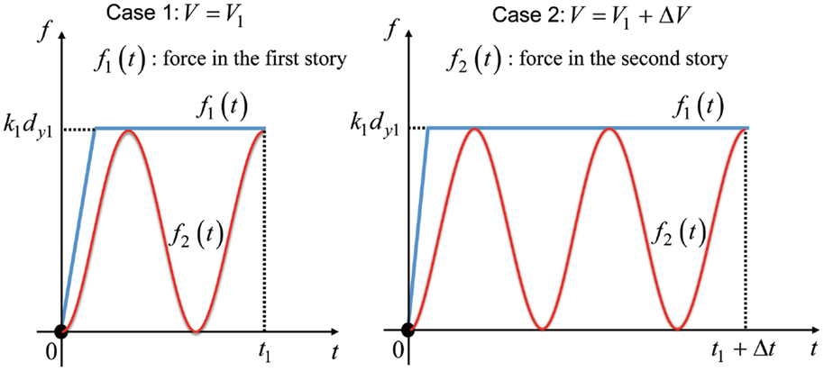
Figure A4. Time histories of the restoring forces in the first and second stories up to the phase (A).

Because Δt = 2π/ω is the period of the second story defined by Eq. 14a (circular frequency ω) and f₁ = k₁d_y1, the following relation holds.

$\left(m_1+m_2\right)\Delta V=2\pi \sqrt{\frac{m_1{m}_2}{\left(m_1+m_2\right)k_2}}{k}_1{d}_{y1}$ (A16)

Normalizing Eq. A16 by $V_y=\sqrt{(k_1{d}_{y1}^2+k_2{d}_{y2}^2)/(m_1+m_2)}$ defined in Eq. 3, the discrete input level ΔV is derived as

$\frac{\Delta V}{V_y}=2\pi \frac{\sqrt{m_1{m}_2}}{m_1+m_2}\frac{k_1{d}_{y1}}{\sqrt{k_2\left(k_1{d}_{y1}^2+k_2{d}_{y2}^2\right)}}$ (A17)

In the 2DOF model of equal mass, equal story stiffness and equal yield interstory drift as treated above, the following result is obtained.

$\Delta V/V_y=2.22$ (A18)

This certainly corresponds to the discrete interval of input level observed in Figures 12 and 13.

Appendix 5

Effect of Viscous Damping

In order to investigate the effect of viscous damping on the response under impulsive loading, consider an elastic damped single degree-of-freedom model. Let ω₁, h denote the undamped natural circular frequency and the damping ratio. When the model is subjected to an initial velocity v₀ (0 initial displacement), the displacement response can be expressed as

$u=\frac{v_0}{\sqrt{1-h^2}{\omega }_1}{e}^{-h{\omega }_{1}t}\sin \sqrt{1-h^2}{\omega }_{1}t$ (A19)

When we consider one-cycle sinusoidal input corresponding to the double impulse, the phase ω₁t of the first peak corresponds to π/2 and the phase of the second peak corresponds to 3π/2. In case of the damping ratio h = 0.02, the ratio $e^{-h{\omega }_{1}t}/\sqrt{1-h^2}$ of the displacement amplitude of the damped model to that of the undamped model is obtained as follows:

$e^{-h{\omega }_{1}t}/\sqrt{1-h^2}=0.\text{97\hspace{0.17em}for\hspace{0.17em}}{\omega }_{1}t=\pi /2$ (A20a)

$e^{-h{\omega }_{1}t}/\sqrt{1-h^2}=0.91\text{\hspace{0.17em}for\hspace{0.17em}}{\omega }_{1}t=3\pi /2$ (A20b)

This indicates that the damping effect is only 3% for the first peak and 9% for the second peak. It can be said that the viscous damping effect may be small in case of impulsive loading.