Estimation of Wind-Induced Pressures on a Low-Rise Building Using Quasi-Steady Theory

Introduction

In many wind tunnel measurements, building surface pressures, Δp, are related to the mean velocity, $\overline{V}$, through standard (or typical) pressure coefficients, C_p,t,

$\mathrm{\Delta }p=\frac{1}{2}\mathrm{\rho }{\overline{V}}^2{C}_{\text{p,t}}$ (1)

where ρ denotes the air density and Δp denotes the difference between the surface pressure, p, and ambient static pressure, p₀, i.e., Δp = p − p₀. Often, pressure coefficients are measured directly with the mean velocity obtained via a Pitot-static tube placed in a low turbulence region away from the building model (e.g., Ho et al., 2005). This allows straightforward calibration for accurate measurements, but implies that pressure coefficients must be re-referenced using velocities measured separately (e.g., Ho et al., 2005). By contrast, the quasi-steady (QS) theory assumes that the instantaneous surface pressures are a multiplication of the instantaneous dynamic pressure, 0.5ρV², and the instantaneous pressure coefficient, C_p,inst, i.e.,

$\mathrm{\Delta }p=\frac{1}{2}\mathrm{\rho }{V}^2{C}_{\text{p,inst}}$ (2)

where V is the magnitude of velocity, which is formed by its components in longitudinal, u, transverse, v, and vertical, w, directions, i.e.,

$V^2=u^2+v^2+w^2$ (3)

The corresponding azimuth, θ, and elevation, β, angles of the wind vector are defined as

$\mathrm{\theta }={\tan }^{-1}\left(\frac{v}{u}\right),\mathrm{\beta }={\tan }^{-1}\left(\frac{w}{\sqrt{u^2+v^2}}\right)$ (4a,b)

One of the advantages in considering the QS formulation in Eq. 2 is that the instantaneous building surface pressure is separated into the contribution from the instantaneous dynamic pressure and the contribution from other aerodynamic effects, such as body-generated turbulence, embedded in C_p,inst.

The variation of C_p,inst plays a crucial role in QS theory in estimating surface pressures based on the formulation in Eq. 2. For instance, some of the earlier research applied QS theory (e.g., Kawai, 1983; Letchford et al., 1993) by considering the effects of wind azimuth variations, which have been shown to affect the variance of C_p,inst in addition to wind speed variations. To model the effects of wind direction variations, linear functions for C_p,inst(θ) are often used for simplicity. In particular, the slope and intercept of the linear function are evaluated from the mean values of the typical pressure coefficients such that

$C_{\text{p,inst}}\left(\mathrm{\theta }\right)={\overline{C}}_{\text{p,t}}\left(\overline{\mathrm{\theta }}\right)+\left(\mathrm{\theta }-\overline{\mathrm{\theta }}\right)\left(d{\overline{C}}_{\text{p,t}}/d\overline{\mathrm{\theta }}\right),$

where the overbar represents time-mean values. Richards et al. (1995) proposed treating the wind azimuth effects non-linearly by representing C_p,inst(θ) as a Fourier series with experimentally determined coefficients. These authors found that the instantaneous pressure coefficients are generally different than the typical mean pressure coefficients because of smoothing effects caused by the averaging of the mean wind direction in the mean coefficients. This has the effective of lowering the magnitudes of the peak values (Richards et al., 1995). Banks and Meroney (2001) later compared the conditionally averaged instantaneous pressure coefficients, E[C_p,inst|θ], with a non-linear QS model similar to that proposed by Richards et al. (1995). They found that their non-linear model worked well for point pressures near the roof corner of a low-rise building, except for cases when the mean wind direction is approximately perpendicular to the roof edge.

Cook (1990) mentioned that the most comprehensive way to apply QS theory is to include both wind azimuth and elevation-angle variations in the instantaneous pressure coefficients, C_p,inst(θ, β). The effects of wind elevation angle have been investigated by several researchers (e.g., Letchford and Marwood, 1997; Sharma and Richards, 1999). In these experimental studies, building models were tilted so that the surface pressures were altered by winds at different mean elevation angles. Richards and Hoxey (2004) used a similar approach in their full-scale field study of roof point pressures by tilting the 6-meter-tall Silsoe cube into the wind. Based on these studies, it has been established that an upwardly directed wind angle is generally associated with higher-magnitude pressure coefficients for locations on roof surfaces, with rates of change which are approximately linear with angle. Although these works have revealed the relationships between instantaneous pressure coefficients and three-dimensional wind directions, experiments that include both rotating and tilting of buildings are cumbersome and are not routinely implemented in practice.

In the current work, we apply the QS vector model to include both wind azimuth and elevation angles in order to relate the instantaneous wind vector to instantaneous surface pressures. The effects of wind azimuth variations are treated as non-linear functions and handled in a similar way as suggested by Richards et al. (1995). Wind elevation-angle effects are also considered such that the instantaneous pressure coefficient will be a function of three-dimensional wind directions, i.e., C_p,inst(θ,β). The appropriate estimate of C_p,inst, denoted here as C_p for simplicity, is obtained through conditional averaging, as suggested by Banks and Meroney (2001), i.e.,

$C_{\text{p}}\left(\mathrm{\theta },\mathrm{\beta }\right)=E\left[C_{\text{p,inst}}|\mathrm{\theta },\mathrm{\beta }\right]$ (5)

where E[•] represents the expected value, in this case conditioned on the instantaneous values of both θ and β. Wind elevation-angle effects on C_p are obtained through synchronized surface pressure and local three-dimensional wind-velocity vector measurements. Through this type of measurement technique, there are two main advantages: (i) the method offers a relatively simpler alternative to measuring elevation-angle effects when compared to what is required to tilt building models and (ii) a QS model can be used to predict time series of building surface pressures given an appropriate wind speed time history.

A statistical method based on the QS vector model is also derived. This method relates the joint probability of the three-dimensional wind-velocity components with the probability of surface pressures. There are a few differences between our formulation of the statistical method and the formulation proposed by Richards and Hoxey (2004). By using a similar formulation for the QS model, the joint probability of measured wind turbulence is directly used in the current formulation. This may offer an easier alternative when compared to the formulation proposed by Richards and Hoxey (2004) (from Eqs. 19–22 in their paper), where the joint probability between wind speed and wind elevation angle were simulated by superimposing a (negatively correlated) Reynolds stresses portion with a the randomly generated portion. Also, mutual independence is not found between wind velocity, azimuth, and elevation angles in our data. So, in the present work, we retain the original form of the joint probability of wind turbulence and do not reduce it to individual multiplication. This is different to the formulation used by Richards and Hoxey (2004), where the individual multiplication is used and, therefore, mutual independence is implied.

Although the QS method is not able to account for every parameter that effects building surface pressures (Richards and Hoxey, 2012), it is able to explain some portion of point pressure fluctuations, and is probably more appropriate for area-averaged pressures (Letchford et al., 1993). In addition, the QS method would appear to be a useful tool in predicting building surface pressures for severe transient storms. For example, buildings in such storms undergo intense wind that changes rapidly in both magnitude and direction due to the translation of the storm past the building. The wind elevation angle may also be particularly important for tornadoes, since this type of storm may produce more upwardly directed winds, compared to typical atmospheric boundary layer winds. Such rapid changes of wind are coupled with turbulence, resulting in a complex flow field. A brief review and extension of the QS method is presented in Section “Quasi-Steady Vector Model.” Results of applying this method, and discussions on its limitations, are presented in Section “Results and Discussion,” based on measured data, which was obtained as described in Section “Experimental Setup.”

Quasi-Steady Vector Model

Model Construction

For regions of building surfaces where the wind azimuth is the only significant variable for the instantaneous pressure coefficient, C_p(θ,β) can be reduced to C_p(θ). This means that the estimation of C_p(θ) is obtained from C_p(θ, E[β|θ]), based on the definition given in Eq. 5 where E[β|θ] denotes the average value of β for the given wind azimuth condition, θ. Richards et al. (1995) proposed a method for estimating C_p(θ) from typical mean pressure coefficients. They first assumed that the building surface pressures respond to the incident wind in a way that exactly follows the QS assumption, such that the measured E[C_p,inst|θ] are assumed to fall on the predefined C_p(θ) curve. Thus, the mean pressure coefficient obtained from the measurements of each mean azimuth, $\overline{\mathrm{\theta }}$, can be represented as

$E\left[C_{\text{p}}\left(\mathrm{\theta }\right)\right]={\displaystyle \underset{-\infty }{\overset{\infty }{\int }}}{C}_{\text{p}}\left(\mathrm{\theta }\right)f\left(\mathrm{\theta }-\overline{\mathrm{\theta }}\right)d\mathrm{\theta }$ (6)

where f (θ) is the probability density function (pdf) of the wind azimuth.

Based on Eq. 2, E[C_p(θ)], the left-hand side of Eq. 6 can be represented as E[Δp]/E[0.5ρV²], a quantity that is equivalent to E[C_p,t] and is relatively easy to obtain from wind tunnel measurements for each $\overline{\mathrm{\theta }}$. The least-squares method can be used to fit the measured E[C_p(θ)] points with Fourier series. Richards et al. (1995) suggested that the fitting should minimize the error and the order of Fourier coefficients being used. Once the fitting is done, more points of E[C_p(θ)] can be generated between the measured $\overline{\mathrm{\theta }}$ values, and the C_p(θ) on the right-hand side of Eq. 6 can be solved by applying the iterative method suggested by Banks and Meroney (2001). For the iterative method, the C_p(θ) are first assumed to be equal to E[C_p(θ)], then the left-hand side of Eq. 6 is updated. The residual, ε, obtained by subtracting the right-hand side of Eq. 6 from the left-hand side, can be calculated. The solution is then updated by replacing C_p(θ) with C_p,old(θ) + 0.5ε for the next iteration. The procedure is repeated until |ε| is minimized. The final set of C_p(θ) is, again, obtained by the Fourier series of order N₁,

$C_{\text{p}}\left(\mathrm{\theta }\right)={\displaystyle \sum _{\text{k}=0}^{N_1}}{a}_{1\text{k}}\cos \left(\text{k}\mathrm{\theta }\right)+b_{1\text{k}}\sin \left(\text{k}\mathrm{\theta }\right)$ (7)

where a_1k and b_1k are Fourier coefficients.

The wind elevation angle has been found to affect the variation of instantaneous pressure coefficients for regions on the roof (Letchford and Marwood, 1997; Sharma and Richards, 1999; Richards and Hoxey, 2004). If a specific value of θ is selected and, thus, E[β|θ] is fixed and denoted as $\overline{\mathrm{\beta }}$, the variation of C_p due to changing β has been found to be approximately linear by various researchers (Letchford and Marwood, 1997; Sharma and Richards, 1999; Richards and Hoxey, 2004). Therefore, it can be written as

$C_{\text{p}}\left(\mathrm{\theta },\mathrm{\beta }\right)=C_{\text{p}}\left(\mathrm{\theta },\overline{\mathrm{\beta }}\right)+B\left(\mathrm{\theta }\right)\mathrm{\Delta \beta },$ (8)

where B(θ) denotes the gradient, dC_p/dβ, at specific θ while Δβ represents the fluctuating elevation angle, $\mathrm{\beta }-\overline{\mathrm{\beta }}$. Note that the $C_{\text{p}}\left(\mathrm{\theta },\overline{\mathrm{\beta }}\right)$ in Eq. 8 is represented by the Fourier series shown in Eq. 7. In the current work, the changes of C_p due to the changes of β are found by subtracting $C_{\text{p}}\left(\mathrm{\theta },\overline{\mathrm{\beta }}\right)$, defined in Eq. 7, from the C_p(θ, β), obtained from Eq. 5. Because the gradient, dC_p/dβ, may also vary with respect to θ, B(θ) can also be represented by a Fourier series,

$B\left(\mathrm{\theta }\right)={\displaystyle \sum _{\text{k}=0}^{N_2}}{a}_{2\text{k}}\cos \left(\text{k}\mathrm{\theta }\right)+b_{\text{2k}}\sin \left(\text{k}\mathrm{\theta }\right)$ (9)

Use of QS Model to Calculate Pressure Statistics

The information of typical surface pressure coefficients can be directly estimated by using QS theory if the time series of the reference wind vector is known,

$C_{\text{p,t}}=\frac{V^2}{{\overline{V}}^2}{C}_{\text{p}}\left(\mathrm{\theta },\mathrm{\beta }\right)$ (10)

For situations where the time series is not available, the statistical method based on QS assumption may be an alternative to estimate the statistics of surface pressures. The objective here is to relate the pdf of typical pressure coefficients, f (C_p,t), to the joint pdf of wind turbulence $f\left(V/\overline{V},\mathrm{\theta },\mathrm{\beta }\right)$.

By using the concept of auxiliary variables described by Papoulis and Pillai (2002), f (C_p,t) can be obtained by integrating the joint pdf, f (C_p.t, y₁, y₂), over two assumed variables,

$y_1=\frac{V}{\overline{V}}\text{\hspace{0.17em}and\hspace{0.17em}}{y}_2=\mathrm{\theta }$ (11)

Then, f (C_p.t, y₁, y₂) can be connected to the joint pdf of wind turbulence through

$f\left(C_{\text{p,t}},y_1,y_2\right)={\displaystyle \sum _{\text{r}=1}^{N_{\text{r}}}}\frac{f\left({\left(\frac{V}{\overline{V}}\right)}_{\text{r}},{\mathrm{\theta }}_{\text{r}},\mathrm{\Delta }{\mathrm{\beta }}_{\text{r}}\right)}{\left|J\left({\left(\frac{V}{\overline{V}}\right)}_{\text{r}},{\mathrm{\theta }}_{\text{r}},\mathrm{\Delta }{\mathrm{\beta }}_{\text{r}}\right)\right|}$ (12)

where the subscript, r, denotes each root of the set {V/$\overline{V}$, θ, Δβ} for a given input set {C_p.t, y₁, y₂}. Because a one-to-one relationship exists between {y₁, y₂} and {V/$\overline{V}$, θ}, as assumed in Eq. 11, Δβ is the only root to be solved from Eqs. 8 and 10,

$\mathrm{\Delta }{\mathrm{\beta }}_{\text{r}}=\frac{1}{B\left(\mathrm{\theta }\right)}\left[{\left(\frac{\overline{V}}{V}\right)}^2{C}_{\text{p,t}}-C_{\text{p}}\left(\mathrm{\theta },\overline{\mathrm{\beta }}\right)\right]$ (13)

Based on this formulation, only one root can be found for a given set of {C_p.t, y₁, y₂} such that N_r = 1 in Eq. 12. The denominator on the right-hand side of Eq. 12 is the absolute value of Jocobian, where

$J\left(\frac{V}{\overline{V}},\mathrm{\theta },\mathrm{\Delta \beta }\right)=\left|\begin{array}{ccc}\hfill \frac{{\mathit{\partial C}}_{\text{p,t}}}{\partial \left(\raisebox{1ex}{$V$}\!\left/ \!\raisebox{-1ex}{$\overline{V}$}\right.\right)}\hfill & \hfill \frac{\partial C_{\text{p,t}}}{\partial \mathrm{\theta }}\hfill & \hfill \frac{\partial C_{\text{p,t}}}{\partial \mathrm{\Delta \beta }}\hfill \\ \hfill \frac{\partial y_1}{\partial \left(\raisebox{1ex}{$V$}\!\left/ \!\raisebox{-1ex}{$\overline{V}$}\right.\right)}\hfill & \hfill \frac{\partial y_1}{\partial \mathrm{\theta }}\hfill & \hfill \frac{\partial y_1}{\partial \mathrm{\Delta \beta }}\hfill \\ \hfill \frac{\partial y_2}{\partial \left(\raisebox{1ex}{$V$}\!\left/ \!\raisebox{-1ex}{$\overline{V}$}\right.\right)}\hfill & \hfill \frac{\partial y_2}{\partial \mathrm{\theta }}\hfill & \hfill \frac{\partial y_2}{\partial \mathrm{\Delta \beta }}\hfill \end{array}\right|$ (14)

Substituting C_p,t by Eq. 10 and C_p(θ, β) by Eq. 8 for the right-hand side of Eq. 14, then the absolute value of Jocobian can be obtained,

$\left|J\left(\frac{V}{\overline{V}},\mathrm{\theta },\mathrm{\Delta \beta }\right)\right|={\left(\frac{V}{\overline{V}}\right)}^2\left|B\left(\mathrm{\theta }\right)\right|$ (15)

The pdf of C_p,t can be obtained by integrating the joint pdf f (C_p,t, y₁, y₂) over y₁ and y₂,

$f\left(C_{\text{p,t}}\right)={\displaystyle \underset{y_1=-\infty }{\overset{\infty }{\int }}}{\displaystyle \underset{y_2=-\infty }{\overset{\infty }{\int }}}f\left(C_{\text{p,t}},y_1,y_2\right)d{y}_{2}d{y}_1$ (16)

By replacing f (C_p.t, y₁, y₂) by Eq. 12 and using the Jocobian in Eq. 15, the pdf of C_p,t can be re-written as

$f\left(C_{\text{p,t}}\right)={\displaystyle \underset{\frac{V}{\overline{V}}=0}{\overset{\infty }{\int }}}{\displaystyle \underset{\mathrm{\theta }=-\infty }{\overset{\infty }{\int }}}\frac{f\left(\frac{V}{\overline{V}},\mathrm{\theta },\mathrm{\Delta }{\mathrm{\beta }}_r\right)}{{\left(\frac{V}{\overline{V}}\right)}^2\left|B\left(\mathrm{\theta }\right)\right|}d\mathrm{\theta }d\left(\frac{V}{\overline{V}}\right)$ (17)

where Δβ_r is the root of the given set of {C_p,t, V/$\overline{V}$, θ}, which is solved earlier in Eq. 13. If the three wind turbulence variables are mutually independent, the joint pdf in Eq. 17 can be reduced to individual multiplication (Papoulis and Pillai, 2002), i.e., $f\left(V/\overline{V},\mathrm{\theta },\mathrm{\Delta \beta }\right)=f\left(V/\overline{V}\right)f\left(\mathrm{\theta }\right)f\left(\mathrm{\Delta \beta }\right)$. In Eq. 17, we directly use the joint pdf of wind speed to calculate the pressure statistics, instead of simulating the negatively correlated relationship between velocity and elevation angle, as proposed in Richards and Hoxey (2004) (Eqs. 19–22 in their paper). Once f (C_p,t) is obtained, the pdf of the surface pressure can also be calculated by using the definition in Eq. 1,

$f\left(\mathrm{\Delta }p\right)=\frac{f\left(C_{\text{p,t}}\right)}{\left|\frac{\partial \mathrm{\Delta }p}{\partial C_{\text{p,t}}}\right|}=\frac{f\left(C_{\text{p,t}}\right)}{0.\mathrm{5\rho }{\overline{V}}^2}$ (18)

Experimental Setup

Simultaneous measurements of surface pressures and wind velocities were conducted in the high-speed section of Boundary Layer Wind Tunnel II at UWO. The test section has dimensions of 39 m in length, 3.34 m in width and 2.5 m in height. Figure 1A shows a schematic drawing of the 1/50-scale model of the TTU building used for the pressure measurements, including the pressure tap locations considered in the current study. The model-scale dimensions are W₁ = 27.5 cm, W₂ = 18.3 cm, while the height of the building, H = 8 cm. Detailed tubing system and frequency response of the pressure measurement system are described by Ho et al. (2005). Measurements were conducted from mean azimuth wind angles varied from 0° to 90°, in increments of 5°.

FIGURE 1

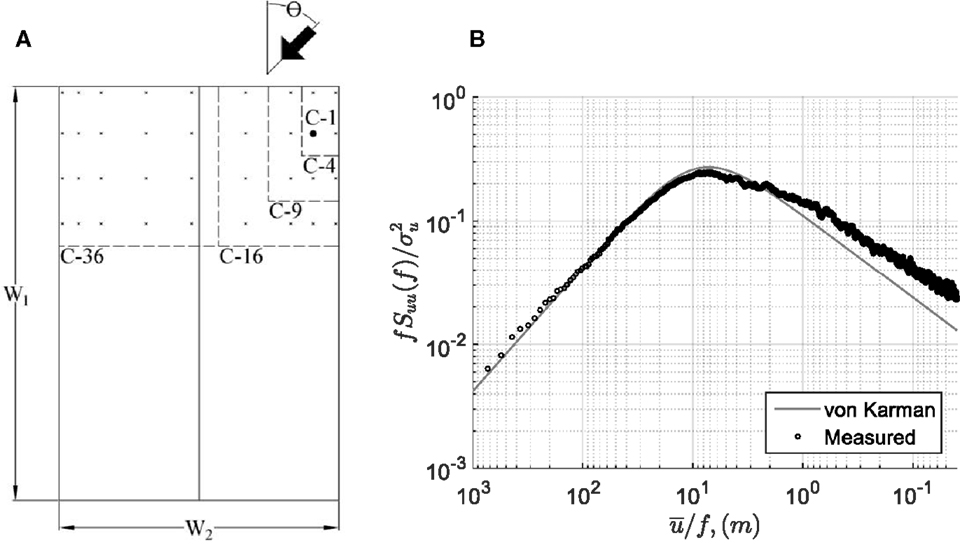
Figure 1. (A) Definition sketch of the 1/50 TTU building model showing the pressure taps used in current analysis and the definition of wind azimuth, θ. (B) Spectra of longitudinal velocity fluctuation at roof height.

A Cobra probe (TFI Corp., Model #289) was place 1H above the leading edge of the roof surface at the mid-plane of the long wall. The location of the cobra probe was selected to obtain the velocities representative of the flow at the building location, while minimizing the effects on the building pressures. We note that several simultaneous cobra probe measurements were made in the experiments. Since the correlation of signals measured between probes decreases significantly as the transverse separation distance increases, the velocity signal measured from the cobra probe above the roof was used as reference for analyses throughout this paper. Furthermore, the cobra probe was fixed to the position with respect to the building for each mean wind azimuth angle in order to analyze the velocity-pressure data using QS theory. The synchronized pressure and velocity time series were sampled at 625 Hz for 200 s for each mean wind direction.

Although there are total 204 pressure taps distributed nearly uniformly on the building model, pressures measured at various corner regions of the roof are selected for analyses in this paper. The selected single tap in the corner region is denoted as case C-1 and shown in Figure 1A. Various portions of roof area-averaged pressures are also shown in Figure 1A. These regions include 4, 9, 16, and 36 pressures taps, which are denoted as C-4, C-9, C-16, and C-36, respectively.

A “suburban” atmospheric turbulent boundary layer wind environment was created by distributing the roughness elements on the tunnel floor between the inlet and the building site. Three 122-cm tall spires and a 38-cm tall barrier were also placed at the inlet of the tunnel. The mean values of the velocity vector measured in this terrain by the cobra probe without the building in place are: $\overline{V}=10.5\text{m/s}$, $\overline{\mathrm{\theta }}\approx \overline{\mathrm{\beta }}\approx 0°$. The probability distributions of the velocity components were found to be nearly Gaussian with the SDs: σ_V = 2.2 m/s, σ_θ = 9.2°, and σ_β = 7°. The integral length scale in the flow direction is nearly 1 m at the roof height. The streamwise velocity spectrum is provided in Figure 1B and shows a reasonable match to the von Karman spectra for the low-frequency portion but has slightly higher energy for the high-frequency region.

Results and Discussions

Quasi-Steady Model

In this section, the QS coefficients are obtained, using the methods described in Section “Quasi-Steady Vector Model.” Because of the symmetric shape of the building and the pressure tap layout, the measurements between $\overline{\mathrm{\theta }}\hspace{0.17em}={\mathrm{\hspace{0.17em}0}}^{°}$ and 90° can be extended to full range of mean wind directions. Figure 2 shows the measured and Fourier-fitted values of E[C_p] for a pressure tap near the roof corner, C-1. By specifying an error threshold for fitting of R² ≥ 99.5%, a total nine orders of Fourier coefficients were used to fit the measured values of E[C_p]. Using the continuous form of E[C_p] from the fit, the instantaneous pressure coefficients, C_p(θ), were solved by the iteration procedure described in Section “Model Construction” and fitted using Eq. 7. The resulting Fourier function representing C_p(θ) is also shown in Figure 2 for case C-1. As found by Richards et al. (1995), differences in magnitudes of C_p(θ) and E[C_p] are observed, particularly for wind directions that cause peak pressures (e.g., for θ near 75° in Figure 2). This is attributed to the averaging process; i.e., the instantaneous azimuth sways about the mean value lead to a smoothing of the E[C_p] curve.

FIGURE 2

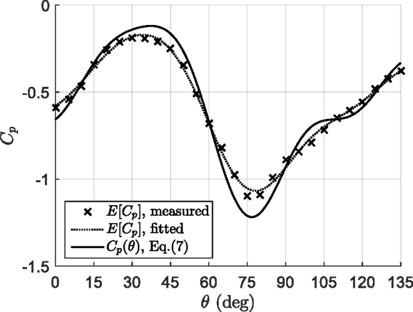
Figure 2. E[C_p] obtained from each mean wind azimuth $\overline{\mathrm{\theta }}$ along with the resulting C_p(θ) described by Eq. 7 for pressure tap, C-1.

Once the instantaneous pressure coefficients are obtained, it is useful to investigate the effects of elevation angle. By using a similar approach as that of Banks and Meroney (2001), the wind-pressure data were first sorted and the data associated with the elemental instantaneous wind azimuth band were identified, i.e., θ − dθ/2 ≤ θ < θ − dθ/2. These data were further separated into three bands associated with the fluctuating elevation angles, i.e., −50° ≤ Δβ < −2.5°, −2.5° ≤ Δβ < 2.5°, and 2.5° ≤ Δβ < 50°, where $\mathrm{\Delta \beta }=\mathrm{\beta }-\overline{\mathrm{\beta }}$. These three ranges were chosen for plotting and represent downward-acting, nearly horizontal, and upward-acting wind angles, respectively. The measured C_p(θ, β) were obtained by averaging for the condition of these three elevation-angle bands, as indicated by Eq. 5. The conditional averaging was repeated for the elemental azimuth band for several mean wind directions. Figure 3 shows the resulting measured values of C_p(θ, β) in discrete symbols along with the fit-C_p(θ) curve (described by Eq. 7) for pressure tap C-1 for four mean azimuths. Because the total number of data points used for each C_p(θ, β) value are different, the attached gray-scale denotes the equivalent duration used in conditional averaging the data (i.e., number of data points divided by sampling rate), since there are relatively few data points for large excursions from the mean.

FIGURE 3

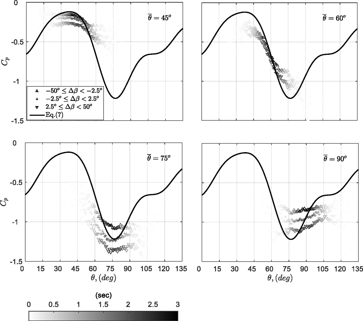
Figure 3. E[C_p,inst|θ, β] and C_p(θ) (represented by Eq. 7) for case C-1, mean wind azimuths $\overline{\mathrm{\theta }}$ = 45°, 60°, 75°, and 90°.

As can be seen in Figure 3, both the magnitude of the coefficients and the functional variations with θ are dependent on the elevation angle for pressure tap C-1. Regarding the functional variations, the C_p(θ, β) variations are found to follow the fit-C_p(θ) curve from Figure 2 for θ ≤ 75°, while keeping the same trend but with much milder slopes for θ > 75°. Banks and Meroney (2001) first reported similar effects. These authors attributed it to a hysteresis effect such that the instantaneous pressures could not respond to the fluctuations in the wind direction. For example, conical (or corner) vortices dominate the flow structure and the corresponding low pressures at the tap C-1 for mean wind azimuth $\overline{\mathrm{\theta }}\hspace{0.17em}={\mathrm{\hspace{0.17em}75}}^{°}$. When the instantaneous wind suddenly sways to $\mathrm{\theta }\hspace{0.17em}={\mathrm{\hspace{0.17em}90}}^{°}$, this flow structure does not change to separation bubble type of flow found observed at $\overline{\mathrm{\theta }}\hspace{0.17em}={\mathrm{\hspace{0.17em}90}}^{°}$ and, therefore, retrieve the instantaneous pressure. The reverse situation is true for $\overline{\mathrm{\theta }}\hspace{0.17em}={\mathrm{\hspace{0.17em}90}}^{°}$, as shown in Figure 3.

The fluctuating wind elevations also play a role in affecting the magnitude of the pressures at tap, C-1. In general, an upward wind (i.e., Δβ > 0) leads to higher suctions, while a downward wind (i.e., Δβ < 0) leads to lower suctions, with the degree of influence depending on the wind azimuth. Similar observations were also presented by Letchford and Marwood (1997) Sharma and Richards (1999) and Richards and Hoxey (2004). As expected, the measured values of C_p(θ, β) tend to be closest to the fit-C_p(θ) curve (from Figure 2) for horizontal winds (i.e., Δβ ≈ 0), at least for $\mathrm{\theta }\hspace{0.17em}=\overline{\mathrm{\theta }}$. In order to further investigate the elevation-angle effects on the magnitude of C_p(θ, β), we examine the measured differences of the coefficients, $C_{\text{p}}\left(\mathrm{\theta },\mathrm{\beta }\right)-C_{\text{p}}\left(\mathrm{\theta },\overline{\mathrm{\beta }}\right)$. Figure 4 shows the results, which were obtained for a 5°-band of wind azimuth around the mean (i.e., −2.5° ≤ Δθ < 2.5°, where $\mathrm{\Delta \theta }=\mathrm{\theta }-\overline{\mathrm{\theta }}$). As in Figure 3, the gray-scale in the figure denotes the total number of data points used in conditional averaging as an effective duration. Because the changes caused by the elevation angles to the instantaneous pressure coefficients are found to be linear (in most cases), a linear fit with zero intercept at Δβ = 0 is also plotted in the figure. This fitting procedure was conducted for each mean wind azimuth and the corresponding gradients, B = dC_p/dβ, were calculated. Figure 5 depicts the resulting gradients for each mean azimuth, along with a Fourier-series fit described by Eq. 9.

FIGURE 4

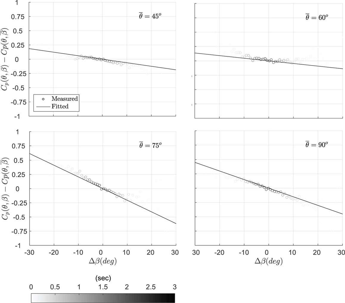
Figure 4. The variation of C_p versus Δβ obtained from data points within azimuth band −2.5° ≤ Δθ < 2.5° for case C-1, mean azimuths $\overline{\mathrm{\theta }}$ = 45°, 60°, 75°, and 90°.

FIGURE 5

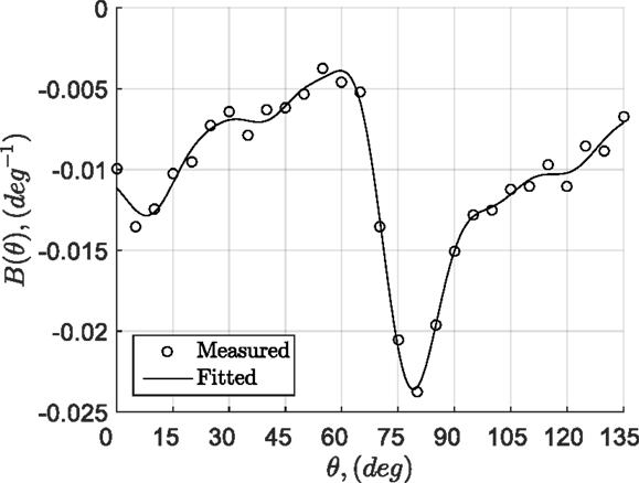
Figure 5. The B(θ) obtained from data points within azimuth band −2.5° ≤ Δθ < 2.5° for each mean wind azimuths for case C-1.

Since there are clear variations of C_p(θ, β) for different ranges of wind elevation angle, it is worthwhile to look at the corresponding conditionally averaged elevation angles, E[Δβ|θ], for each elemental azimuth band θ ≡ {Δθ − dθ/2 ≤ Δθ < Δθ − dθ/2} for wind vector time series obtained without the building in place. Figure 6A shows the joint pdf for the fluctuating azimuth and fluctuating elevation angle, f(Δθ, Δβ). The nearly concentric shape of probability distribution data indicates a low correlation between Δθ and Δβ. Therefore, the E[Δβ|θ] locus is quite uniform and nearly equal to +7°, 0°, and −7° for the upward, horizontal, and downward bins of elevation angle, respectively, as shown in Figure 6B. Although upward-acting winds increase |C_p| at pressure tap C-1, as shown by Figures 3 and 4, the existence of Reynolds stresses, $-\overline{uw}$, in the atmosphere boundary layer has been reported by Sharma and Richards (1999) to suppress such fluctuations. Basically, the Reynolds shear stresses imply that the positive gusts (i.e., increasing horizontal wind speeds) are generally associated with negative elevation angles. This can be observed by Figure 6C, where the joint pdf between velocity-square ratio, $V^2\left(\mathrm{\Delta \beta }\right)/V^2\left(\overline{\mathrm{\beta }}\right)$, and fluctuating elevation angle, Δβ, were obtained with the building removed from the wind tunnel. A clear negative correlation between $V^2\left(\mathrm{\beta }\right)/V^2\left(\overline{\mathrm{\beta }}\right)$ and Δβ can be observed. Thus, based on Eq. 10, instantaneously high values of dynamic pressure are generally offset by instantaneous pressure coefficients of lower magnitude, leading to the suppression process of the surface pressures. For events such as tornadoes, however, Reynolds stresses effects, and, in fact, the role of the vertical component of the wind, in general, is a largely unexplored issue. Thus, upward wind directions produced by these types of storms may induce roof pressures beyond the expectations obtained from typical boundary layer wind experiments.

FIGURE 6

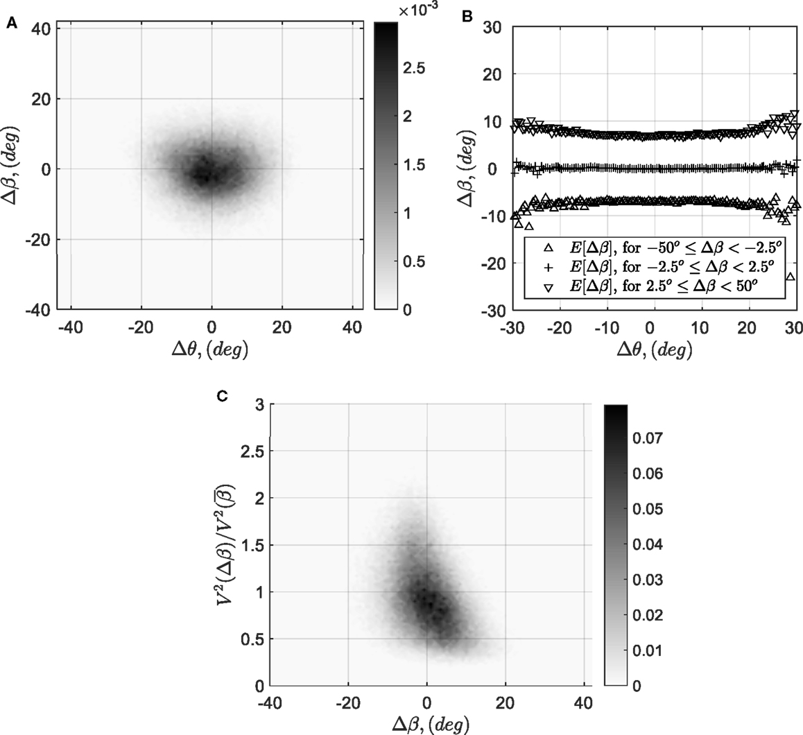
Figure 6. (A) f(Δθ, Δβ), (B) E[β] loci for given ranges of β, and (C) $f\left(\mathrm{\Delta \beta },V^2\left(\mathrm{\Delta \beta }\right)/V^2\left(\overline{\mathrm{\beta }}\right)\right)$ obtained from velocity measurement without building in place.

Comparison of Measured and Quasi-Steady Theory Predicted Pressures

In this section, the QS model described in Eq. 10 is used to calculate the typical pressure coefficients, C_p,t (defined in Eq. 1), and compared to measurements. Two forms of the model are used: one that only accounts for the instantaneous wind azimuth contribution (QS-θ), which utilizes only the $C_{\text{p}}\left(\mathrm{\theta },\overline{\mathrm{\beta }}\right)$ term in Eq. 8, and the other that includes both azimuth and elevation angles (QS-θ-β), i.e., the full model defined in Eq. 8. The analysis involves four cases, including single point pressures (C-1) and area-averaged pressures (C-4, C-9, and C-16, as defined in Figure 1).

Figure 7 shows the spectra of measured and QS estimates of C_p,t for the four areas and the mean wind azimuth of 75°. Generally, both the distribution and magnitude of the spectra obtained from QS models are similar to measurements. In general, the spectra obtained via the QS-θ model are found to be slightly higher in magnitude than the QS-θ-β prediction, which can be explained by the suppression process of pressure fluctuation when the wind elevation is included, as discussed by Sharma and Richards (1999) and in Section “Quasi-Steady Model.” The QS-θ-β model generally gives spectra of slightly lower magnitude compared to the measurements.

FIGURE 7

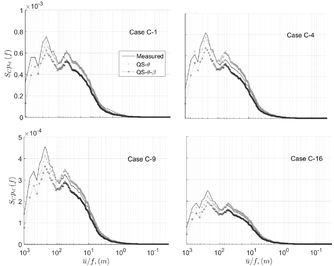
Figure 7. Spectra of measured and quasi-steady predicted C_p,t for cases C-1, C-4, C-9, and C-16, mean wind azimuth $\overline{\mathrm{\theta }}$ = 75°.

The frequency-dependent correlation coefficient between the measured and QS-predicted values of C_p,t is also of interest. For this purpose, the real part of the coherence obtained from the normalized cross-spectra between measured and QS-predicted C_p,t values,

$\mathrm{\eta }\left(f\right)=\frac{\mathrm{Re}\left[S_{\text{QS},\text{m}}\left(f\right)\right]}{\sqrt{S_{\text{QS}}\left(f\right)}\sqrt{S_{\text{m}}\left(f\right)}}$ (19)

is calculated, where S_QS(f) and S_m(f) denote the auto-spectra of QS-predicted and measured C_p,t at frequency, f, respectively, and S_QS,m(f) is the cross-spectra between the prediction and the measurement. Figure 8 shows the calculated values of η for the four areas and a mean wind direction of 75°. Generally, the QS-predicted C_p,t fluctuations are a better match for larger gusts, with η ≈ 0.9 for ū/f ≥10 m, noting that the integral scale is about 1 m and the largest building length is 0.275 m. The level of correlation begins to decrease for $ū/f<10\text{(m)}$ and is ≈ 0 for $ū/f<1\text{(m)}$. Although low η are found for small gust sizes, the C_p,t fluctuations are relatively low over this region, as can be seen in the auto-spectra plots (Figure 7). Furthermore, the QS-θ-β predictions are seen to have better correlations with the measured values, especially in middle range of frequencies ($0.5\left(\text{m}\right)<ū/f<10\text{(m)}$), when compared to the QS-θ estimates.

FIGURE 8

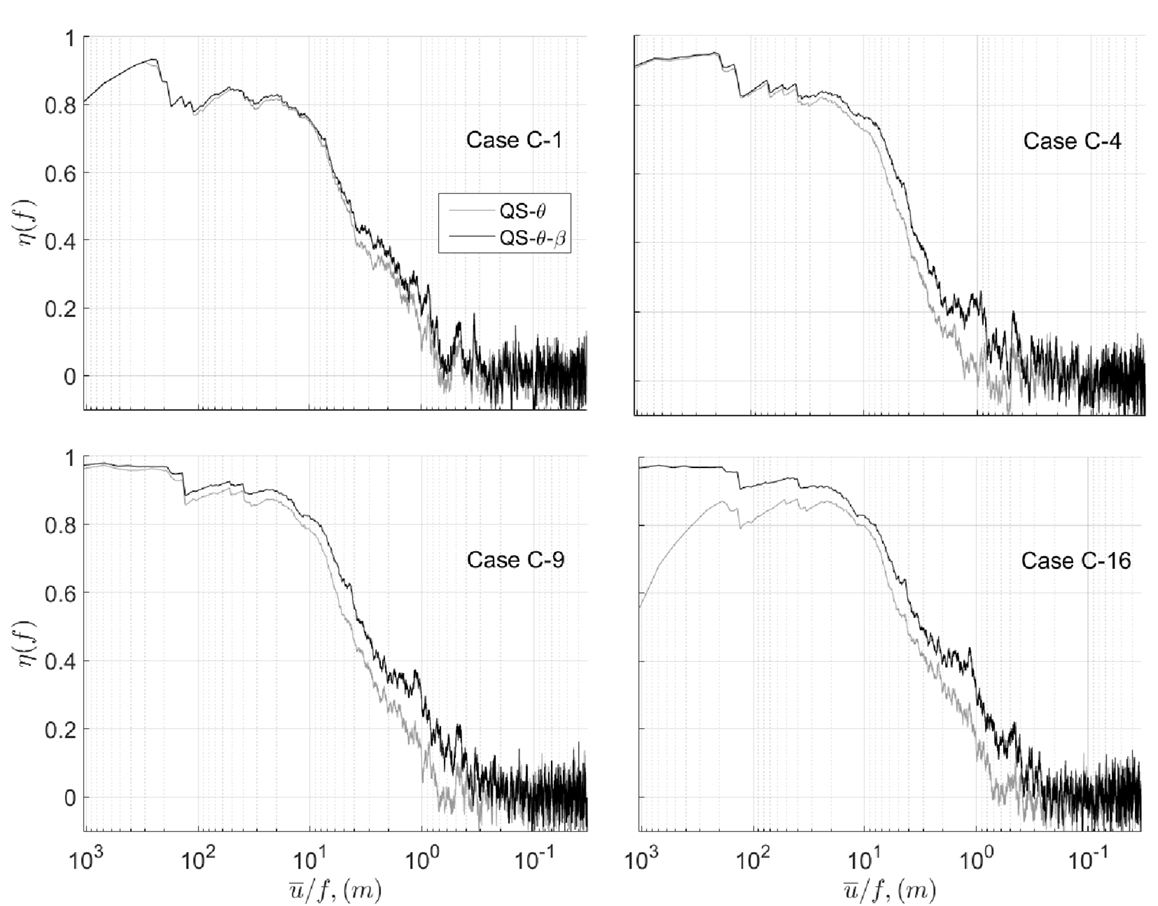
Figure 8. Coherence between measured and QS-predicted C_p,t for cases C-1, C-4, C-9, and C-16, mean wind azimuth $\overline{\mathrm{\theta }}$ = 75°.

To better understand the impact of the results depicted in Figures 7 and 8; Figure 9 shows the measured and (QS-θ-β)-predicted time series for 3 s around a selected peak denoted as time, t = t_p. The figure indicates that the low-frequency portion of the fluctuations follow the measurements for case C-1, while the tracking of the time series at higher frequencies is clearly lacking, leading to underestimations of predictions near peak values, with differences up to 30% are observed. The better correlation of low-frequency portion is a reflection of case C-1 of Figure 8, while the underestimation of peaks may be attributed to underestimation of the spectral content for both the low and median frequency ranges of Figure 7. When more points were included in area-averaging, a gradual improvement in the QS-θ-β predictions can be observed for cases C-4, C-9, and C-16 in Figure 9. This may be because of the fact that the area-averaging of closely spaced point pressures acts like a low-pass filter of the individual point pressures, which removes the low-correlation/high-frequency portion of C_p,t predicted by the model. This observation of low-pass spatial filtering process was first discussed by Letchford et al. (1993) from their analysis of full-scale measurements (noting that a linear QS-θ model was used in their work).

FIGURE 9

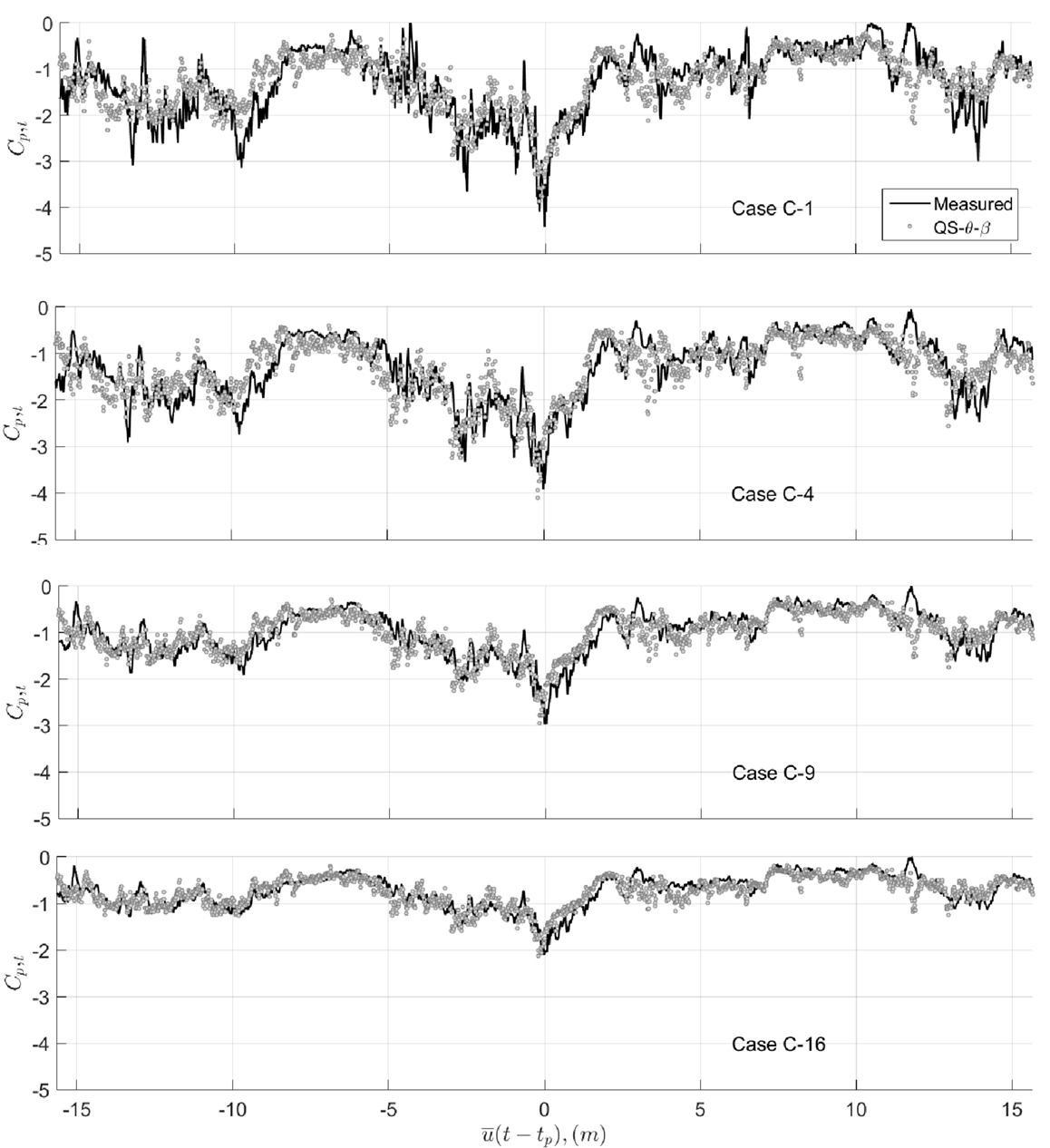
Figure 9. Time series of measured and QS-predicted C_p,t around a selected peak for cases C-1, C-4, C-9, and C-16, mean wind azimuth $\overline{\mathrm{\theta }}$ = 75°.

Finally, the zero-time-lag correlation coefficients between the measured and predicted coefficients are shown in Figure 10, for the four areas and all mean wind azimuths. For pressure tap C-1, the correlation coefficients were found to be nearly uniform with wind direction and approximately equal to 50%, except for mean wind azimuths ${10}^{°}<\overline{\mathrm{\theta }}<{55}^{°}$. For area-averaged cases, the correlation coefficients are nearly uniform across all of the measured mean wind azimuths and gradually increases as the number of pressure taps included in the average increase, reaching 65% for the QS-θ-β model over the interval, ${40}^{°}\le \overline{\mathrm{\theta }}\le {90}^{°}$. Such improvements, again, can be explained by the low-pass filtering induced by the area-averaging process and indicate that the QS models are more appropriate for area-averaged pressures (see also Letchford et al., 1993). The differences between the QS-θ and QS-θ-β models can also be observed in terms of correlation coefficients in Figure 10. Generally, the QS-θ-β model gives better-correlated predictions than QS-θ-β model, with the magnitudes of the differences depending on wind azimuth. The differences become more uniform for area-averages. Because of the better performance of the QS-θ-β model, it is selected for analyses for the following sections.

FIGURE 10

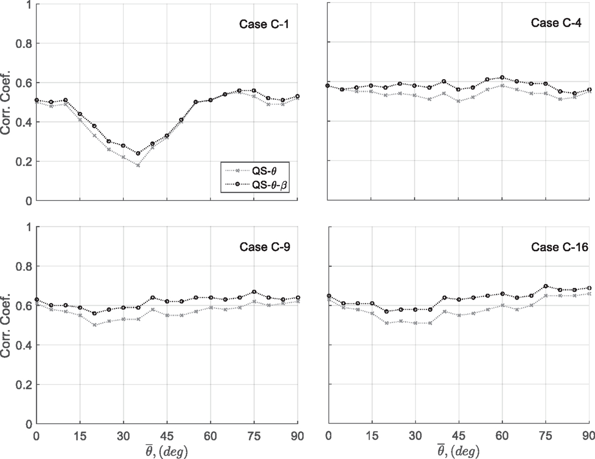
Figure 10. Zero-time-lag correlation coefficient between measured and QS-predicted C_p,t for cases C-1, C-4, C-9, and C-16.

Statistics of Measured and Estimated Pressures

In this section, the statistics of C_p,t time histories obtained from measurements and the QS-θ-β model are compared. Figure 11A shows the pdf of the measured and predicted values for case C-1 with a mean wind direction of 75°. Of note, the statistical method based on QS theory, described in Section “Use of QS Model to Calculate Pressure Statistics,” was used to obtain the pdf and is denoted as “QS-statistics.” These results are compared to those obtained directly from the estimated time history (using wind vector with the QS assumption), labeled as “QS-TH.” The nearly equivalent values of the QS-TH and QS-statistics validate the use of the statistical method. Thus, the results using the method in Section “Use of QS Model to Calculate Pressure Statistics” (QS-statistics) are presented in what follows, eliminating the need for calculating the time histories.

FIGURE 11

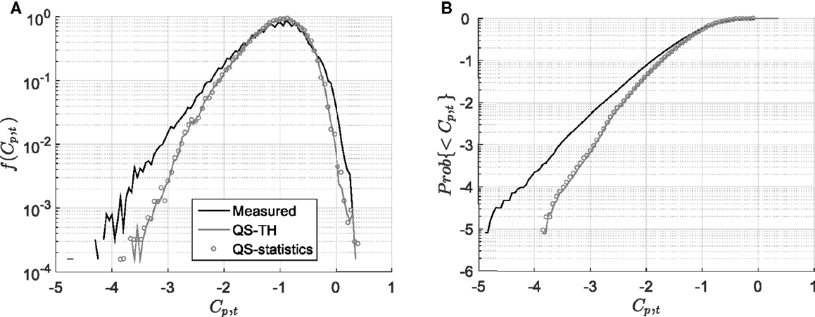
Figure 11. (A) Pdf and (B) cdf of C_p,t’s obtained from measurement and QS-θ-β model for case C-1 for mean wind azimuth $\overline{\mathrm{\theta }}$ = 75°.

Figure 11 indicates that the QS-θ-β model underestimates the peak values at tails of the distribution, consistent with the observations from the C_p,t time-series segments shown in Figure 9. Figure 11B further shows that the corresponding cumulative density functions (cdf), Prob{<C_p,t}, which is the probability of a typical pressure coefficient below a given value, is able to predict the probability of exceedance up to 0.3 but underestimates the values for probabilities of exceedance below 0.3. If a probability of exceedance of 0.01% is selected as the reference, the corresponding estimated peak value, C_p,t = −3.5, is 17% lower than the measured peak, C_p,t = −4.2.

Although the statistical method derived in Section “Use of QS Model to Calculate Pressure Statistics” is for point pressures, it can easily be extended to area-averaged pressures. This is done by simply replacing $C_p\left(\mathrm{\theta },\overline{\mathrm{\beta }}\right)$ and B(θ) with the appropriate area-averaged values, $w_{\text{i}}{C}_{\text{p,i}}\left(\mathrm{\theta },\overline{\mathrm{\beta }}\right)$ and w_iB_i(θ), respectively, in Eq. 8, where w_i denotes the weight for pressure tap, i. Figure 12 depicts the cdfs of four area-averaged coefficients obtained from measurements and prediction for a mean wind direction of 75°. Again, if 0.01% is selected as the reference probability of exceedance, the (QS-θ-β)-predicted peak C_p,t = −3.5 is now 13% less than the measured peak C_p,t = −4.0 for C-4. Thus, the underestimation is reduced compared to the C-1 case. The estimates continue to be improved as the total number of taps included in the area increases, and eventually, the (QS-θ-β)-predicted distributions are found to closely match the measurement cases, here for C-16 and C-36. The improvement of the QS-θ-β statistical method for area-averaged pressures is consistent with the observations found in QS-θ model by Letchford et al. (1993).

FIGURE 12

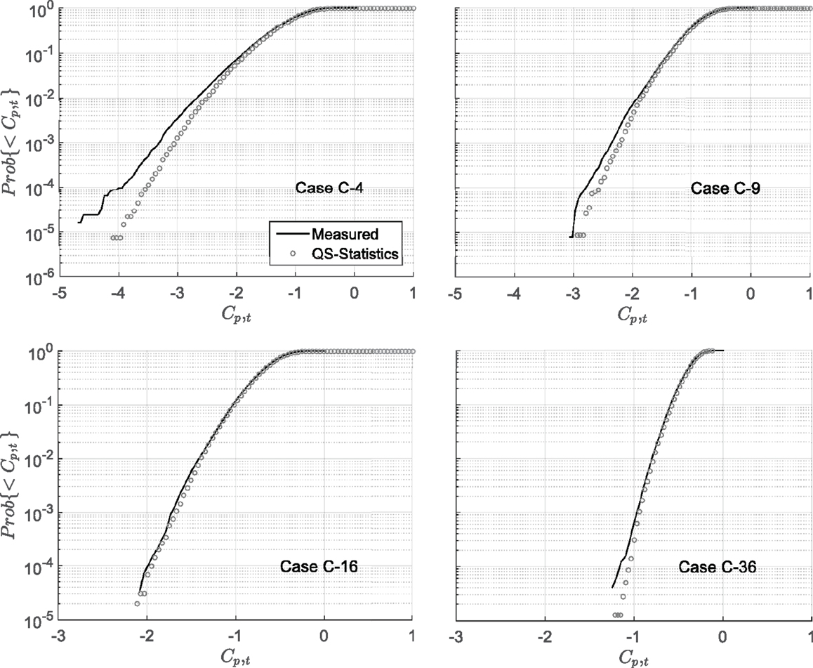
Figure 12. Cdf of C_p,t’s obtained from measurement and QS-θ-β model for cases C-4, C-9, C-16, and C-36, mean wind azimuth $\overline{\mathrm{\theta }}$ = 75°.

To further investigate the general capability of the QS-θ-β statistical method, the peak pressure coefficients based on the 0.01% probability of exceedance were calculated and compared with measurements in Figure 13 for the four area-averages, for all measured mean wind azimuths. For case C-4, although the peaks predicted by QS follow the trend observed in measurement, the QS-predicted peaks underestimated the observed values for all wind directions, with larger values for the cases where $\overline{\mathrm{\theta }}\le {25}^{°}$ and $\overline{\mathrm{\theta }}\ge {75}^{°}$. As for the results presented in Figure 12, the overall level of underestimation of QS-predicted peaks was reduced when more taps are included in the area-averages. Excellent results are obtained for case C-36, although C-16 also is very good.

FIGURE 13

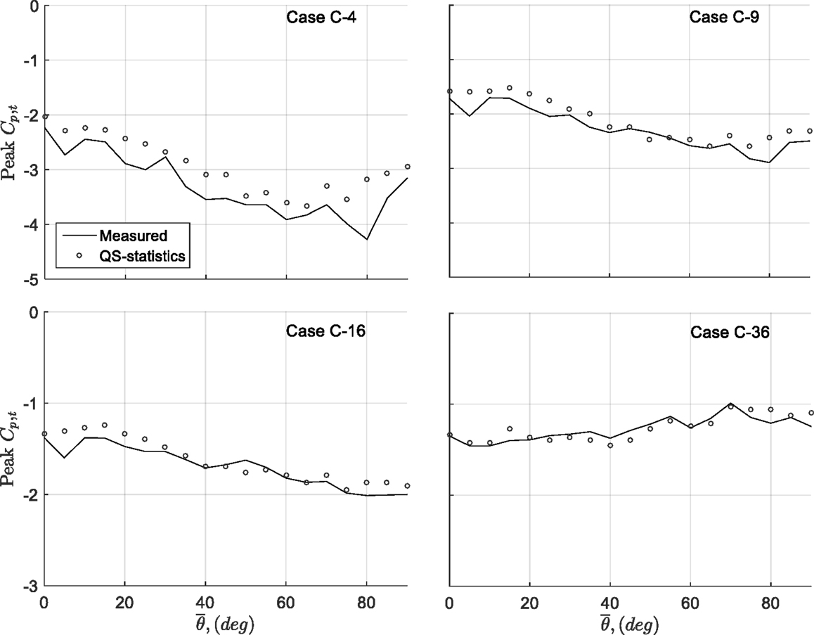
Figure 13. Peak C_p,t’s obtained from measurement and QS-θ-β model for cases C-4, C-9, C-16, and C-36.

Finally, some comments are made about the statistical model described in Section “Use of QS Model to Calculate Pressure Statistics,” given by Eqs. 17 and 18, and the data used herein. First, the joint pdf of the wind vector, $f\left(V/\overline{V},\mathrm{\theta },\mathrm{\Delta \beta }\right)$, was found not to be reduced to the individual multiplication, $f\left(V/\overline{V}\right)f\left(\mathrm{\theta }\right)f\left(\mathrm{\Delta \beta }\right)$, because of a lack of mutual independence between the instantaneous velocity ratio, wind azimuth, and elevation angle. Therefore, our use of $f\left(V/\overline{V},\mathrm{\theta },\mathrm{\Delta \beta }\right)$ is different from the use of $f\left(V/\overline{V}\right)f\left(\mathrm{\theta }\right)f\left(\mathrm{\Delta \beta }\right)$ in Richards and Hoxey (2004). However, the velocity ratio and wind azimuth have been found to be independent so that the individual multiplication, $f\left(V/\overline{V}\right)f\left(\mathrm{\theta }\right)$, can replace the joint pdf, $f\left(V/\overline{V},\mathrm{\theta }\right)$ when the QS-θ model is applied (e.g., Banks and Meroney, 2001; Richards and Hoxey, 2004).

Second, the joint pdf, $f\left(V/\overline{V},\mathrm{\theta },\mathrm{\Delta \beta }\right)$, used in this paper was obtained from a fixed position with respect to the building for each mean wind azimuth, which leads to questions about the possible distortion of measurements due to the building. Measurements showed that there is little difference between the joint pdf of the fluctuating quantities (i.e., $f\left(V/\overline{V},\mathrm{\Delta \theta },\mathrm{\Delta \beta }\right)$) measured with and without the building in place, with R² values around 95% for all mean wind azimuths. Although there are indeed some small changes of the mean quantities (i.e., $\overline{V},\overline{\mathrm{\theta }},\text{\hspace{0.17em}and\hspace{0.17em}}\overline{\mathrm{\beta }}$) due to the placement of the building, there is no influence on evaluating the probability distributions based on the formulation described in Eq. 17. However, small changes in mean wind speed may be considered in Eq. 18 for evaluating the probability distributions of surface pressures.

Third, because the current building can be viewed as a sharp-edged bluff body, the typical pressure coefficients measured on the roof are largely Reynolds number independent (Holmes, 2001). Thus, the statistical model in Eqs. 17 and 18 is a convenient tool for predicting the probability distributions of roof surface pressure over a range of mean wind speeds, presuming there are no changes in the structure of the wind with wind speed. These invariant joint pdfs of the wind speed vector can be coupled with the instantaneous pressure coefficients, leading to an invariant distribution of C_p,t, based on Eq. 17. Therefore, the pdf of roof surface pressures can be obtained by simply changing the mean wind speed, $\overline{V}$, in Eq. 18. Once the pdf of surface pressured is obtained, other statistical quantities, e.g., probability of exceedance, can be derived. For example, Figure 14 shows the probability of the building surface pressure exceeding −2 kPa for mean wind speeds ranging from 30 to 170 m/s for the four area-averages (C-4, C-9, C-16, and C-36) for a 75° mean wind azimuth. These curves mimic “fragility” curves, but are simplified examples with the assumption of a fixed holding strength. Actual fragility curves can be obtained by including the statistics of the panel holding strengths and more accurate failure mechanism; however, the QS statistical model of Eq. 17 or 18 can be used to simplify the process of accurately modeling the variations of the wind load.

FIGURE 14

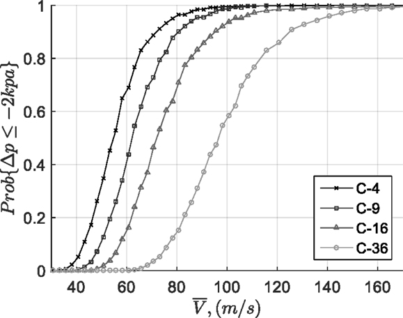
Figure 14. Probability of QS-θ-β predicted pressures below −2 kpa for cases C-4, C-9, C-16, and C-36 for mean wind azimuth $\overline{\mathrm{\theta }}$ = 75°.

Discussion on General Applicability and Future Work

In this section, the general applicability of QS-θ-β model is addressed, based on the results obtained here and in earlier publications, along with some expectations and future work based on these findings. For components of the roof that have small areas typical of Components and Cladding loads (e.g., areas represented by C-1 and C-4 in Figure 1A), a non-negligible portion of the fluctuation energy is missing and the QS-θ-β model is only able to account for a portion of the pressure fluctuations (Figures 9 and 11). This missing fluctuation energy, with resulting under-estimated peak values, is largely due to building generated turbulence and other unsteady effects. For example, the hysteresis effects identified by Banks and Meroney (2001) are an example where winds shift direction such that the vortex structure on the roof is altered but not in a way that the instantaneous pressures match the mean flow patterns at the actual wind direction. For winds that are perpendicular to the roof edge, the largest suctions acting near the roof edge are produced by transient vortices created near the edge at a point in time when the mean separation bubble is largely non-existent (Pratt and Kopp, 2014) following processes first described by Saathoff and Melbourne (1997). Such situations create difficulty for QS theory when applied to small areas. The threshold for defining “small” scale is ~10H (or, around 1 m for the model in the current study), or gusts that fully envelope the entire building, as suggested by the coherence plots in Figure 8 and discussed in Section “Comparison of Measured and Quasi-Steady Theory Predicted Pressures.” Evidently, these effects are localized since the QS method is able to capture the full range of fluctuations when averaged over larger areas, at least for flat roofs, as in the current study (as well as in Letchford et al., 1993). However, based on this, it is not clear how applicable QS estimation of larger-area pressures would be for scenarios when there are more complex roof shapes such as hip roofs, which have local separation points at multiple edges (e.g., Gavanski et al., 2013). Thus, the applicability of QS method for such buildings is necessary in a future study.

In terms of other practical applications, the QS method is anticipated to provide a useful tool for pressure estimation during transient storms (e.g., microbursts, downbursts, tornadoes, etc.). Due to the rapid spatial translation of these types of wind storms, buildings in their path can experience rapid and intense changes of wind speed and direction, especially when compared to the movements and development of large-scale synoptic storms. These storms produce different wind fields that can have features such as upwardly directed gusts correlated with high wind speeds, different vortex structures, and other particular features. Of particular interest is the vertical component of the wind. For example, Blanchard (2013) found that the elevation angle could be more than 20° at the moment when a tornado has its most intense horizontal wind speeds. This contrasts with typical atmospheric surface layers, where gust speeds are generally correlated with downward-acting winds (as noted earlier in Section “Statistics of Measured and Estimated Pressures” and Figure 6C). Because the upward wind is generally associated with higher pressure coefficients on roofs (as shown in Figures 3–5), building surface pressures may be amplified in the tornado-induced wind, as compared to typical boundary layer winds, given similar dynamic pressures and that the QS model holds for both scenarios. Further work is required to identify whether the linear relationship between pressure and elevation angle holds, or whether a non-linear contribution may be required in order to maintain accurate estimates of C_p(θ, β).

Conclusion

The QS model assumes the instantaneous surface pressure as a multiplication of instantaneous dynamic pressure, 0.5ρV², with the instantaneous pressure coefficient, C_p. This method is applied and extended in this paper to relate the wind speed to building surface pressure. The effects of wind azimuth and elevation angle are reflected in the instantaneous pressure coefficient, i.e., C_p(θ, β), in the QS vector model (QS-θ-β) with a linear effect of wind elevation found to be adequate for the range of fluctuating elevation angle, Δβ, such that C_p(θ, β) = C_p(θ) + (dC_p/dβ)Δβ. The gradient dC_p/dβ is found to vary with respect to wind azimuth so that the functional form is fit with a Fourier series. The coefficients in the model were evaluated from synchronized measurements of building surface pressures and local wind speed vectors. The experimental method used here eliminates the need to tilt the building model, which was required in the procedures suggested by the previous work, thereby facilitating a process for establishing the QS-θ-β model. The main conclusions are as follows.

Upward-acting winds (i.e., Δβ > 0) are generally associated with higher magnitudes of C_p while the downward-acting winds (i.e., Δβ < 0) are generally associated with lower magnitudes. The effect of the elevation angle can be as large as the effect of wind azimuths for certain mean incident wind angles. Higher dynamic pressures, however, are generally associated with downward wind in the atmospheric boundary layer leading to a suppression process of the actual observed peaks because of this. These observations are consistent with previous published works. By contrast, tornadoes, which can have significant upwardly directed winds, could have significantly increased wind loads as a result of this.

A statistical method that uses the QS-θ-β model was also derived and validated. With this method, the pdf of building surface pressures is formulated as a double integral of the joint pdf between instantaneous wind speed ratio, wind azimuth, and elevation angle, $f\left(V/\overline{V},\mathrm{\theta },\mathrm{\beta }\right)$. Because no mutual independence is found between V/$\overline{V}$, θ, and β, the joint pdf used here is not further reduced to $f\left(V/\overline{V}\right)f\left(\mathrm{\theta }\right)f\left(\mathrm{\beta }\right)$, a formulation that has been used in previous works. Furthermore, the direct use of joint pdf of wind speed (turbulence) in our formulation offers a more straightforward approach when compared to the procedures used in previous works. Peak pressures were predicted by applying this method and compared to the measured values for all mean incident wind angles. Underestimation of peak pressures was observed for point pressures on the roof. The accuracy of peak prediction increases as the number of points included in area-averages increases. More specifically, the mean level of error (underestimation) was found be about 30% for a single pressure tap, while this reduces to <5% for area-averages of 16 and 36 taps (on the current building with the current tap layout). Thus, the proposed QS-θ-β model is found to perform well for roof pressure estimation when relatively large areas of the roof are considered for this typical low-rise building. Future work will focus on the applicability of the proposed method to roofs with more complex geometries. One potential use of the statistical method derived here may be in calculating fragility curves for storms with different durations.

Author Contributions

C-HW is a Ph.D. student under the supervision of GK and this research is a portion of what will become C-HW’s doctoral thesis. The experiments and approach were designed collaboratively by the authors. The manuscript was written collaboratively; C-HW wrote the first draft. The experiments, the direct analysis of the experimental data, and the development of the quasi-steady model equations were conducted by C-HW, with direct input from GK.

Conflict of Interest Statement

The authors declare that the research was conducted in the absence of any commercial or financial relationships that could be construed as a potential conflict of interest.

Funding

This work was funded by NSERC through the Collaborative Research and Development (CRD) program.

Nomenclature

B	The gradient dCp/dβ.
Cp	Estimated instantaneous pressure coefficient, E[Cp,inst].
Cp,inst	Instantaneous pressure coefficient, p − p0/(0.5ρV2).
Cp,t	Typical pressure coefficient, $p-p_0/\left(0.\mathrm{5\rho }{\overline{V}}^2\right)$.
J	Jocobian determinant.
N1, N2	Total orders used in Fourier series.
Sa	Spectra of the quantity a.
Sa,b	Cross-spectra between quantities a and b.
V	Total velocity.
a1, b1	Fourier coefficients for functions Cp(θ).
a2, b2	Fourier coefficients for functions B(θ).
f	Frequency.
k	Integer counter.
p	Pressure.
p0	Ambient static pressure.
Δp	Pressure difference, p − p0.
tp	The time corresponding to peak Cp,t.
u	Longitudinal velocity component.
v	Transverse velocity component.
w	Vertical velocity component.
wi	Weight of i-th tap used in area averaging.
y1, y2	Auxiliary variables.
β	Wind elevation.
Δβ	Wind elevation fluctuation, $\mathrm{\beta }-\overline{\mathrm{\beta }}$.
ε	Residual used in iteration process.
η	Real part of coherence function.
θ	Wind azimuth.
Δθ	Wind azimuth fluctuation, $\mathrm{\theta }-\overline{\mathrm{\theta }}$.
ρ	Air density.
σa	Standard deviation of the quantity a.
{a}	Event a.
$E\left[a\right],ā$	Mean (or estimate) of a.
E[a|b]	Mean (or estimate) of a based on the condition b.
f (a)	Probability density function (pdf) of a.
(a)r	Root value of a.
Re[a]	Real part of a.

References

Banks, D., and Meroney, R. N. (2001). The applicability of quasi-steady theory to pressure statistics beneath roof-top vortices. J. Wind Eng. Ind. Aerodyn. 89, 569–598. doi: 10.1016/S0167-6105(00)00092-1

CrossRef Full Text | Google Scholar

Blanchard, D. O. (2013). A comparison of wind speed and forest damage associated with tornadoes in northern Arizona. Weather Forecast. 28, 408–417. doi:10.1175/WAF-D-12-00046.1

CrossRef Full Text | Google Scholar

Cook, N. J. (1990). The Designer’s Guide to Wind Loading of Building Structures, Part 2 Static Structures. UK: Butterworths.

Google Scholar

Gavanski, E., Kordi, B., Kopp, G. A., and Vickery, P. J. (2013). Wind loads on roof sheathing of houses. J. Wind. Ind. Aerodyn. 114, 106–121. doi:10.1016/j.jweia.2012.12.011

CrossRef Full Text | Google Scholar

Ho, T. C. E., Surry, D., Morrish, D., and Kopp, G. A. (2005). The UWO contribution to the NIST aerodynamic database for wind loads on low buildings: part 1. Archiving format and basic aerodynamic data. J. Wind Eng. Ind. Aerodyn. 93, 1–30. doi:10.1016/j.jweia.2004.07.006

CrossRef Full Text | Google Scholar

Holmes, J. D. (2001). Wind Loading of Structures. London: Spon Press.

Google Scholar

Kawai, H. (1983). Pressure fluctuations on square prisms – applicability of strip and quasi-steady theories. J. Wind Eng. Ind. Aerodyn. 13, 197–208. doi:10.1016/0167-6105(83)90141-1

CrossRef Full Text | Google Scholar

Letchford, C. W., Iverson, R. E., and McDonald, J. R. (1993). The application of the quasi-steady theory to full scale measurements on the Texas Tech Building. J. Wind Eng. Ind. Aerodyn. 48, 111–132. doi:10.1016/0167-6105(93)90284-U

CrossRef Full Text | Google Scholar

Letchford, C. W., and Marwood, R. (1997). On the influence of v and w component turbulence on roof pressures beneath conical vortices. J. Wind Eng. Ind. Aerodyn 69-71, 567–577.

Google Scholar

Papoulis, A., and Pillai, S. U. (2002). Probability, Random Variables and Stochastic Processes, 4th Edn. New Delhi: McGraw Hill Inc.

Google Scholar

Pratt, R. N., and Kopp, G. A. (2014). Velocity field measurements above the roof of a low-rise building during peak suctions. J. Wind Eng. Ind. Aerodyn. 133, 234–241. doi:10.1016/j.jweia.2014.06.009

CrossRef Full Text | Google Scholar

Richards, P. J., and Hoxey, R. P. (2004). Quasi-steady theory and point pressures on a cubic building. J. Wind Eng. Ind. Aerodyn. 92, 1173–1190. doi:10.1016/j.jweia.2004.07.003

CrossRef Full Text | Google Scholar

Richards, P. J., and Hoxey, R. P. (2012). Pressures on a cubic building – part 2: quasi-steady and other processes. J. Wind Eng. Ind. Aerodyn. 102, 87–96. doi:10.1016/j.jweia.2011.11.004

CrossRef Full Text | Google Scholar

Richards, P. J., Hoxey, R. P., and Wanigaratne, B. S. (1995). The effect of directional variation on the observed mean and rms pressure coefficients. J. Wind Eng. Ind. Aerodyn. 5, 359–367. doi:10.1016/0167-6105(94)00067-N

CrossRef Full Text | Google Scholar

Saathoff, P. J., and Melbourne, W. H. (1997). Effects of free-stream turbulence on surface pressure fluctuations in a separation bubble. J. Fluid Mech. 337, 1–24. doi:10.1017/S0022112096004594

CrossRef Full Text | Google Scholar

Sharma, R. N., and Richards, P. J. (1999). The influence of Reynold stresses on roof pressure fluctuations. J. Wind Eng. Ind. Aerodyn. 83, 147–157. doi:10.1016/S0167-6105(99)00068-9

CrossRef Full Text | Google Scholar