An Autonomous Strain-Based Structural Monitoring Framework for Life-Cycle Analysis of a Novel Structure

1. Introduction

Following increasing technological advances in various engineering fields, today’s structures are also enjoying their share in development. An upward trend is manifested in building larger, more complex structures, which often form a signature of their urban environments. An important engineering aspect of this increasing-complexity trend lies in the novel designs and construction approaches adopted in this process. However, structural behavior is commonly computed and assessed on the basis of numerical simulations, which inevitably rely on numerous simplifying assumptions. This in turn results in reduced fidelity models, which often prove inadequate for performance assessment under extreme events or in a long-term scale. Within this context, a well-established inspection and maintenance strategy is crucial for enhancing our knowledge state regarding the actual system performance and ensuring proper management of these assets (Brownjohn, 2007). Toward such an end, monitoring strategies are becoming widely applicable through fusion of emerging affordable sensor technologies and suited computational strategies (Aktan et al., 1997; Elgamal et al., 2003; Worden and Dulieu-Barton, 2004; Robert-Nicoud et al., 2005; Farrar and Worden, 2007). An appropriately designed structural health monitoring (SHM) framework allows tracking a structure from cradle-to-grave, enabling extraction of metrics tied to structural performance, and facilitating life-cycle assessment (Catbas and Aktan, 2002).

Current technologies permit deployment of dense sensor arrays on large-scale civil structures, providing broad feedback in the form of acceleration, tilt, strain, deformation, cracking, temperature, and humidity, among others. In the field of strain measurements in particular, fiber Bragg grating (FBG) strain sensors have gained increased popularity in recent years due to a number of advantageous features such as long-term stability, resistance to harsh environments, mechanical fatigue resistance, potential to be embedded, and multiplexing capabilities. FBG strain sensors rely on the principle of refraction, according to which changes in the refracted wavelength of light traveling through the optical fiber may be translated into tensile or compressive strain (Kreuzer, 2006). This wavelength is affected not only by mechanical loading but also by temperature variations that need to be appropriately considered in ensuring measurement accuracy. A broad range of commercial products is readily available for sensing and acquisition in different environments/conditions (Klug and Woschitz, 2015). Fiber optic sensors (FOS) have generally been used for various monitoring projects, although their emergence can be considered quite recent within the structural engineering field. An early review on FOS implementations for concrete structures was presented by Merzbacher et al. (1996). A more recent review was presented by Majumder et al. (2008). The use of FOS in civil engineering is mostly found, but not limited to, in the monitoring of bridges (Tennyson et al., 2001; Casas and Cruz, 2003; Li et al., 2004; Chan et al., 2006), dams (Fuhr and Huston, 1993; Kronenberg et al., 1997; Klug et al., 2014), rock-slide deformations (Moore et al., 2010), piles and pipelines (Schmidt-Hattenberger et al., 2003; Lee et al., 2004; Lee and Sohn, 2012), and many more.

Beyond acquisition, the accurate interpretation of the acquired evidence of structural response is heavily dependent on our understanding regarding the influences of externally acting agents. In this sense, environmental agents and operational factors, such as temperature, humidity, wind, and traffic, form an integral part of structural response. In fact, environmental variations may lead in pronounced shifts in structural properties, which may be falsely attributed to damage. Therefore, in deriving unbiased and robust diagnostic tools able to adequately track structural condition, and notify of potentially irregular behavior, the effects of these influential agents need to be appropriately accounted for (Peeters and De Roeck, 2001; Peeters et al., 2001; Sohn, 2007). In tackling this issue, a number of approaches have been proposed for incorporating or discarding the operational variability, mainly classified in two categories (i) output-only methods, which aim at discarding the influence of operational factors solely from response measurements, and (ii) input–output methods, which aim at modeling the relationship between the measured vibration data and/or the extracted features with respect to measured operational conditions (Wenzel, 2009; Yuen and Kuok, 2010; Spiridonakos and Chatzi, 2014a). In this work, focus is shed on the first category of the aforementioned methods.

Exploiting output-only information, Yan et al. (2005) proposed a feature extraction approach relying on principal component analysis (PCA). The proposed framework succeeds in detection of irregular response features, without necessitating dedicated environmental information input, as this is indirectly taken into account as an embedded (latent) variable set. The use of this approach is limited to problems ranging from linear to weakly non-linear response features, a shortcoming which may be overcome via recombination of PCA with non-linear kernel functions. This enhanced variant, termed the kernel PCA (kPCA), may be implemented for problems of higher complexity (Nguyen et al., 2014a,b). An alternative to PCA is provided by models of the AutoRegressive (AR) class, which may be output-only (simple AR) or input–output [AR with eXogenous input (ARX)], and their variations. Models of this class have been exploited for determining the effect of temperature on the response and for, in turn, extracting damage sensitive features (Nandan and Singh, 2011). A recently proposed approach for extraction of normalized condition indicators lies in adoption of the polynomial chaos expansion (PCE) method, which proves adept in describing stochasticity propagation due to changing environmental conditions. The latter may additionally be linked to independent component analysis to extract and compress important information from structural response data, as further explained in related works of the authors (Spiridonakos and Chatzi, 2014a,b; Chatzi and Spiridonakos, 2015; Spiridonakos et al., 2016). Finally, following the reasoning of a training and validation phase, which is commonly followed by most aforementioned methods, statistical pattern recognition and machine learning algorithms, such as artificial neural networks and support vector machines, have also been exploited for related SHM applications (Bornn et al., 2009).

Despite availability of a number of SHM efforts in current literature, only few instances of autonomous implementations are met in running deployments (Sazonov et al., 2004; Rice et al., 2010). In this work, the term autonomous is employed to signify long-term monitoring networks and able to provide automated diagnostics of structural performance. The primary driver to such an end lies first and foremost in the identification of suitable indicators, as discussed earlier. In a next step, these need to be coupled with robust multivariate outlier statistics (Fassois and Sakellariou, 2007a; Fassois and Kopsaftopoulos, 2013; Dervilis et al., 2014, 2015), which offer a classification system for the type of outliers detected and an informed warning, alleviating false alarms.

This paper is focused on the primary feature of the autonomous SHM framework, i.e., the extraction of an appropriate normalized condition indicator. To this end, FBG strain sensors are adopted as the enabling technology in order to measure the evolution of strain in the concrete ring supporting the impressive canopy structure of the “Kaeng Krachan” Elephant Shelter at the Zurich Zoo, in critical (hotspot) locations. In translating the collected data into effective knowledge regarding the system’s operation in an automated manner, two output-only methods have been implemented herein. A condition indicator, relying on novelty detection, is extracted for each scheme and the respective performance in tracking operational response is assessed. The finally derived condition indicator aims to facilitate owners and engineers in decision-making for operation and maintenance planning as well as to provide an early warning mechanism for sudden damage, irregularity, or deteriorating trends, should these occur during the structure’s lifetime.

2. Structural Health Monitoring Framework

2.1. Case Study Description

The monitored structure is the “Kaeng Krachan” Elephant Shelter of the Zurich Zoo, which was constructed between 2011 and 2014 and has been in operation since June 2014. It comprises a 6800 m² wooden free-form cupola that spans over 80 m, of approximate thickness of 90 cm and weight of 1000 tons, arguably the highlight of this impressive structure. The cupola features 271 openings with a surface area of approximately 2100 m² in total, which serve as skylights. The roof is consisted of approximately 600 triple-layer prefabricated flat panels, assembled on site, and bent to create the desired geometry. The panel layers are nailed together via use of more than 500,000 nails of 22 tons weight. An additional 500,000 screws of varying length up to 85 cm were utilized in the installation of the remaining wooden components, as well as the insulation layers (Zoo-Zürich, 2014). The completed structure and a cross-section of the roof are given in Figure 1. The roof is supported by a post-tensioned reinforced concrete ring that follows the geometry of the roof. The ring beam is supported by 4 pillar groups and a bearing wall section on the northern side. Finally, an underground floor serves for cabling, ventilation, heating, and maintenance.

FIGURE 1

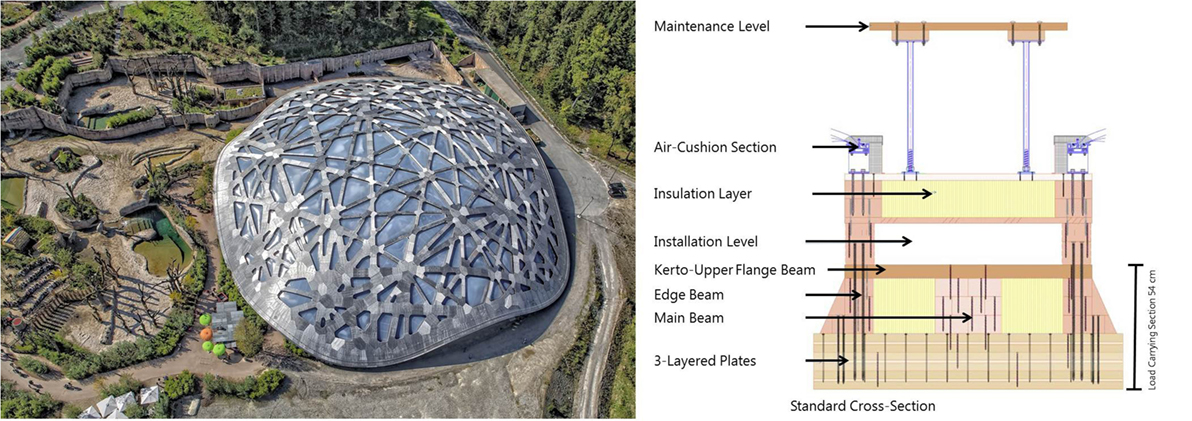
Figure 1. Left: aerial view of the structure (Gomez, 2015); right: cross-section of the timber roof.

2.2. Sensor Deployment and the Monitoring System

In collaboration with the engineers, numerous features have been monitored during the construction and operation phases via adoption of various instruments. The measurements were then analyzed and compared with the original design calculations. Albeit the measurements conducted during construction do not form the main concern of this paper, they do form part of the overall implemented SHM framework and as such, will be briefly elaborated upon herein. As observed in Figure 2, the post-tensioned ring beam is supported by a group of pillars, which comprise a permanent ground anchor carrying the horizontal shear forces from the shell to the ground. The displacement and rotation of these pillars were measured before and after this post-tensioning procedure via use of tachymeter and tiltmeter devices. Second, the vertical deflection of the roof was tracked as this was lowered from its temporary support structure (an extended system of steel scaffoldings) onto the ring beam, once again via use of tachymeters and appropriate mini reflector prisms (Figure 3 right). In addition to the prisms placed on the roof, a Rayleigh distributed fiber optic strain sensor was fixed to the roof beams in order to observe changes in strain with a spatial resolution of 10 mm, following several construction stages. Upon completion of the structure, short-term ambient vibration measurements were collected, in collaboration with the Swiss Seismological Service, by means of two broadband seismometers, placed on top of the roof and on top of the ring beam, respectively. The natural frequencies obtained through these ambient recordings were compared with the modal parameters predicted by the design model. A good correspondence was found between the observed quantities and the design variables (see Figure 3), increasing confidence in the design of this newly applied construction approach.

FIGURE 2

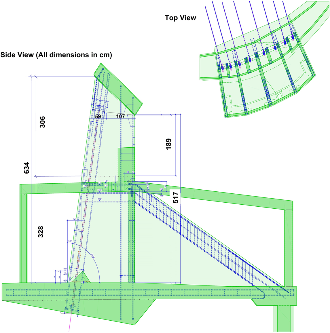
Figure 2. Top: plan view of a pillar group; left: cross-section and reinforcement drawing for a pillar.

FIGURE 3

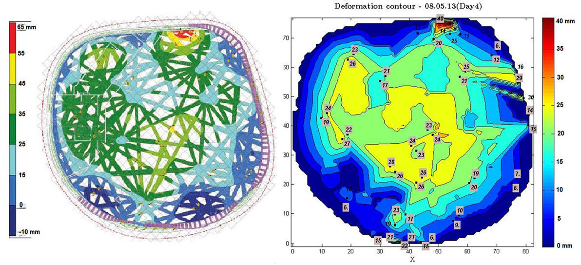
Figure 3. Deflection of the roof after lowering onto the ring beam. Left, calculated deflection; right, measured deflection.

The major, and essentially the only continuous, structural monitoring component of this deployment relies on the use of FBG strain sensors, which were embedded into 10 critical locations of the concrete ring beam. The sensors are attached to the steel reinforcement, by means of appropriate clamps, forming multiplexed chains of four sensors per section and serve the purpose of long-term monitoring of the strain evolution within critical post-tensioned concrete sections. Sections located at support points have been selected as the more critical ones, where direct feedback on strain was deemed as desirable. In addition to this installation, MAGEBA AG operates a permanent deployment of humidity sensors on the wooden cupola and temperature sensors on the outer and inner side of the structure. The deployed FBG sensors are Micronoptics embeddable os3600 strain sensors of a 20-cm active length. An example of such a sensor, mounted on reinforcement bars, is given in Figure 4, along with the sensor and DAQ unit locations. The nominal wavelength of each FBG strain sensor was selected specifically, so that no overlapping occurs within multiplexed chains when connected to the data acquisition unit (DAQ). The deployment of the sensors and the DAQ was performed in collaboration with MARMOTA AG and Smartec SA. Due to the harsh construction site conditions and the application of high-pressure self-compacting concrete, three of the embedded sensor chains, namely, the ones at locations F1, F3, and F9 were damaged. This is an inevitable reality when dealing with field deployments and, since embedded, the sensors may not be replaced after concreting. Nonetheless, the information offered by the currently operating system proves sufficient for the monitoring of structural condition, as elaborated in what follows. The sensors at each location are directed to the underground floor and subsequently collected via fiber optic cables at a central DAQ unit. Static strain readings are obtained using a 1-Hz sampling frequency and averaged every 5 min to transmit to an ftp-server shared and operated by MAGEBA AG. Although the models used herein are output-only, i.e., directly based on structural response measurements, a number of operational condition variables are additionally measured, namely, ambient temperature, humidity of the wooden roof, and force quantities for specific foundation anchorages. The complete set of these measurements is readily available to the client in a real-time manner through a graphical web interface. An additional feature of this system is that it works autonomously, meaning that data acquisition, processing, extraction of the condition indicator, and eventually notification of engineers for anomalies are achieved without any human interference through the execution of scripts in a pipeline fashion in regular intervals.

FIGURE 4

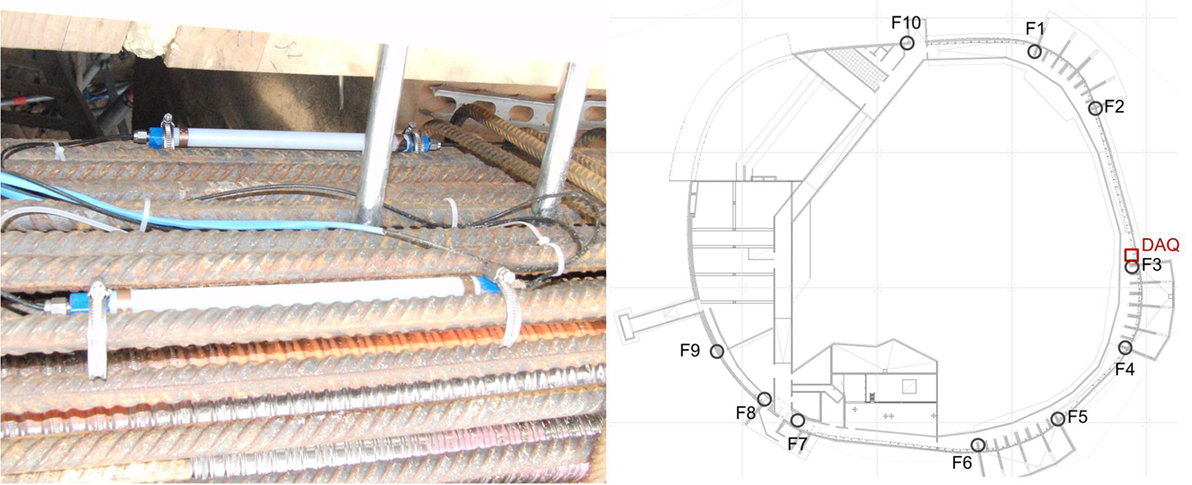
Figure 4. Left: permanent deployment of the Micronoptics embeddable FBG strain sensor os3600 on a reinforcement bar; right: technical drawing indicating the position of sensors and the DAQ.

The FBG measurement campaign initiated in April 2013, shortly before the post-tensioning of the ring tendons and has been ongoing ever since. The results of this early stage monitoring information are not presented further since they were not used to train and validate the automated “smart monitoring” framework, which is setup to run during the fully operational state. The period from September 2014 to March 2015 is herein reported, since the structure is primarily subjected to operational loads within this period and is free of other effects such as creep, shrinkage, post-tensioning, and intermittent loadings tied to sequential construction phases.

2.3. Basic Principles of FBG Sensing

As discussed earlier in Section 1, FBG-based strain sensors operate on the basis of the refractive properties of light and the reading and decoding of these refracted wavelengths (Merzbacher et al., 1996). Since the Bragg wavelength is affected both by mechanical and temperature influences, the total wavelength shift initially includes the mechanical and thermal strain that is induced on the monitored structure and the thermal strain induced on the sensor. One possibility to compensate such an effect relies on the use of a second parallel fiber that is only subjected to temperature change. A number of methods are already available for temperature compensation; the interested reader is referred to Majumder et al. (2008). The thermal strain of the fiber should therefore be compensated in order to obtain the true total strain, as specified by the following equation (MicronOptics, 2014):

${\mathrm{\epsilon }}_{\mathit{total}}\left[\mathrm{\mu \epsilon }\right]={10}^6\times \left[\frac{{\left(\mathrm{\Delta \lambda }∕{\mathrm{\lambda }}_0\right)}_S-{\left(\mathrm{\Delta \lambda }∕{\mathrm{\lambda }}_0\right)}_T}{F_G}\right]+\frac{{\left(\mathrm{\Delta \lambda }∕{\mathrm{\lambda }}_0\right)}_T}{S_T}\times \text{CT}{\text{E}}_T$ (1)

where,

• λ₀ is the zero measurement of strain or temperature sensing FBG,

• Δλ is the difference in wavelength in the strain or temperature sensing FBG with respect to the zero measurement,

• F_G, S_T, and CTE_T are constant values defined by the producers.

A related point to consider is that the abovementioned formula is based on theoretical derivations coupled with coefficients provided in the specifications of the manufacturer. For an optimal result, and provided time allows, every individual sensor should be tested a priori and their respective calibration coefficients ought to be determined in dedicated laboratory environments in ensuring a valid result interpretation. To such an end, Klug et al. (2014) report work on the calibration of SYLEX SC-01 FBG strain sensors for a monitoring project of expansion joints of a concrete arch dam for both temperature and strain. The calibration was conducted at the unique TU Graz fiber optic calibration facility (Presl, 2009). The authors would like to note such a rigorous calibration procedure was not feasible in this study, due to time pressure. Nonetheless, this further attests to the robustness of the developed monitoring scheme, since it additionally accounts for this discrepancy.

2.4. System Identification and Extraction of a Condition Indicator

The SHM methods adopted in this study exclusively rely on the tracking of the FBG strain response of the structure, rendering this an output-only scheme. This implies that environmental input parameters, such as ambient temperature and humidity, are not explicitly taken into account for identifying the structural model, although in fact measured. At this point, it is worth noting that in dense materials such as concrete, the thermal mass causes heat to be absorbed and released in the structure. This causes a lag (MPA, 2015) between the ambient and material temperature cycles, which could, in turn, cause problems in formulating an adequate regression model. As proven in what follows, this effect needs to be considered in deriving effective predictive models. A differentiation is therefore made between static and dynamic output-only methods on the basis of their “memory” on past structural response values.

Static methods assume that the input variables only have a short-time effect on structural behavior (Rajagopalan et al., 2012), whereas dynamic methods may account for the time evolution (history) of the response and operating conditions (Deraemaeker and Worden, 2012; Xia et al., 2015). It may be speculated in advance that a dynamic model is more suitable for the application investigated herein, since the heat stored within the concrete ring and humidity trapped in the wooden roof are non-negligible factors affecting structural response. However, for the sake of completeness, a static and dynamic output-only method is utilized, and their performance is compared with modeling and predicting the actual strain response of the structural system. The methods used within this context are the PCA and VAR models, which are briefly overviewed in the following sections.

2.4.1. Principal Component Analysis

Principle component analysis is a statistical technique used to project high-dimensional data sets of correlated observations onto compact coordinate systems, thus resulting in a smaller group of salient independent variables. If a set of N centered observations x_t ∈ ℝ and t = 1, …, N is considered to correspond to the measured structural responses from the FBG strain sensors at various locations of the concrete ring, the original data set x_t may be transformed into another set of m variables y_t as:

${\mathbf{\text{y}}}_t=T\times {\mathbf{\text{x}}}_t$ (2)

where T is a m-by-k orthonormal rotation matrix, used for transformation of the original coordinate system. The aforementioned rotation is materialized via solution of an eigenvalue problem, which results in estimation of a reduced number of principal components (Jolliffe, 2002). The principal components are extracted via diagonalization of the covariance matrix C, which reduces to an eigenvalue problem that is then solved by means of singular value decomposition:

$C=U\Sigma U^T$ (3)

Equation (3) can be factorized as follows by selecting the highest n₁ eigenvalues of Σ.

$C=\left[U_1{U}_2\right]\left[\begin{array}{cc}\hfill {\Sigma }_1\hfill & \hfill 0\hfill \\ \hfill 0\hfill & \hfill {\Sigma }_2\hfill \end{array}\right]\left[\begin{array}{c}\hfill U_1^T\hfill \\ \hfill U_2^T\hfill \end{array}\right]$ (4)

where Σ₁ denotes the submatrix of the highest n₁ eigenvalues, and U₁ is the matrix of corresponding eigenvectors. Finally, the orthonormal transformation of the original data can be achieved by setting T = U₁. The efficacy of the reduced projection may be validated by re-mapping the selected components of y_t back to the original domain, via use of the reduced matrix U₁ and its transpose as defined by the following equation:

${\widehat{\mathbf{\text{x}}}}_t=U_1{U}_1^T{\mathbf{\text{x}}}_t$ (5)

The remaining n₂ eigenvalues and corresponding eigenvectors U₂ may be employed to calculate the misfit of the projected values when compared against the original data. The residual error defined in equation (6) is adapted to this end, and herein serves as the PCA-based normalized condition indicator. The precision of the projection should be validated on a data set that is different to the one used for training.

${\mathbf{\text{e}}}_t=U_2{U}_2^T{\mathbf{\text{x}}}_t$ (6)

2.4.2. Vector AutoRegressive Models (VAR)

An extension to the univariate AutoRegressive model, VAR models are used for estimating a vector of current output variables on the basis of a string of past values. Equation (7) describes such a model.

${\mathbf{\text{x}}}_t+A_1{\mathbf{\text{x}}}_{t-1}+A_2{\mathbf{\text{x}}}_{t-2}+...+A_{n_a}{\mathbf{\text{x}}}_{t-n_a}=x_t+{\displaystyle \sum _{i=1}^{n_a}}{A}_i{\mathbf{\text{x}}}_{t-i}={\mathbf{\text{w}}}_t$ (7)

In equation (7), w_t is the vector series of independent identically distributed residual errors, which are assumed to follow a normal distribution with zero mean and a diagonal covariance matrix Σ_w, that is w_t ~ 𝒩(0, Σ_w). A_i with i = 1, 2, …, n_a, designate the Auto Regressive (AR) matrices, where n_a stands for the model order.

By means of ordinary least squares, the AR matrices may be straightforwardly estimated by reformulating the VAR model into a linear regression form. The model order may be n_a that can be selected by means of different criteria, such as the residual sum of squares and the Bayesian Information Criterion (BIC), which appropriately weigh on the model’s predictive capability (Lütkepohl, 2005).

The model’s one-step-ahead prediction is then obtained according to equation (8).

${\widehat{\mathbf{\text{x}}}}_{t|t-1}=-{\displaystyle \sum _{i=1}^{n_a}}{A}_i{\mathbf{\text{x}}}_{t-i}$ (8)

The prediction error of the VAR model, which here effectively serves as a normalized condition indicator, is given in equation (9) and coincides with the residual error w_t.

${\mathbf{\text{e}}}_t={\mathbf{\text{x}}}_t-{\widehat{\mathbf{\text{x}}}}_{t|t-1}$ (9)

As in the case of the PCA approach, the model is validated by implementation on a data set that is different to the one employed during the training phase.

It should be noted that for the indicators derived from both the PCA (residual error) and VAR (prediction error) schemes, efficacy is assessed on the basis of goodness of fit of the error distributions to a Gaussian-like distribution (with the Logistic distribution employed for the VAR case).

2.4.3. Robust Outlier Detection

Upon formulation of such indicators, a number of approaches may be implemented for outlier, or novelty, detection (Rousseeuw and Hubert, 2013). As elaborated upon in Dervilis et al. (2014, 2015), a classic discordancy measure used in the previous studies is the Mahalanobis squared-distance (MSD), which might, however, suffer from a multiple outlier “masking effect.” To this end, robust computation of location and covariance estimation of multivariate data may be exploited for investigation of inclusive outliers. The minimum covariance determinant (MCD) (Hubert and Debruyne, 2010) estimator or the minimum volume enclosing ellipsoid (MVEE) (Brunone et al., 2014) may be used in place of the MSD criterion for enhancing performance. Additionally, for indicators derived by means of time-series methods, such as the VAR approach employed herein, a number of statistical approaches for novelty detection are described in Fassois and Sakellariou (2007b), relying on the (a) the residual variance, (b) the residual uncorrelatedness, and (c) the likelihood function of the observed data, given the estimated state. These methods adopt formal statistical hypothesis testing procedures for establishing a threshold of a statistically significant deviation between the baseline (healthy) and current state. The abovementioned procedures are herein referenced for reasons of completeness toward a truly autonomous SHM framework, although they are so far not implemented for the “Kaeng Krachan” Elephant Shelter. As elaborated upon in the results section, the VAR model proves for now capable of fully describing the observed response, rendering minimal outliers. As data aggregate, the authors will cross-assess the previously listed outlier detection options for selecting the most appropriate to be implemented on the running SHM platform at the Zurich Zoo.

3. Results

The results presented herein overview implementation of both aforementioned models and performance is reported in terms of model prediction capabilities. Results are demonstrated for the second sensor from each chain at every location. These are denoted as x⋅2, where x denotes the sensor location. Sensors 1, 3, and 9 are excluded since data transmission is lost due to local effects, such as high-pressure concreting and cable damage. Figure 5 illustrates the measured strain time-series after the structure enters a fully operational state, starting from September 2014 until April 2015. It is evident that multiple gaps are present in the acquired series of data, relating to power shortages as well as various failures in the hardware/software of the measurement and data-logging equipment, an issue which is at this stage rectified. In order to side-step from any possible misfit, the estimation and validation sets are selected from time regions where constant data transmission has been achieved. The 1400 samples gathered in the period from December 2014 to January 2015 are herein used for training, whereas the 900 samples collected between February 2015 and March 2015 are utilized for validation.

FIGURE 5

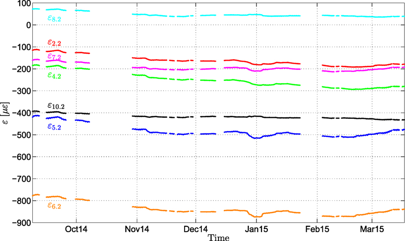
Figure 5. Strain evolution of the second sensor of each chain during the structure’s operational state.

3.1. Principal Component Analysis

In determining the number of principal components (PC) to maintain in the model, singular value decomposition is applied on the covariance matrix C of the estimation set, with the resulting normalized eigenvalues and their respective percentage of explained variance plotted in Figure 6. As observed in that figure, the first and second PC explain 89 and 10.52% of the variance, respectively; thus, already the first two eigenvalues capture more than 99.5% of the variance characterizing the available strain measurements. The remaining PCs do not bear a significant effect and are thus neglected in the adopted PCA model.

FIGURE 6

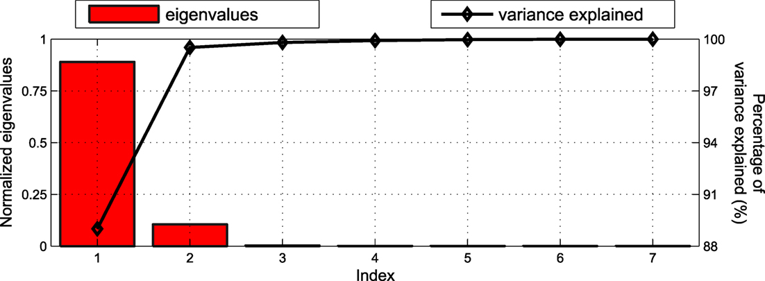
Figure 6. Normalized eigenvalues and percentage of explained variance of the estimation set.

By retaining only the first two principal components, the original data are projected onto the PC space domain and the projection of both the estimation and the validation set is illustrated in Figure 7. It is observed that the PCA projection is able to follow the manifested trend at all sensor locations; however, the details are not very well tracked. These details are attributed to daily fluctuations in temperature, humidity, wind, and other environmental factors, and the ability to follow these may prove of utmost importance for a monitoring framework. The top plot in Figure 8 illustrates the prediction error for sensor F2, for both the estimation and validation data sets, along with the corresponding distributions. The mean squared prediction error (MSPE) of the validation set, for each sensor, is calculated as F₂: 0.7513, F₄: 0.1383, F₅: 0.4185, F₆: 0.3096, F₇: 0.1471, F₈: 0.3900, and F₁₀: 1.4162. As observed in Figure 8, the estimation and validation set prediction error seems to follow no specific distribution. The lack of a Gaussian-like distribution indicates that the PCA approach does not yield a suitable condition/damage index that is informative of structural performance.

FIGURE 7

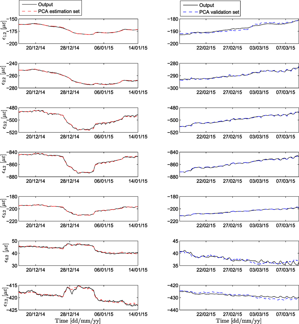
Figure 7. PCA model performance in modeling strain for the estimation and validation data sets.

FIGURE 8

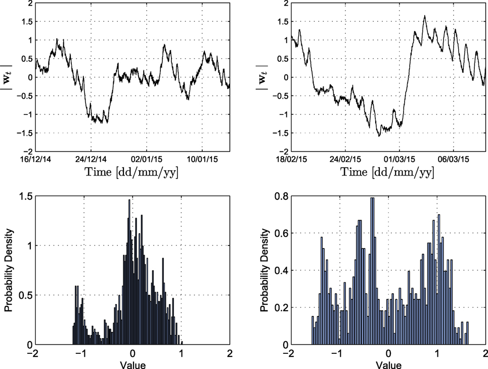
Figure 8. Top: PCA prediction error for the estimation (left) and validation set (right) of sensor F2. Bottom: histograms of the prediction error for each set.

3.2. Vector Autoregressive Models

The order of the VAR model is selected on the basis of the BIC. As observed in Figure 9, the BIC value stabilizes after a model order of 10 and therefore this is retained as the implemented order of the VAR model. A higher model order would not yield an improved prediction at the cost of incurring an additional burden on computation. The one-step-ahead prediction performance of a VAR (10) model is illustrated in Figure 10 both for the estimation and validation data sets. Due to the dynamic nature and inherent memory of this modeling approach, the daily fluctuations of the signal, discussed in the previous section, are now adequately captured. The MATLAB function “allfitdist” is utilized for fitting a multitude of probabilistic distributions to the prediction error data set, and the BIC is then employed to return the optimal fit (Mathworks, 1998; Sheppard, 2012). The prediction error time histories, again for the monitored strains of sensor F2, and their corresponding distributions are plotted in Figure 11 for both the estimation and validation set. The mean squared prediction error (MSPE) of the validation set, for each sensor, results significantly lower to the PCA equivalent, namely F₂: 0.0050, F₄: 0.0062, F₅: 0.0179, F₆: 0.0167, F₇: 0.0280, F₈: 0.0086, and F₁₀: 0.0147. As observed therein, the prediction error of VAR (10) follows a Logistic distribution with a location parameter that results very close to zero. The distribution parameters are Logistic (−1.44 × 10⁻⁴, 0.16) for the estimation and Logistic (−0.21, 0.18) for the validation set. Given the fact that the Logistic distribution closely resembles a Gaussian distribution, only with a higher kurtosis (Johnson et al., 1995), it is concluded that the FBG strain measurements are adequately predicted by means of the VAR (10) model and the calculated error norm may be employed as a condition indicator within the proposed output-only continuous monitoring framework.

FIGURE 9

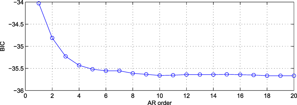
Figure 9. Evolution of the Bayesian information criterion (BIC) for increasing model order.

FIGURE 10

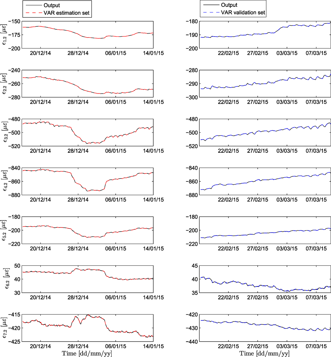
Figure 10. VAR model performance in modeling strain for the estimation and validation data-sets.

FIGURE 11

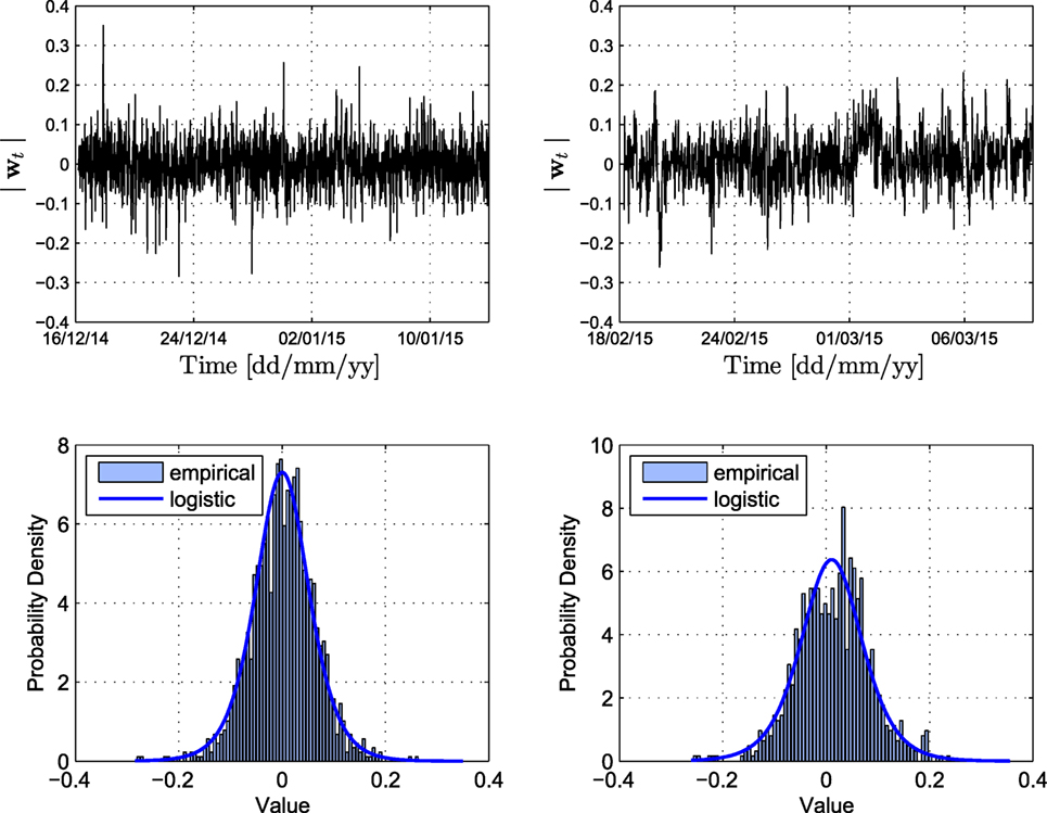
Figure 11. Top: VAR prediction error for the estimation (left) and validation set (right) of sensor F2. Bottom: histograms and fitted distribution of the prediction error for each set.

4. Discussion

This work presents an implementation of an autonomous monitoring scheme on a novel 80 m span wooden free-form cupola, supported by a post-tensioned RC beam. The long-term monitoring campaign was planned and organized in collaboration with the owner and design engineers. This study overviews the set of methods and tools adopted, as well as the interpretation of the acquired data streams into effective metrics for assessing structural performance.

• To this end, FBG strain sensors were embedded into critical locations in the post-tensioned RC ring, continually transferring information regarding structural condition.

• In efficiently handling this data, and for doing so in real-time, two output-only models are investigated herein. The goal is to come up with the so-called normalized condition indicators, able to warn of anomalies or irregular behavior in support of inspection/maintenance strategies.

• A static (PCA) and a dynamic (VAR) model are implemented, revealing superiority of the VAR-type model, which may be attributed to its inherent feature of memory. Once an adequate model (predictor) is formulated on the basis of a training data-set, the prediction error may be employed as a condition indicator.

• In this early stage, the goodness of fit of the error distribution in respect to a Logistic distribution is used to assess whether response remains within regular limits. When further data are aggregated, delivering more instances of outliers, more refined outlier detection schemes will be investigated and accordingly adopted.

Condition indicators of this form, extracted from automated monitoring tools, may subsequently be coupled with standard inspection schemes (e.g., visual inspection) in support of decision-making processes. To this end, a number of tools exist able to exploit information on the system’s state, which itself comprises a stochastic variable, with a set of possible actions and observations for optimally managing infrastructure assets. The interested reader is referred to Straub and Faber (2005), Kim et al. (2013), May et al. (2015), and Schöbi and Chatzi (2015). In a next stage, the potential for damage localization will be explored by exploiting the spatial distribution of the sensors along the ring. This study reports the early results of an actual monitoring campaign, aiming to serve as a reference for the fusion of data acquisition techniques and appropriate processing tools toward smart infrastructure management.

Author Contributions

All authors listed, have made substantial, direct and intellectual contribution to the work, and approved it for publication.

Conflict of Interest Statement

The authors declare that the research was conducted in the absence of any commercial or financial relationships that could be construed as a potential conflict of interest.

Acknowledgments

The authors would like to acknowledge the following groups/entities and gratefully thank them for their contributions: Zoo Zürich AG, Walt + Galmarini AG, MAGEBA AG, Marmota AG, the IBK-Lab staff, and the further colleagues from the Chair of Structural Mechanics of ETH Zürich, who assisted in materializing this deployment. This research has been financially supported by the Zoo Zürich AG and the Albert Lück-Stiftung.

Nomenclature

Δ	Shift in a certain value, e.g., temperature, Bragg wavelength, etc.
λ0	Initial (Zero) Bragg wavelength
Σ	Diagonal submatrix containing eigenvalues
ε	Strain measured by FBG sensors
xt	Observed quantities (measurements)
yt	Transformed quantities in PCA
C	Covariance matrix (PCA)
CTE	Coefficient of Thermal Expansion
e	Prediction error
N	Number of observations
T	Orthonormal rotation matrix
U	Eigenvectors

References

Aktan, A. E., Farhey, D. N., Helmicki, A. J., Brown, D. L., Hunt, V. J., Lee, K.-L., et al. (1997). Structural identification for condition assessment: experimental arts. J. Struct. Eng. 123, 1674–1684. doi: 10.1061/(ASCE)0733-9445(1997)123:12(1674)

CrossRef Full Text | Google Scholar

Bornn, L., Farrar, C. R., Park, G., and Farinholt, K. (2009). Structural health monitoring with autoregressive support vector machines. J. Vib. Acoust. 131, 21004. doi:10.1115/1.3025827

CrossRef Full Text | Google Scholar

Brownjohn, J. M. (2007). Structural health monitoring of civil infrastructure. Philos. Trans. Roy. Soc. Lond. A Math. Phys. Eng. Sci. 365, 589–622. doi:10.1098/rsta.2006.1925

CrossRef Full Text | Google Scholar

Brunone, B., Giustolisi, O., Ferrante, M., Laucelli, D., Meniconi, S., Berardi, L., et al. (2014). 12th International conference on computing and control for the water industry, ccwi2013 minimum volume ellipsoid classification model for contamination event detection in water distribution systems. Proc. Eng. 70, 1280–1288. doi:10.1016/j.proeng.2014.02.141

CrossRef Full Text | Google Scholar

Casas, J., and Cruz, P. (2003). Fiber optic sensors for bridge monitoring. J. Bridge Eng. 8, 362–373; Special issue: bridge management systems. doi:10.1061/(ASCE)1084-0702(2003)8:6(362)

CrossRef Full Text | Google Scholar

Catbas, F. N., and Aktan, A. E. (2002). Condition and damage assessment: issues and some promising indices. J. Struct. Eng. 128, 1026–1036. doi:10.1061/(ASCE)0733-9445(2002)128:8(1026)

CrossRef Full Text | Google Scholar

Chan, T. H., Yu, L., Tam, H. Y., Ni, Y. Q., Liu, S. Y., and Chung, W. H. (2006). Fiber Bragg grating sensors for structural health monitoring of Tsing Ma Bridge: background and experimental observation. Eng. Struct. 28, 648–659. doi:10.1016/j.engstruct.2005.09.018

CrossRef Full Text | Google Scholar

Chatzi, E., and Spiridonakos, M. (2015). “Dealing with uncertainty in the monitoring and simulation of dynamically evolving systems,” in Proceedings of the 7th International conference on Structural Health Monitoring of Intelligent Infrastructure (SHM-II) (Torino, Italy).

Google Scholar

Deraemaeker, A., and Worden, K. (2012). New Trends in Vibration Based Structural Health Monitoring, Vol. 520. Wien: Springer Science & Business Media.

Google Scholar

Dervilis, N., Cross, E., Barthorpe, R., and Worden, K. (2014). Robust methods of inclusive outlier analysis for structural health monitoring. J. Sound Vibrat. 333, 5181–5195. doi:10.1016/j.jsv.2014.05.012

CrossRef Full Text | Google Scholar

Dervilis, N., Worden, K., and Cross, E. (2015). On robust regression analysis as a means of exploring environmental and operational conditions for {SHM} data. J. Sound Vibrat. 347, 279–296. doi:10.1016/j.jsv.2015.02.039

CrossRef Full Text | Google Scholar

Elgamal, A., Conte, J., Masri, S., Fraser, M., Fountain, T., Gupta, A., et al. (2003). “Health monitoring framework for bridges and civil infrastructure,” in Proceedings of the 4th International Workshop on Structural Health Monitoring (Structures And Composites Laboratory (SACL) in the Department of Aeronautics & Astronautics at Stanford University), 123–130.

Google Scholar

Farrar, C. R., and Worden, K. (2007). An introduction to structural health monitoring. Philos. Trans. Roy. Soc. Lond. A Math. Phys. Eng. Sci. 365, 303–315. doi:10.1098/rsta.2006.1928

CrossRef Full Text | Google Scholar

Fassois, S. D., and Kopsaftopoulos, F. P. (2013). Statistical Time Series Methods for Vibration Based Structural Health Monitoring. Vienna: Springer, 209–264.

Google Scholar

Fassois, S. D., and Sakellariou, J. S. (2007a). Time-series methods for fault detection and identification in vibrating structures. Philos. Trans. Roy. Soc. A 365, 411–448. doi:10.1098/rsta.2006.1929

CrossRef Full Text | Google Scholar

Fassois, S. D., and Sakellariou, J. S. (2007b). Time-series methods for fault detection and identification in vibrating structures. Philos. Trans. Roy. Soc. Lond. A Math. Phys. Eng. Sci. 365, 411–448. doi:10.1098/rsta.2006.1929

CrossRef Full Text | Google Scholar

Fuhr, P. L., and Huston, D. R. (1993). Multiplexed fiber optic pressure and vibration sensors for hydroelectric dam monitoring. Smart Mater. Struct. 2, 260. doi:10.1088/0964-1726/2/4/008

CrossRef Full Text | Google Scholar

Gomez, R. (2015). in Kaeng krachan elefantenpark aus der luft, ed. A. G. Sika Schweiz (Zurich, Switzerland). Accessed via zoo.ch, 01.12.2015.

Google Scholar

Hubert, M., and Debruyne, M. (2010). Minimum covariance determinant. Wiley Inter. Rev. Comput. Stat. 2, 36–43. doi:10.1002/wics.61

CrossRef Full Text | Google Scholar

Johnson, N. L., Kotz, S., and Balakrishnan, N. (1995). Continuous Univariate Distributions, Vol. 2. Hoboken, NJ: Wiley & Sons.

Google Scholar

Jolliffe, I. (2002). Principal Component Analysis. Encyclopedia of Statistics in Behavioral Science. Wiley Online Library.

Google Scholar

Kim, S., Frangopol, D. M., and Soliman, M. (2013). Generalized probabilistic framework for optimum inspection and maintenance planning. J. Struct. Eng. 139, 435–447. doi:10.1061/(ASCE)ST.1943-541X.0000676

CrossRef Full Text | Google Scholar

Klug, F., Lienhart, W., and Woschitz, H. (2014). “High resolution monitoring of expansion joints of a concrete arch dam using fiber optic sensors,” in Proc. 6th World Conference on Structural Control and Monitoring (6WCSCM) (Barcelona: Universitat Politècnica de Catalunya (UPC)), 3164–3176.

Google Scholar

Klug, F., and Woschitz, H. (2015). “Test and calibration of 20 fbg based strain transducers,” in Proc. Machine Vision Applications VIII, SPIE, Vol. 9405. San Francisco.

Google Scholar

Kreuzer, M. (2006). Strain Measurement with Fiber Bragg Grating Sensors. Darmstadt: HBM, S2338.

Google Scholar

Kronenberg, P., Casanova, N., Inaudi, D., and Vurpillot, S. (1997). “Dam monitoring with fiber optics deformation sensors,” in Smart Structures and Materials’ 97 (San Diego: International Society for Optics and Photonics), 2–11.

Google Scholar

Lee, H., and Sohn, H. (2012). Damage detection for pipeline structures using optic-based active sensing. Smart Struct. Syst. 9, 461–472. doi:10.12989/sss.2012.9.5.461

CrossRef Full Text | Google Scholar

Lee, W., Lee, W.-J., Lee, S.-B., and Salgado, R. (2004). Measurement of pile load transfer using the fiber Bragg grating sensor system. Can. Geotech. J. 41, 1222–1232. doi:10.1139/t04-059

CrossRef Full Text | Google Scholar

Li, H.-N., Li, D.-S., and Song, G.-B. (2004). Recent applications of fiber optic sensors to health monitoring in civil engineering. Eng. Struct. 26, 1647–1657. doi:10.1016/j.engstruct.2004.05.018

CrossRef Full Text | Google Scholar

Lütkepohl, H. (2005). New Introduction to Multiple Time Series Analysis. Berlin, Heidelberg: Springer.

Google Scholar

Majumder, M., Gangopadhyay, T., Chakraborty, A., Dasgupta, K., and Bhattacharya, D. (2008). Fibre Bragg gratings in structural health monitoring – present status and applications. Sens. Actuators A Phys. 147, 150–164. doi:10.1016/j.sna.2008.04.008

CrossRef Full Text | Google Scholar

Mathworks, T. (1998). Matlab User’s Guide Inc, Vol. 5. (Natick, MA: Mathworks GmbH, Murtenstrasse, 3008 Bern), 333.

Google Scholar

May, A., McMillan, D., and Thöns, S. (2015). “Integrating structural health and condition monitoring: a cost benefit analysis for offshore wind energy,” in ASME 2015 34th International Conference on Ocean, Offshore and Arctic Engineering (St. John’s: American Society of Mechanical Engineers), A57–A59.

Google Scholar

Merzbacher, C., Kersey, A., and Friebele, E. (1996). Fiber optic sensors in concrete structures: a review. Smart Mater. Struct. 5, 196–208. doi:10.1088/0964-1726/5/2/008

CrossRef Full Text | Google Scholar

MicronOptics. (2014). Technical Note 1025, Revision 2014.1.31.1 – Fbg Total Strain Sensor Thermal Considerations: Five Steps to Meaningful Strain Data. Technical report. Atlanta, GA: MicronOptics.

Google Scholar

Moore, J., Gischig, V., Button, E., and Loew, S. (2010). Rockslide deformation monitoring with fiber optic strain sensors. Nat. Hazards Earth Syst. Sci. 10, 191. doi:10.5194/nhess-10-191-2010

CrossRef Full Text | Google Scholar

MPA. (2015). “Thermal mass explained,” in The Concrete Centre. Available at: http://www.concretecentre.com/technical_information/performance_and_benefits/thermal_mass.aspx

Google Scholar

Nandan, H., and Singh, M. (2011). “Civil engineering topics,” in Part of the series Conference Proceedings of the Society for Experimental Mechanics Series, Vol. 4 (Springer), 273–284.

Google Scholar

Nguyen, V. H., Mahowald, J., Golinval, J.-C., and Maas, S. (2014a). “Damage detection in bridge structures including environmental effects,” in The Ninth International Conference on Structural Dynamics EURODYN 2014, Porto.

Google Scholar

Nguyen, V. H., Mahowald, J., Golinval, J.-C., and Maas, S. (2014b). “Damage detection in civil engineering structure considering temperature effect,” in Dynamics of Civil Structures, Vol. 4 (Orlando: Springer), 187–196.

Google Scholar

Peeters, B., and De Roeck, G. (2001). One-year monitoring of the z 24-bridge: environmental effects versus damage events. Earthquake Eng. Struct. Dynam. 30, 149–171. doi:10.1002/1096-9845(200102)30:2<149::AID-EQE1>3.0.CO;2-Z

CrossRef Full Text | Google Scholar

Peeters, B., Maeck, J., and De Roeck, G. (2001). Vibration-based damage detection in civil engineering: excitation sources and temperature effects. Smart Mater. Struct. 10, 518. doi:10.1088/0964-1726/10/3/314

CrossRef Full Text | Google Scholar

Presl, R. (2009). Entwicklung eines automatisierten messsystems zur charakterisierung faseroptischer dehnungssensoren. Master thesis, FH Oberösterreich, Oberösterreich.

Google Scholar

Rajagopalan, V., Behera, A., Bhattacharya, A., Prabhu, R., and Badami, V. (2012). “Estimation of static deflection under operational conditions for blade health monitoring,” in Prognostics and System Health Management (PHM), 2012 IEEE Conference on (Beijing: IEEE), 1–6.

Google Scholar

Rice, J. A., Mechitov, K., Sim, S.-H., Nagayama, T., Jang, S., Kim, R., et al. (2010). Flexible smart sensor framework for autonomous structural health monitoring. Smart Struct. Syst. 6, 423–438. doi:10.12989/sss.2010.6.5_6.423

CrossRef Full Text | Google Scholar

Robert-Nicoud, Y., Raphael, B., Burdet, O., and Smith, I. (2005). Model identification of bridges using measurement data. Comput. Aided Civ. Infrastruct. Eng. 20, 118–131. doi:10.1111/j.1467-8667.2005.00381.x

CrossRef Full Text | Google Scholar

Rousseeuw, P., and Hubert, M. (2013). High-Breakdown Estimators of Multivariate Location and Scatter, Chap. 4. Berlin, Heidelberg: Springer, 49–66.

Google Scholar

Sazonov, E., Janoyan, K., and Jha, R. (2004). “Wireless intelligent sensor network for autonomous structural health monitoring,” in Smart Structures and Materials (San Diego, CA: International Society for Optics and Photonics), 305–314.

Google Scholar

Schmidt-Hattenberger, C., Straub, T., Naumann, M., Borm, G., Lauerer, R., Beck, C., et al. (2003). “Strain measurements by fiber Bragg grating sensors for in situ pile loading tests,” in Smart Structures and Materials (San Diego, CA: International Society for Optics and Photonics), 289–294.

Google Scholar

Schöbi, R., and Chatzi, E. N. (2015). Maintenance planning using continuous-state partially observable Markov decision processes and non-linear action models. Struct. Infrastruct. Eng. 12, 1–18. doi:10.1080/15732479.2015.1076485

CrossRef Full Text | Google Scholar

Sheppard, M. (2012). “Fit all valid parametric probability distributions to data,” in Mathworks File Exchange (Mathworks). Available at: http://www.mathworks. com/matlabcentral/fileexchange/34943-fit-all-valid-parametric-probability-distributions-to-data

Google Scholar

Sohn, H. (2007). Effects of environmental and operational variability on structural health monitoring. Philos. Trans. Roy. Soc. Lond. A Math. Phys. Eng. Sci. 365, 539–560. doi:10.1098/rsta.2006.1935

CrossRef Full Text | Google Scholar

Spiridonakos, M., and Chatzi, E. (2014a). “Polynomial chaos expansion models for SHM under environmental variability,” in Proceedings of Eurodyn 2014, 9th International Conference on Structural Dynamics (Porto, Portugal).

Google Scholar

Spiridonakos, M., and Chatzi, E. (2014b). “Stochastic structural identification from vibrational and environmental data,” in Encyclopedia of Earthquake Engineering: SpringerReference (Berlin, Heidelberg: Springer-Verlag), 1–16.

Google Scholar

Spiridonakos, M., Chatzi, E., and Sudret, B. (2016). Polynomial chaos expansion models for the monitoring of structures under operational variability. ASCE-ASME J. Risk Uncertainty Eng. Syst., Part A: Civ. Eng.. doi:10.1061/AJRUA6.0000872

CrossRef Full Text | Google Scholar

Straub, D., and Faber, M. H. (2005). Risk based inspection planning for structural systems. Struct. Saf. 27, 335–355. doi:10.1016/j.strusafe.2005.04.001

CrossRef Full Text | Google Scholar

Tennyson, R., Mufti, A., Rizkalla, S., Tadros, G., and Benmokrane, B. (2001). Structural health monitoring of innovative bridges in Canada with fiber optic sensors. Smart Mater. Struct. 10, 560. doi:10.1088/0964-1726/10/3/320

CrossRef Full Text | Google Scholar

Wenzel, H. (2009). “The influence of environmental factors,” in Encyclopedia of Structural Health Monitoring. Wiley Online Library.

Google Scholar

Worden, K., and Dulieu-Barton, J. (2004). An overview of intelligent fault detection in systems and structures. Struct. Health Monitor. 3, 85–98. doi:10.1177/1475921704041866

CrossRef Full Text | Google Scholar

Xia, L., Yu, C., Ran, Y., Xu, J., and Li, W. (2015). Static/dynamic strain sensing applications by monitoring the correlation peak from optical wideband chaos. Opt. Express 23, 26113–26123. doi:10.1364/OE.23.026113

CrossRef Full Text | Google Scholar

Yan, A.-M., Kerschen, G., De Boe, P., and Golinval, J.-C. (2005). Structural damage diagnosis under varying environmental conditions – part I: a linear analysis. Mech. Syst. Signal Process. 19, 847–864. doi:10.1016/j.ymssp.2004.12.003

CrossRef Full Text | Google Scholar

Yuen, K.-V., and Kuok, S.-C. (2010). Ambient interference in long-term monitoring of buildings. Eng. Struct. 32, 2379–2386. doi:10.1016/j.engstruct.2010.04.012

CrossRef Full Text | Google Scholar

Zoo-Zürich. (2014). More Room for the Biggest Animals. Available at: http://www.zoo.ch/xml_1/internet/en/application/d693/f2619.cfm

Google Scholar