Optimizing Urban Bus Transit Network Design Can Lead to Greenhouse Gas Emissions Reduction

Introduction

With the increasing concern about global climate change, greenhouse gas (GHG) emission levels of the transportation sector have gained significant interest among researchers and policy makers. Transportation contributes 28% of all greenhouse gas emissions in the United States and 23% worldwide (Kahn Ribeiro et al., 2007; Environmental Protection Agency, 2014). Most efforts to mitigate GHG emissions from transit have focused on vehicle technology and mode shifts from private automobile (Gallivan and Grant, 2010). Technological approaches, retrofitting engines, or replacing vehicles, can be expensive, while increasing transit service to attract drivers to the system can backfire and cause a net increase in emissions (Poudenx, 2008). Public transit systems that operate with low ridership have been shown to have higher per-passenger-kilometer emissions than the automobile (Chester and Horvath, 2009).

Griswold et al. (2013) took a different approach by incorporating emissions constraints into continuum approximation (CA) models that traditionally have only accounted for costs. They minimized costs subject to a GHG emissions constraint, and by varying the constraint, established the Pareto frontier of optimal system design, allowing them to examine the tradeoff between costs and emissions. A disadvantage of this approach is that any reductions in GHG emissions below the cost-optimal level come with a penalty in increased user travel time, which could send users to more polluting modes.

Existing transit systems are not designed to optimize for costs, so it is likely that most systems are operating above the Pareto frontier, with both higher costs and emissions. This paper addresses the unexplored question of how much GHG emissions can be reduced by moving an existing transit system to the cost-optimal point on the Pareto curve. Unlike the emissions reductions identified in Griswold et al. (2013), there is theoretically no cost associated with these reductions. Barcelona provides an excellent case study as a city for which a cost-optimal transit system has already been designed, requiring only the addition of emissions estimates. Daganzo (2010) designed a transit system for Barcelona to be competitive with automobile in terms of travel time.

Much of the literature related to transit emissions focuses on operating emissions and does not account for total life-cycle emissions (Herndon et al., 2005; Puchalsky, 2005). This paper includes life-cycle GHG emissions that relate to infrastructure, maintenance, and vehicle manufacturing and operations, using emissions parameters estimated by Chester and Horvath (2009).

In this paper, we estimate the level of GHG emission reductions that can occur as a result of designing a transit network for optimal societal costs. We hypothesize that user and agency costs are minimized in the design of a network, both costs and GHG emissions will be reduced. The following section describes the CA methods that are used to develop a model of the transit network to optimize. Section “Case Study Findings” present the case study findings and section “Conclusion” concludes with discussion of limitations and future work.

Transit Network Optimization

Continuum approximation methods have been developed and utilized in order to optimize transit networks with the objective of minimizing user and agency costs. That is, minimizing the time spent by users accessing, waiting, transferring, and riding (and the corresponding costs associated with these times) and the costs required to maintain and operate the system. CA methods provide decision makers with insights on optimal system design by making generalizations that simplify the analysis. Utilizing CA models yields decision variables that can be implemented in design, such as stop spacing, service frequencies (headways), and line spacing. Of course, the generated decision variables may need to be slightly modified in order to appropriately fit geographic and pre-existing infrastructure conditions of the design region. The need for these adjustments will be discussed further in the following section.

There has been a variety of work examining different transit network structures. While Holroyd (1967) looks at grids, Byrne (1975) radial systems, and Newell (1979) hub-and-spoke systems, Daganzo (2010) makes a crucial advancement toward making transit networks more competitive with the private automobile by developing a hybrid structure. Utilizing this design, a system may have a grid structure in the center of the city where demand densities are higher and a hub-and-spoke network on the peripheries, thereby more efficiently utilizing resources and matching a city’s demand. With some adjustments, this model is utilized by Estrada et al. (2011) in order to design an efficient, feasible transit network for the city of Barcelona. The results of this optimization serve as the inputs for our cost and GHG emission analysis that is presented in the following section.

Equation 1, below, and those in the Section “Mathematical Program for Network Optimization” in Appendix were developed by Daganzo (2010) and modified by Estrada et al. (2011) in order to optimize the transit network system in Barcelona. Figure 1 shows the simplified structure of the model used by Estrada et al. (2011). A rectangular grid of dimensions d_x by d_y sits within a larger rectangle of dimensions D_x by D_y. The outer part of the rectangle contains the hub-and-spoke design. The decision variables relating these dimensions are α_x = d_x/D_x and α_y = d_y/D_y. Furthermore, in the Barcelona analysis, these two values were assumed to be equal and, therefore, collapsed into one decision variable, α. The stop spacings are represented by s_x and s_y. Utilizing the aforementioned CA methods, an objective function was developed based on total system costs. This was minimized subject to a number of constraints including the maximum number of allowable corridors and the minimum headways, H (3 min). The objective function displayed below is comprised of two major components: agency costs and user costs.

$\begin{array}{l}\hfill \text{min\hspace{0.17em}}{Z}_{\text{system}}=\left[{\mathrm{\pi }}_V\ast V+{\mathrm{\pi }}_M\ast M+{\mathrm{\pi }}_L\ast L\right]+\left[A+W+T+\left(\frac{\mathrm{\delta }}{v_w}\right)\ast e_T\right]\end{array}$ (1)

FIGURE 1

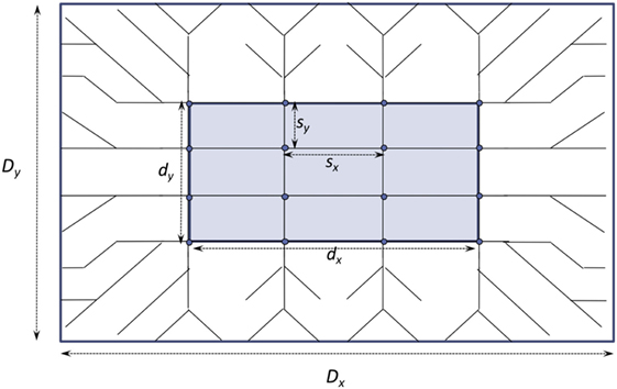
Figure 1. The extension of Daganzo (2010) hybrid structure used by Estrada et al. (2011) when designing Barcelona’s optimized transit network.

As was previously mentioned, the objective function in Eq. 1 was minimized subject to headway, corridor, occupancy, and other geometric constraints. The full mathematical program and all of the variable calculations can be found in the Section “Mathematical Program for Network Optimization” in Appendix. In the first set of brackets of the objective function are the agency costs, comprising vehicle-km/h traveled V, the maximum number of buses required in the fleet during peak hours M, and the one-way infrastructure length L. Each of these components are multiplied by a corresponding factor π_i that ensures the objective function is in units of time and utilizes proper wage rates. The second bracket in the objective function corresponds to the user cost. This cost is again measured in time spent by the average user in the system. It is composed of the access and egress time A, the waiting time W, the in-vehicle travel time T, and the equivalent time cost of transferring buses. This last term is made up of a ratio between some constant δ (hr) and the walking speed v_w (km/hr) multiplied by the expected transfer value e_T. The model was optimized and decision variables were obtained: α = 0.85, s = 0.65 km, H = 3 min. These values laid a foundation for a model that was slightly modified and is discussed below. The following section discusses how these values were utilized in a case study design and compares the total costs and GHG emissions between the current system and the proposed design.

Case Study Findings

In this section, we will present our findings regarding the change in both cost and GHG emissions that can result when optimizing a transit network. Specifically, we will be looking at a case study of Barcelona. First, we present the parameters that were determined by Estrada et al. (2011) when optimizing the bus network. Second, we will present our analysis of both costs and GHG reductions that result. The significance of this particular case study is of interest as Barcelona is representative of many cities worldwide. Its rectangular shape is shared by many cities, e.g., New York, Beijing, and Abu Dhabi, and, therefore, similar analysis presented in this paper can be easily extrapolated. Furthermore, the high transit ridership and significance of the bus share in Barcelona suggest relevance in our analysis and findings. Finally, comprehensive information regarding the modeling of an efficient design is available for Barcelona, primarily due to the work developed by Estrada et al. (2011).

The Barcelona optimization model employed by Estrada et al. (2011) expands upon Daganzo’s (2010) aforementioned hybrid structure. Constraints were used that represented several limiting factors including the number of available corridors and minimum allowable headways. An objective function composed of average agency and user costs was optimized in order to determine optimal stop spacing, line spacing, and headways. The model yielded analytic results that were then adjusted in order to fit Barcelona in actuality, that is, taking into consideration the layout of the city, modifying routes to serve universities, hospitals, and other demand centers. The resulting model yielded information regarding traveler level of service as well as infrastructure and fleet size values. Table 1 presents highlights of the model developed by Estrada et al. (2011) and the cost comparisons between its corresponding values and those of the current system.

TABLE 1

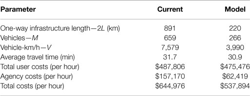
Table 1. Current and modeled design parameters and corresponding costs of Barcelona network (Estrada et al., 2011).

The optimization and design modification described above produce a 17% reduction in costs from the current system to the proposed model. Detailed cost calculations can be found in the Section “Cost Calculations” in Appendix. The majority of the reduction is carried by the agency. That is, the unsubsidized fare would be lower in the proposed design. It should be noted that in this case the average travel time remained very similar (with a 2.5% difference) and, therefore, it is reasonable to assume that no mode shifts would be expected due to travel time changes. In other applications, this may not be the case and should be taken into consideration. From the above table, it is clear that optimizing a transit network has the potential to reduce costs significantly. In our analysis, we explore how this optimization affects GHG emissions.

While much effort in understanding transportation-related GHG emissions has typically been placed on tailpipe emissions, we are focused on life-cycle emissions associated with each of the aforementioned scenarios. Utilizing the emissions parameters developed by Chester and Horvath (2009), we were able to calculate and compare the model-based design GHG emissions with the emissions of the existing network in Barcelona. As formulated in Eq. 2, the life-cycle assessment includes not only operating emissions, but emissions from vehicle manufacturing, system maintenance, and infrastructure construction as well. Inputting network characteristics, we utilized the following equation to relate infrastructure length 2L, number of vehicles M, and vehicle-km/h V with the corresponding hourly GHG emission levels. The details of the parameters used in Eq. 2 are presented in Table 2. It should be noted that in our analysis emission levels are solely related to agency attributes. This is because users are assumed to be accessing the system exclusively by walking and are, therefore, not contributing additional emissions.

$\text{Emissions\hspace{0.17em}}\left(\text{C}{\text{O}}_{\text{2}}\text{e\hspace{0.17em}g/h}\right)=E_I\ast 2L+E_M\ast M+E_V\ast V$ (2)

TABLE 2

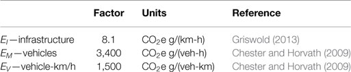
Table 2. Emission factors.

The optimized model yields a network that produces much lower GHG emissions than the current network (Table 3). The infrastructure component takes into consideration the shared use of buses and automobiles on the road. Furthermore, in our calculations, we did not include bus stop infrastructure emissions as they are negligible when compared to the other components. This assumption should not be made if further work is performed on systems including modes such as rail, where station construction contributes to high levels of GHG emissions (Chester, 2008). The discussion of the effects of the station construction emissions is found in Griswold et al. (2013). The emission factor corresponding to the vehicles assumes an average usage length of 8 years. This duration is based on Barcelona where there is a secondhand market for buses, and is not necessarily the case globally. Nonetheless, even with analysis ranging up to 20 years of usage, the emission reductions only fall slightly—from 50% reduction to 48%. Table 3 highlights the fact that as transit networks are optimized to be more competitive with the automobile, fewer resources are required, leading to drastic reductions in GHG emissions.

TABLE 3

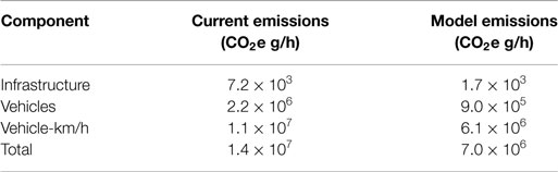
Table 3. Comparison of current and model green house gas emissions.

Our analysis shows that the optimization of the Barcelona transit network would not only lead to cost reductions, but would have a large effect on the potential level of GHG emissions. While system costs are reduced by 17%, the GHG emissions are reduced by 50%. The set of design parameters associated with this analysis comprise the cost-optimal point with regards to emissions. That is, costs are being minimized without any emission-based constraints. As decision makers become more concerned with specific emission standards in the future, additional constraints regarding emission levels may be implemented in the optimization. This will allow network designs to be based on the trade-offs between costs and GHG emissions. In the following section, we will discuss implications and suggestions for future work regarding these findings.

Conclusion

The findings presented in the previous section offer insights for transit agency decision makers. The optimization of a transit network—with the intention of making it a competitive alternative to the automobile—can lead to drastic reductions in both costs and emissions. The case study of Barcelona showed that applying this optimization process not only led to cost and emission reductions but maintained the level of service provided to the users. The approach taken in the examination of Barcelona can be applied to many cities in the world that utilize a transit system.

The constraints that were in place for the Barcelona case study would be paralleled by similar design restrictions in other cities, and could easily be accounted for in the optimization and analysis process. In Barcelona, as previously stated, there were design constraints set forth by the city regarding the minimum allowable headways and the maximum number of available corridors. Restrictions similar to these exist in other cities and must be taken into consideration when developing a model. Furthermore, once a model is created and decision variables are yielded, additional modifications must be considered to fit the geography and demand centers of the city, as was done by Estrada et al. (2011).

The reductions achieved in this case study did not have an effect on ridership. Since level of service was not altered, demand elasticity was not addressed in this paper. In future work, as models yield varying levels of service to users, demand elasticity should be considered. While we hypothesize that a correlation between GHG emissions reduction and transit network optimization exists, more city scenarios must be examined to further support this claim. To better understand the effect on GHG emission reductions, cities with different layouts, demand densities, and wage rates could be studied. The focus of this paper has been to address cost-optimal network design, which assumes that no costs are associated with GHG emission reductions. Griswold et al. (2013) incorporate emission constraints into their optimization and thereby are able to look at market value of GHG emissions. Future work may examine how current networks can move toward both cost-optimal designs as well as designs that take into account trade-offs between GHG emissions and total costs.

Author Contributions

Substantial contributions to the conception or design of the work; or the acquisition, analysis, or interpretation of data for the work: JG*, TS*, SM, AH, and JL. Drafting the work or revising it critically for important intellectual content: JG, TS, SM*, AH*, and JL. Final approval of the version to be published: JG, TS, SM*, AH, and JL*. Agreement to be accountable for all aspects of the work in ensuring that questions related to the accuracy or integrity of any part of the work are appropriately investigated and resolved: JG, TS, SM, AH, and JL. *Leading author who made crucial contributions to the corresponding criterion.

Conflict of Interest Statement

The authors declare that the research was conducted in the absence of any commercial or financial relationships that could be construed as a potential conflict of interest.

References

Byrne, B. F. (1975). Public transportation line positions and headways for minimum user and system cost in a radial case. Transp. Res. 9, 97–102. doi: 10.1016/0041-1647(75)90044-1

CrossRef Full Text | Google Scholar

Chester, M. V. (2008). Life-Cycle Environmental Inventory of Passenger Transportation Modes in the United States. Ph.D. dissertation, University of California, Berkeley, CA. Available at: http://repositories.cdlib.org/its/ds/UCB-ITS-DS-2008-1/

Google Scholar

Chester, M. V., and Horvath, A. (2009). Environmental assessment of passenger transportation should include infrastructure and supply chains. Environ. Res. Lett. 4, 024008. doi:10.1088/1748-9326/4/2/024008

CrossRef Full Text | Google Scholar

Daganzo, C. F. (2010). Structure of competitive transit networks. Transp. Res. Part B Methodol. 44, 434–446. doi:10.1016/j.trb.2009.11.001

CrossRef Full Text | Google Scholar

Environmental Protection Agency. (2014). Inventory of U.S. Greenhouse Gas Emissions and Sinks: 1990-2012 (EPA Publication No. 430-R-14-003). Washington, DC: U.S. Environmental Protection Agency.

Google Scholar

Estrada, M., Roca-Riu, M., Badia, H., Robusté, F., and Daganzo, C. F. (2011). Design and implementation of efficient transit networks: procedure, case study and validity test. Transp. Res. A Policy Pract. 45, 935–950. doi:10.1016/j.tra.2011.04.006

CrossRef Full Text | Google Scholar

Gallivan, F., and Grant, M. (2010). Current Practices in Greenhouse Gas Emissions Savings from Transit. TCRP Synthesis 84. Transportation Research Board. 85. doi:10.17226/14385

CrossRef Full Text | Google Scholar

Griswold, J. B. (2013). Tradeoffs between Costs and Greenhouse Gas Emissions in the Design of Urban Transit Systems. Ph.D. dissertation, University of California, Berkeley, CA. Available at: http://www.uctc.net/research/UCTC-DISS-2013-06.pdf

Google Scholar

Griswold, J. B., Madanat, S., and Horvath, A. (2013). Tradeoffs between costs and greenhouse gas emissions in the design of urban transit systems. Environ. Res. Lett. 8, 044046. doi:10.1088/1748-9326/8/4/044046

CrossRef Full Text | Google Scholar

Herndon, S. C., Shorter, J. H., Zahniser, M. S., Wormhoudt, J., Nelson, D. D., Demerjian, K. L., et al. (2005). Real-time measurements of SO2, H2CO, and CH4 emissions from in-use curbside passenger buses in New York City using a chase vehicle. Environ. Sci. Technol. 39, 7984–7990. doi:10.1021/es0482942

PubMed Abstract | CrossRef Full Text | Google Scholar

Holroyd, E. M. (1967). “The optimum bus service: a theoretical model for a large uniform urban area,” in Proceedings of the Third International Symposium on the Theory of Traffic Flow (New York: Elsevier).

Google Scholar

Kahn Ribeiro, S., Kobayashi, S., Beuthe, M., Gasca, J., Greene, D., Lee, D. S., et al. (2007). “Transport and its infrastructure,” in Climate Change 2007: Mitigation. Contribution of Working Group III to the Fourth Assessment Report of the Intergovernmental Panel on Climate Change, eds B. Metz, O. R. Davidson, P. R. Bosch, R. Dave and L. A. Meyer (Cambridge: Cambridge University Press).

Google Scholar

Newell, G. F. (1979). Some issues relating to the optimal design of bus routes. Transp. Sci. 13, 20–35. doi:10.1287/trsc.13.1.20

CrossRef Full Text | Google Scholar

Poudenx, P. (2008). The effect of transportation policies on energy consumption and greenhouse gas emission from urban passenger transportation. Transp. Res. Part A Policy Pract. 42, 901–909. doi:10.1016/j.tra.2008.01.013

CrossRef Full Text | Google Scholar

Puchalsky, C. (2005). Comparison of emissions from light rail transit and bus rapid transit. Transp. Res. Rec. 1927, 31–37. doi:10.3141/1927-04

CrossRef Full Text | Google Scholar

Appendix

A. Mathematical Program for Network Optimization

The following mathematical program was presented in Estrada et al. (2011) and is based on derivations performed by Daganzo (2010).

Most variables are defined within the paper; those which have not been previously presented are defined here.

The objective function is based on total system cost and is subject to several constraints: the spacing value must be greater than zero, the horizontal and vertical spacings, s_x and s_y, respectively, are integer multiples of the stop spacing s, the geometry proportions must be realistic, the headway must not be lower than a specified minimum headway, and the occupancy of vehicles, O_x and O_y (passengers), must not exceed capacity C (passengers), which is set to 150 for consistency with Estrada et al. (2011). The vehicle capacity should be re-adjusted if different vehicle types or transit modes are considered.

$\begin{array}{l}\hfill \text{min\hspace{0.17em}}{Z}_{\text{system}}=\left[{\mathrm{\pi }}_V\ast V+{\mathrm{\pi }}_M\ast M+{\mathrm{\pi }}_L\ast L\right]+\left[A+W+T+\left(\frac{\mathrm{\delta }}{v_w}\right)\ast e_T\right]\end{array}$

subject to s > 0; $s_x=p_{x}s;s_y=p_{y}s;p_x,p_y\text{integer};\frac{s_x}{D_x}\le {\mathrm{\alpha }}_x;\frac{s_y}{D_y}\le {\mathrm{\alpha }}_y;\text{H}\ge {\text{H}}_{\text{min}}$;

$O_x\le C;O_y\le C$

The length, L, of the infrastructure required is based on the geometry of the layout as a function of several decision variables.

$L=\frac{D_x{D}_y}{2s_x{s}_y}\left(s_x+s_y\right)\left(1+{\mathrm{\alpha }}_x{\mathrm{\alpha }}_y\right)+\frac{D_x{D}_y}{2s_x{s}_y}\left(s_x-s_y\right)\left({\mathrm{\alpha }}_y-{\mathrm{\alpha }}_x\right)$

The average vehicular distance traveled per hour of operation is a function of the geometric layout of the network as well as the service frequency.

$\begin{array}{l}\hfill V=\frac{2{\mathrm{\alpha }}_x{D}_x{D}_y}{s_{y}H}\left[1+\frac{D_x}{2D_y}\left(1-{\mathrm{\alpha }}_x\right)\right]+\frac{2{\mathrm{\alpha }}_y{D}_x{D}_y}{s_{x}H}\left[1+\frac{D_y}{2D_x}\left(1-{\mathrm{\alpha }}_y\right)\right]\end{array}$

The occupancies of the vehicles are determined by the catchment area of bus routes, service frequency, and the trip generation rate during rush periods, Λ (passengers/hr).

$\begin{array}{l}{O}_x=\text{max}\left(\frac{\Lambda s_{x}H\left(1+{\mathrm{\alpha }}_y\right)\left(1-{\mathrm{\alpha }}_x\right)}{4{\mathrm{\alpha }}_y{D}_y};\frac{\Lambda H{\left(1-{\mathrm{\alpha }}_y\right)}^2{\left(1+{\mathrm{\alpha }}_x\right)}^2}{32}\right.\left.+\frac{\Lambda s_{x}H(4-{(1+{\text{α}}_x)}^2{(1-{\text{α}}_y)}^2-2{\text{α}}_x^2{\text{α}}_y^2}{(8{\text{α}}_y{D}_y)}\right)\hfill \\ O_y=\text{max}\left(\frac{\Lambda s_{y}H\left(1+{\mathrm{\alpha }}_x\right)\left(1-{\mathrm{\alpha }}_y\right)}{\left(4{\mathrm{\alpha }}_x{D}_x\right)};\frac{\Lambda H{\left(1-{\mathrm{\alpha }}_x\right)}^2{\left(1+{\mathrm{\alpha }}_y\right)}^2}{32}\right.\left.+\frac{\Lambda s_{y}H(4-{(1+{\text{α}}_y)}^2{(1-{\text{α}}_x)}^2-2{\text{α}}_x^2{\text{α}}_y^2}{8{\text{α}}_x{D}_x}\right)\hfill \end{array}$

The number of vehicles required in the fleet is a function of the vehicle-km/h traveled V divided by the commercial speed of the bus v_c (km/hr).

$\begin{array}{l}\hfill M=\frac{V}{v_c}\end{array}$

The following formulas address the values concerned with user costs. That is, the various components that contribute to the time users spend in the system. The access time A is a function of the distance an average user must walk and an average walking speed v_w.

$A=\frac{\frac{s_x+s_y}{4}+\frac{s}{2}}{v_w}$

The average waiting time that users experience W is a function of the service frequency, the network layout, and the probabilities of users experiencing one or two transfers, P₁ and P₂ respectively. The occupancy of vehicles is constrained below capacity so that users can take the first bus that arrives.

$\begin{array}{l}W=\left[\frac{H}{6{\mathrm{\alpha }}_x}\left(1-{\mathrm{\alpha }}_x^3\right)\frac{\left(1-{\mathrm{\alpha }}_y\right)}{\left(1-{\mathrm{\alpha }}_x\right)}+\frac{H}{6{\mathrm{\alpha }}_y}\left(1-{\mathrm{\alpha }}_y^3\right)\frac{\left(1-{\mathrm{\alpha }}_x\right)}{\left(1-{\mathrm{\alpha }}_y\right)}\right.\left.+{\mathrm{\alpha }}_x{\mathrm{\alpha }}_y\frac{H}{2}\right]\left(1+P_1\right)+\frac{H}{2}{P}_2\hfill \\ P_1=\frac{s_y}{2D_x}\left(-{\mathrm{\alpha }}_y+{\mathrm{\alpha }}_y^2-3{\mathrm{\alpha }}_x{\mathrm{\alpha }}_y+{\mathrm{\alpha }}_x{\mathrm{\alpha }}_y^2\right)+\frac{s_x}{2D_y}\left(-{\mathrm{\alpha }}_x+{\mathrm{\alpha }}_x^2-3{\mathrm{\alpha }}_x{\mathrm{\alpha }}_y+{\mathrm{\alpha }}_y{\mathrm{\alpha }}_x^2\right)\\ +\frac{1}{2}\left(1-{\mathrm{\alpha }}_y^2-{\mathrm{\alpha }}_x^2+4{\mathrm{\alpha }}_x{\mathrm{\alpha }}_y-{\mathrm{\alpha }}_x^2{\mathrm{\alpha }}_y^2\right)+\frac{s_x{s}_y{\mathrm{\alpha }}_x{\mathrm{\alpha }}_y}{D_x{D}_y}\\ P_2=\frac{1}{2}\left(1+{\mathrm{\alpha }}_y^2+{\mathrm{\alpha }}_x^2-4{\mathrm{\alpha }}_x{\mathrm{\alpha }}_y+{\mathrm{\alpha }}_x^2{\mathrm{\alpha }}_y^2\right)-\frac{s_y}{2D_x}{\left(1-{\mathrm{\alpha }}_y\right)}^2\left(1+{\mathrm{\alpha }}_x\right)-\frac{s_x}{2D_y}{\left(1-{\mathrm{\alpha }}_x\right)}^2\left(1+{\mathrm{\alpha }}_y\right)\hfill \end{array}$

The expected number of transfers e_T is determined by using these probabilities:

$e_T=P_1+2P_2$

Finally, the in-vehicle travel time T is determined by relating the in-vehicle travel distance E with the commercial speed of the buses v_c. The formula for the distance is given below.

$\begin{array}{l}E=\left(\frac{{\mathrm{\alpha }}_y^2{D}_y^2+{\mathrm{\alpha }}_x^2{D}_y^2+4{\mathrm{\alpha }}_x{\mathrm{\alpha }}_y{D}_x{D}_y}{4\left({\mathrm{\alpha }}_x{D}_x+{\mathrm{\alpha }}_y{D}_y\right)}\right.\left.+\frac{{\mathrm{\alpha }}_x{D}_x+{\mathrm{\alpha }}_y{D}_y}{12{\mathrm{\alpha }}_x{\mathrm{\alpha }}_y{D}_x{D}_y}\left(1-\frac{{\mathrm{\alpha }}_x{\mathrm{\alpha }}_y}{2}\right)\right)\left(1-{\mathrm{\alpha }}_x^2{\mathrm{\alpha }}_y^2\right)\hfill \\ +\frac{1}{3}\left({\mathrm{\alpha }}_x{D}_x+{\mathrm{\alpha }}_y{D}_y\right)\left({\mathrm{\alpha }}_x^2{\mathrm{\alpha }}_y^2\right)+\frac{1}{4}\left(D_x\left(2-3{\mathrm{\alpha }}_x+{\mathrm{\alpha }}_x^3\right)\right.\left.+D_y\left(2-3{\mathrm{\alpha }}_y+{\mathrm{\alpha }}_y^3\right)\right)\end{array}$

B. Cost Calculations

TABLE B1

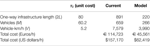
Table B1. Agency costs.

TABLE B2

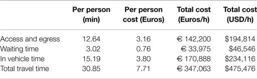
Table B2. User costs, model predictions.

TABLE B3

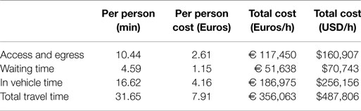
Table B3. User costs, current system.

TABLE B4

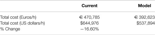
Table B4. Cost overview.