On the Performance of Online Parameter Estimation Algorithms in Systems with Various Identifiability Properties

1. Introduction

In the last decade, acknowledgment of the current critical state of our infrastructure [highlighted for instance by the 2013 Report Card for Americas Infrastructure giving a D+ grade to Americas infrastructure, ASCE (2016)], along with a growing interest in sustainable and resilient infrastructure systems, has led researchers to focus efforts on condition monitoring for better management of civil structures. Many complementary methods can be used for the purpose of damage detection and monitoring of structures; these include non-destructive evaluation, visual inspection, or vibration-based methods. The latter are based on the idea that introduction of damage will modify the response behavior of the structure; thus, by measuring the structure’s response, one will be able to detect changes that may be indicators of damage.

This paper focuses on model-based methods, which make use of a known physical model of the structure, whose parameters and part of its structure are learnt using measurements from the system and system identification algorithms. By comparing the updated model of the structure with its known/assumed healthy model, one can detect changes in the structure and correlate them to potential damage. In this way, one is able to identify, localize, and possibly evaluate the cause and extent of damage [hierarchy of damage detection, Rytter (1993)]. Furthermore, very importantly for structural health monitoring purposes, this kind of method provides the user with a model of the structure in its damaged state, which can be used for prognosis purposes (i.e., to determine the remaining life of the structure of interest).

More specifically, we look at dynamical systems that follow a known process equation of the form ${\dot{x}}^{\mathit{dyn}}\left(t\right)=\tilde{f}\left(x^{\mathit{dyn}}\left(t\right),\mathrm{\theta },e\left(t\right)\right)$, where x^dyn(t) represent the dynamic states (displacements, velocities…), θ the vector of static parameters (stiffness, damping…), which characterize the system and e(t) a known forcing function. For damage assessment, one wants to study the behavior of the dynamic states x^dyn(t) (e.g., for fatigue monitoring) and/or learn the static parameters θ, since a change in a parameter can indicate presence of damage at this location. Measurements, such as accelerations and strains, are then performed on the structure, and system identification tools are used to estimate the states/parameters from these series of measurements y. Due to inherent uncertainties in real-life applications (modeling and measurement errors for instance), statistical models must be used, i.e., the measurements are related to the states and parameters through an equation of the form

$y=h\left(x^{\mathit{dyn}},\mathrm{\theta }\right)+\underset{\text{errors}}{\underbrace{\mathrm{\eta }}}$ (1)

Looking solely at parameter estimation, two main approaches compete (see Figure 1). In the frequentist approach, parameters are assumed to be fixed but unknown, and an estimate $\widehat{\theta }$ can be learnt through statistical minimization of the error between the measurements y and the deterministic model outputs h(x^dyn, θ) (e.g., least-squares or maximum-likelihood estimators). In contrast, Bayesian techniques consider parameters as random variables (RVs) and make use of the measurements to update some prior knowledge (prior probability density function pdf, or moments) and thus yield the posterior pdf (or moments). A crucial advantage of the Bayesian framework lies in the fact that it is able to tackle ill-conditioned problems where some or all parameters cannot be uniquely identified based on available measurements (Muto and Beck, 2008), which is a major topic of this paper. For identification of parameters, Bayes’ theorem can be written as

$\stackrel{\text{posterior}}{\overbrace{p\left(\mathrm{\theta }|y\right)}}=\frac{\stackrel{\text{likelihood}}{\overbrace{p\left(y|\mathrm{\theta }\right)}}\stackrel{\text{prior}}{\overbrace{p\left(\mathrm{\theta }\right)}}}{p\left(y\right)}=\frac{p\left(y|\mathrm{\theta }\right)p\left(\mathrm{\theta }\right)}{\int p\left(y|\mathrm{\theta }\right)p\left(\mathrm{\theta }\right)d\mathrm{\theta }}$ (2)

FIGURE 1

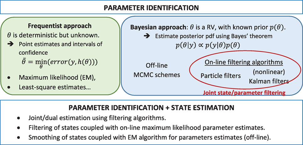
Figure 1. Parameter learning and state estimation.

Lately, research efforts have been mostly directed toward Markov Chain Monte Carlo (MCMC) techniques, which make use of the importance sampling principle (Figure 2) to efficiently explore the parameter space [see, e.g., Smith (2014) for an introduction to freqentist/Bayesian approaches and MCMC techniques]. MCMC techniques build Markov chains whose stationary distribution is the posterior pdf, thus sampling from the chain yields an estimate of the posterior pdf. MCMC techniques are offline methods; they necessitate running the entire forward problem with different values of the parameter vector θ, each of them being selected based on the previous value. Furthermore, they are very computationally expensive for medium to large dimensional problems. Ongoing research focuses on deriving novel algorithms that more efficiently explore the parameter space [Data Annealing principle, see Green (2015), sampling from a sequence of intermediate distributions which converge to the posterior, see, e.g., Beck and Au (2002), Ching and Chen (2007), and Beck and Zuev (2013)].

FIGURE 2

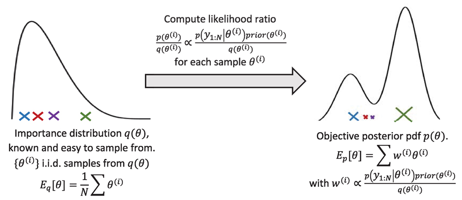
Figure 2. Principle of importance sampling, used in MCMC and particle filter schemes. If q(θ) = prior(θ), the weights are then simply proportional to the likelihood p(y_1:N|θ) (bootstrap PF).

Both approaches have been shown to be applicable for structural health monitoring purposes, using experimental data. Some recent work include the study by Jang and Smyth (2017), in which a full-scale FEM model of a bridge is updated to match modal properties coming from real measured data: updating parameters are chosen using a sensitivity-based algorithm, then the optimized parameters are computed through minimization of an error function on the modal properties (frequentist approach); in Jang (2016), the authors also use Bayesian inference (MCMC) to learn the parameters, based on the same measured data. In Dubbs and Moon (2015), several multiple model identification methods (i.e., multiple parameter sets, contrary to frequentist approaches that yield one single value for θ) are compared using experimental data, and it is concluded that the Bayesian approach is the most efficient and most precise for the problem considered. In Pasquier and Smith (2016), parameter identification, using either MCMC or other sampling techniques, is integrated into a global framework, which performs iterations of modeling/FE model falsification in order to sequentially acquire knowledge about the structure; the performance of this approach is assessed on measured data from a bridge.

This paper focuses more specifically on online identification, which can also be performed in the Bayesian setting, using sequential Bayesian filtering algorithms such as the widely known Kalman filter for state estimation in linear systems. At each time step k, these sequential algorithms make use of the new available measurement y_k to update the posterior pdf, possibly in real time. Online filtering enables real-time monitoring of both states and parameters, and thus provides quick insight into the behavior of the system for fast decision-making procedures. This paper first reviews the basics of online Bayesian filtering [see, e.g., Särkkä (2013) for a thorough exploration of filtering and smoothing], along with the main algorithms used in the literature. Then, the performance of these algorithms in identifying static parameters of structural systems is studied, and it is shown that the behavior of the algorithms largely depends on the identifiability characteristics of the system.

2. Bayesian Filtering for Online Parameter Identification

2.1. Motivation and Challenges

In order to use online Bayesian inference techniques, one must cast the system of interest in the state-space framework and discretize it in time to yield a process equation of the form $x_{k+1}^{\mathit{dyn}}=f\left(x_k^{\mathit{dyn}},\mathrm{\theta },e_k\right)$, where again x^dyn represent the dynamic states, θ the vector of static parameters and e_k a known forcing function. We then consider the generic non-linear dynamic system in state-space form defined by the following system equations:

$x_k^{\mathit{dyn}}=f\left(x_{k-1}^{\mathit{dyn}},\mathrm{\theta },e_{k-1}\right)+v_{k-1}\left(\text{propagation equation}\right)$ (3a)

$y_k=h\left(x_k^{\mathit{dyn}},\mathrm{\theta }\right)+{\mathrm{\eta }}_k\left(\text{observation equation}\right)$ (3b)

where f(⋅) and h(⋅) are usually non-linear functions. v_k and η_k are the system noise and observation noise, such that

$\text{E}\left[v_k\right]=0,\text{E}\left[{\mathrm{\eta }}_k\right]=0$ (4a)

$\text{E}\left[v_j{v}_k^T\right]=Q{\mathrm{\delta }}_{\mathit{jk}},\text{E}\left[{\mathrm{\eta }}_j{\mathrm{\eta }}_k^T\right]=R{\mathrm{\delta }}_{\mathit{jk}},\text{E}\left[v_{k,k-1}{\mathrm{\eta }}_k^T\right]=0$ (4b)

i.e., the process and measurement noise are white, zero-mean and uncorrelated to each other (E[⋅] denotes the mathematical expectation). In this paper, we will consider only additive Gaussian noise terms, as shown in equation (3). Extension of filtering algorithms such as the unscented Kalman filter (UKF) and the generic particle filter (PF), presented in the next section, to non-additive noise could be achieved by adding the noise terms in the state vector and considering f and h as functions of both the states and the noise. In this paper however, we will make use of the so-called Rao-Blackwellisation principle (see section 2.2.1) to increase efficiency of the particle filter, which can be solely used in the presence of additive Gaussian noise. Also, we will assume that the covariance terms Q and R are known; however, the parameters of these noise terms could also be learnt using Bayesian inference (see for instance, Kontoroupi and Smyth (2016) for the UKF and Özkan et al. (2013) for the PF, for learning of additive Gaussian noise terms).

2.1.1. Parameter Estimation through Joint Filtering

For online estimation of the full posterior pdf (both states and parameters), several methods can be used. A very common approach is to perform joint state/parameter filtering, that is, the state vector is augmented with the static parameters which are assigned the propagation equation θ_k = θ_k−1. The state vector then becomes $x_k=\left\{\begin{array}{c}\hfill x_k^{\mathit{dyn}}\hfill \\ \hfill \mathrm{\theta }\hfill \end{array}\right\}$, and ateach time step, the full posterior pdf $p\left(x_k^{\mathit{dyn}},\mathrm{\theta }|y_{1:k}\right)=p\left(x_k|y_{1:k}\right)$ is inferred. This method is used in the remainder of the paper.

Another approach commonly used consists of separating estimation of the dynamic states and identification of the parameters. In Wan and Van Der Merwe (2000), an online dual approach is presented, where two filtering algorithms (UKFs) are run in parallel, one for estimation of the states, the other for estimation of the parameters, and both make use of the current estimates from the concurrent filter to propagate to the next time step. Other dual approaches can also be derived by combining a state filtering scheme with any parameter learning algorithm. For instance, in the study by Poyiadjis et al. (2006), online estimation of both states and parameters is performed by combining a particle filter for state estimation and an online maximum likelihood estimation procedure for the parameters, while in the study by Lindsten (2013), an offline procedure is presented, combining a particle smoother for the states with an expectation–maximization (EM) algorithm for the parameters.

2.1.2. A Challenge to Parameter Estimation: Parameter Identifiability

Parameter identification in real-life applications is a very challenging task since the structure and excitations to which it is subjected might not be fully known, and measurements from the structure will likely be sparse and noisy. In this paper, we assume that the system equations are known (i.e., the same equations of motion are used to simulate data and to run the inverse problem¹) and that we have access to noisy measurements of the excitation. These assumptions could be relaxed by (1) learning both the parameters of the model and part of its structure through Bayesian model selection algorithms for instance (see, e.g., Kontoroupi and Smyth (2017) for an online version); and (2) follow the method presented in the study by Olivier and Smyth (under review)² to take into account unmeasured stationary excitations in filtering algorithms, in case no direct measurement of the excitation at each DOF is available.

The fact that one has access to a limited number of measurements at specific locations on the structure raises the questions of state observability and parameter identifiability. Looking solely at identification of static parameters θ, the question of identifiability can be stated simply as whether running the inverse problem using the available measurements yield an infinite number of solutions for the vector θ (unidentifiable), a finite number of solutions (local identifiability), or a unique solution (global identifiability). Knowing the system equations, identifiability can be tested using various algorithms, see for instance, Chatzis et al. (2015) for a discussion on the subject for non-linear systems. It has to be noted, however, that those tests assume that (1) the excitation is exactly known and (2) the system is noise free. Since in real-life systems are always noisy, one will use probabilistic methods when identifying parameters, even though the noise-free system has a unique parameter solution. For non-linear systems, introduction of noise in the system can actually render a parameter “unidentifiable,” even though it is identifiable for the noise-free system (see example in section 3.1).

Identifiability of a system is a property of the system itself (equations of motion and available measurements) and does not depend on the method used to identify the parameters (frequentist vs. Bayesian, online vs. offline). However, since identification methods are based on learning from the measurements, the identifiability properties of the system will have a direct impact on the posterior pdfs p(θ|y_1:N), and thus on the choice of filtering algorithm used to perform the inverse problem, as will be explained through several examples in section 3. For systems that are globally identifiable (there exists a unique solution to the inverse problem), posterior pdfs would be expected to be unimodal, with relatively small variance, indicating that having access to measurements yields improved knowledge of the parameters. For unidentifiable parameters, one would expect the posterior and the prior pdfs to be relatively close to each other (no learning is possible using the measurements). For locally identifiable parameters (i.e., several parameters would lead to the same measured system response), one would expect multimodal posterior pdfs.

In the study by Vakilzadeh et al. (2017), an ABC technique (Approximate Bayesian Computation, an offline parameter estimation method that does not require explicit knowledge of the likelihood function, contrary to MCMC schemes) is used on several problems which exhibit various identifiability properties, and one can observe that this offline technique is indeed able to capture non-Gaussian, possibly multimodal posterior pdfs. In this paper, we study the behavior of online algorithms to parameter identification in systems that also show different identifiability characteristics, some of them adapted from the study by Vakilzadeh et al. (2017). The idea is to provide an insight into the kind of behavior to expect from fast online parameter learning algorithms, depending on the problem at hand, thus guiding the choice of algorithm for future users. We start by reviewing the two main algorithms used in this paper: the particle filter and the unscented Kalman filter.

2.2. Review of Online Bayesian Filtering Algorithms

The reader is referred to the study by Särkkä (2013) for a more in-depth review of the Bayesian filtering formulation. Briefly, sequential filtering techniques use the Markovian properties of the system (x_k given x_k−1, and y_k given x_k, are independent of other past states and past observations) to infer at each time step k the posterior pdf of the states knowing all the past observations, i.e., p(x_k|y_1:k). The Bayesian filtering equations are decomposed into two steps:

• Propagation step (Chapman–Kolmogorov equation), learn the prior pdf at time step k:

$p\left(x_k|y_{1:k-1}\right)=\int p\left(x_k|x_{k-1}\right)p\left(x_{k-1}|y_{1:k-1}\right){\mathit{dx}}_{k-1}$ (5a)

• Update step, make use of the new measurement y_k and Bayes’ theorem to derive the posterior distribution at time step k:

$p\left(x_k|y_{1:k}\right)=\frac{p\left(y_k|x_k\right)p\left(x_k|y_{1:k-1}\right)}{p\left(y_k|y_{1:k-1}\right)}$ (5b)

2.2.1. Particle Filtering

Particle filtering schemes use Monte Carlo approximations of the posterior density, i.e., it is represented by a finite number of weighted samples (particles) as

$p\left(x_k|y_{1:k}\right)\approx {\displaystyle \sum _{i=1}^{n_p}}{w}_k^{\left(i\right)}\mathrm{\delta }\left(x_k-x_k^{\left(i\right)}\right)$ (6)

where ${\left\{x_k^{\left(i\right)},w_k^{\left(i\right)}\right\}}_{i=1:n_p}$ are the sampled particles and their associated weights, respectively (see further details and Figure 3), n_p the number of particles used for the approximation, and δ(⋅) is the delta dirac function. Expectations of functions φ of x_k (moments for instance) are computed by sample averages:

$E\left[\mathrm{\phi }\left(x_k\right)|y_{1:k}\right]\approx {\displaystyle \sum _{i=1}^{n_p}}{w}_k^{\left(i\right)}\mathrm{\phi }\left(x_k^{\left(i\right)}\right)$ (7)

FIGURE 3

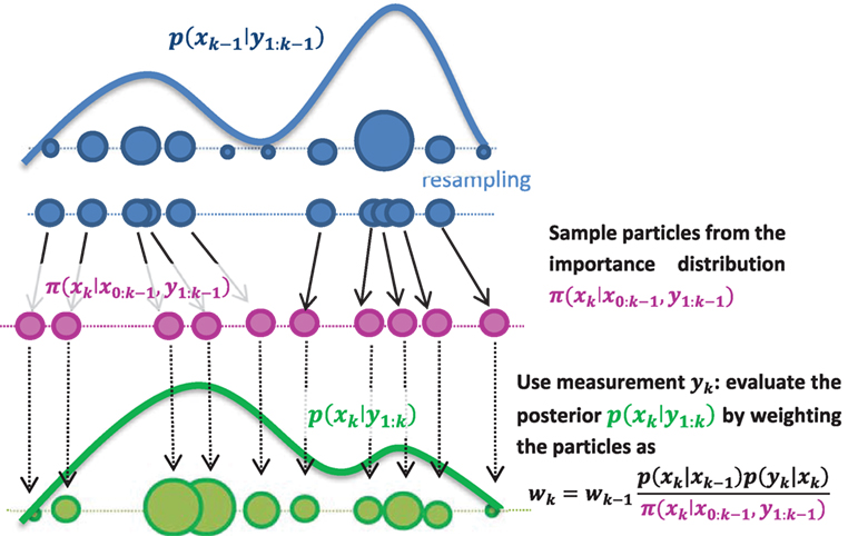
Figure 3. One time step of the particle filter: importance sampling is used, i.e., sample particles from an importance density π(x_k|x_0:k−1, y_1:k) then weight them proportionally to their likelihood. In the so-called bootstrap particle filter, the simplest version of the PF, one simply samples particles from the transition density $p\left(x_k|x_{k-1}^{\left(i\right)}\right)$, thus obtaining a particle approximation of the prior p(x_k|y_1:k−1). Then, the weighting equation simplifies to $w_k^{\left(i\right)}=w_{k-1}^{\left(i\right)}p\left(y_k|x_k^{\left(i\right)}\right)$.

Only a brief review of the theory of particle filtering is provided in this paper. For more details on the theory of particle filtering, one can refer, for example, to Cappé et al. (2007), Doucet and Johansen (2011), and Särkkä (2013). The particle filter is a sequential importance sampling (SIS) algorithm, which can be summarized as in Figure 3: at each time step k, one samples particles from an importance (sometimes called proposal) distribution, then weights the particles proportionally to their likelihood. The weighted set of particles provides a particle approximation [equation (6)] of the posterior pdf p(x_k|y_1:k). However, as this is done sequentially over a large number of steps, one usually ends up with a set of particles among which only a few have significant weights (impoverishment). The worst-case scenario is when only one particle has weight one: this is called collapse of the PF (the posterior pdf becomes a single dirac function). To overcome this issue, one adds a resampling scheme to the algorithm, the goal being to duplicate particles with high weight while getting rid of particles with low weights, thus focusing on regions of high likelihood.

Convergence of the bootstrap particle filter is studied for instance in the study by Crisan and Doucet (2002), where it is shown that, under some assumptions regarding the resampling step, the bootstrap particle filter converges to the true posterior pdf when the number of particles goes to infinity. Several authors have shown that in practice the number of particles should increase exponentially with the dimension of the system to avoid collapse (see for instance, Bengtsson et al. (2008) and Rebeschini and van Handel (2015) for a more detailed discussion on PF vs. curse of dimensionality).

The sample impoverishment issue is exacerbated in the particle filter when static parameters are added to the state vector. This is a major drawback of the PF in the context of damage detection since one wants to monitor the behavior of the static parameters of the system. Thus, we will use in our numerical experiments, whenever possible, the so-called marginalized particle filter for mixed linear/non-linear systems (derived in the study by Schön et al. (2005), simply called RBPF in the remainder of this paper), which makes use of the principle of Rao-Blackwellisation and was proved to behave efficiently for structural systems (see for instance, Olivier and Smyth (2017a)). The main idea behind Rao-Blackwellisation in the particle filtering context (Doucet et al., 2000) is to decompose the state vector into $x_k={\left[\begin{array}{cc}\hfill u_k^T\hfill & \hfill z_k^T\hfill \end{array}\right]}^T$ and write the system as

$x_k=F\left(u_{k-1}\right)z_{k-1}+f\left(u_{k-1}\right)+v_{k-1}$ (8a)

$y_k=H\left(u_k\right)z_k+h\left(u_k\right)+{\mathrm{\eta }}_k$ (8b)

Conditioned on u_k−1 and u_k, the posterior of z can be exactly inferred using the Kalman filter equations (assuming Gaussian prior for z and Gaussian noise). The marginal posterior pdf can be written as

$p\left(u_k,z_k|y_{1:k}\right)={\displaystyle \sum _{i=1}^{n_p}}{w}_k^{\left(i\right)}\mathcal{N}\left(z_k;z_{k|k}^{\left(i\right)},P_{k|k}^{\left(i\right)}\right)\mathrm{\delta }\left(u_k-u_k^{\left(i\right)}\right)$ (9)

where $\mathcal{N}\left(a;b,C\right)$ denotes the Gaussian distribution with mean b and covariance C evaluated at point a. The posterior pdf is now represented as a mixture of n_p Gaussians in the dimensions of partition z_k, and it still converges to the true posterior pdf as n_p → ∞. It is important to notice here that no Gaussian assumption is used for the posterior pdf, contrary to UKF algorithms described in the next section. Instead, some properties of the system equations (conditional linearities) are used to perform some calculations analytically, thus reducing the sampling variance of the estimates.

Performing some calculations analytically using this concept helps avoid the degeneracy issue, especially if z is composed of the static parameters, which will be the case for many structural systems. Figure 4 shows the behavior of the generic PF vs. a Rao-Blackwellised PF on the convergence of the stiffness parameters of a 3-DOF system with one high non-linearity at the base (results presented in the study by Olivier and Smyth (2017a)). With 500 particles, the generic PF collapses while the Rao-Blackwellised PF converges to the true values of the stiffness parameters.

FIGURE 4

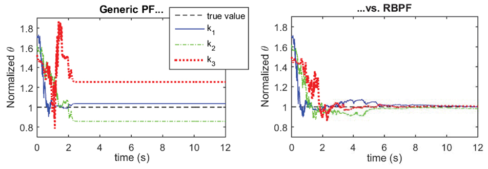
Figure 4. Performance comparison of generic PF (left plot, collapse of the PF which yields incorrect estimates) vs. Rao-Blackwellised PF (right plot, improved performance) on identification of stiffness parameters of a 3-DOF system. For both algorithms, n_p = 500 particles are used for the estimation.

2.2.2. Non-Linear Kalman Filtering Schemes

In non-linear Kalman filtering, two approximations are used in order to simplify the filtering equations. First, recall that in the update step, one makes use of Bayes’ theorem to condition upon the new measurement y_k. If a Gaussian assumption is used for the pdfs p(x_k, y_k|y_1:k−1) and p(x_k|y_1:k), this update step can be written in closed form using properties of the Gaussian distribution, leading to the well-known Kalman filter measurement update equations:

$\text{E}\left[x_k|y_{1:k}\right]=x_{k|k-1}+K_k\left(y_k-y_{k|k-1}\right)$ (10a)

$\mathit{Cov}\left(x_k|y_{1:k}\right)=P_{k|k-1}-K_k{S}_k{K}_k^T$ (10b)

where

$x_{k|k-1}=\text{E}\left[x_k|y_{1:k-1}\right],P_{k|k-1}=\mathit{Cov}\left(x_k|y_{1:k-1}\right),$ (11a)

$y_{k|k-1}=\text{E}\left[y_k|y_{1:k-1}\right],S_k=\mathit{Cov}\left(y_k|y_{1:k-1}\right),$ (11b)

${\mathrm{\Psi }}_k=\mathit{Cov}\left(x_k|y_{1:k-1},y_k|y_{1:k-1}\right),$ (11c)

$K_k={\mathrm{\Psi }}_k{S}_k^{-1}\left(\text{Kalman gain}\right)$ (11d)

where Cov(X) denotes the covariance of a RV X, and Cov(X, Y) denotes the cross-covariance between jointly distributed RVs X and Y.

In the Gaussian linear case (where both f and h are linear, and the noise terms are Gaussian), the Gaussian assumption is exact and the Kalman filter equations yield the true posterior distributions in closed form. However in general, the propagation and observation equations f and h are not linear; thus, the pdfs p(x_k, y_k|y_1:k−1) and p(x_k|y_1:k) are not truly Gaussian and cannot be computed in closed form. The second approximation made in non-linear Kalman filtering is then to estimate the first and second order moments of those pdfs and build a Gaussian approximation using those moments. Two main methods are being used for this purpose:

• linearization using Taylor series expansion (yields the extended Kalman filter EKF),

• the unscented transform (yields the unscented Kalman filter UKF, see, e.g., Wan and Van Der Merwe (2000) and Julier and Uhlmann (2004)).

The unscented transform (UT, see, e.g., Julier and Uhlmann (2004) for a thorough review of the UT and UKF) aims at computing the moments of an output RV Z = g(X) (also written $X\stackrel{g}{\to }Z$), where g is a non-linear function, when the moments of the input RV X are known. It is used twice at each time step of the UKF:

$x_{k-1}\mathrm{|}{y}_{1:k-1}\stackrel{f}{\to }{x}_k\mathrm{|}{y}_{1:k-1}$

$x_k\mathrm{|}{y}_{1:k-1}\stackrel{h}{\to }{y}_k\mathrm{|}{y}_{1:k-1}$

The UT consists of evaluating the function g at certain points ${\mathcal{X}}^{\left(i\right)}$ in the X space, called sigma points, chosen deterministically to match the moments of the input RV X. Moments of the output Z are then computed by weighted averages over the transformed sigma points ${\mathcal{Ƶ}}^{\left(i\right)}=g\left({\mathcal{X}}^{\left(i\right)}\right)$. The accuracy of the UT depends on two properties:

• the level of non-linearity of the function g, and

• how many moments of the input RV X are matched by the sigma point set.

To understand this, one may consider the second-order approximations of the mean and covariance of Z = g(X) (in the univariate case, following for instance, Ang and Tang (2007)):

$\text{E}\left[Z\right]\simeq g\left({\mathrm{\mu }}_X\right)+\frac{1}{2}{\mathrm{\sigma }}_X^2\frac{d^{2}g}{{\mathit{dX}}^2}$ (12a)

$\mathit{Var}\left(Z\right)\simeq {\mathrm{\sigma }}_X^2{\left(\frac{\mathit{dg}}{\mathit{dX}}\right)}^2-\frac{1}{4}{\mathrm{\sigma }}_X^2{\left(\frac{d^{2}g}{{\mathit{dX}}^2}\right)}^2+\text{E}\left[{\left(X-{\mathrm{\mu }}_X\right)}^3\right]\frac{\mathit{dg}}{\mathit{dX}}\frac{d^{2}g}{{\mathit{dX}}^2}+\frac{1}{4}\text{E}\left[{\left(X-{\mathrm{\mu }}_X\right)}^4\right]{\left(\frac{d^{2}g}{{\mathit{dX}}^2}\right)}^2$ (12b)

where μ_X and ${\mathrm{\sigma }}_X^2$ are the known mean and variance of the input RV X, E[(X − μ_X)³], and E[(X − μ_X)⁴] its central third- and fourth-order moments. These are second order approximations in the sense that they keep only terms that contain up to the second-order derivatives of g and are thus exact for quadratic functions. To obtain second-order accuracy on computation of the mean E[Z], only knowledge of the first two moments of X is needed, however to obtain the same order of accuracy in computing the variance Var(Z) knowledge of higher order (3rd and 4th) moments of the input RV X is required.

Returning to the UT, the most widely used sigma point set in the UKF context is the symmetric (possibly scaled) set, which captures up to the second-order moment of the input RV X. It then achieves second-order accuracy in estimating the mean E[Z] = E[g(X)] but only first-order accuracy on its covariance estimate Cov(Z) = Cov(g(X)). Derivations of various sigma point sets can be found for instance in the studies by Julier and Uhlmann (1997, 2002) and Julier (1998, 2002), some of which are plotted in Figure 5. A more detailed discussion and examples of the order of accuracy of the UKF can also be found in the authors’ previous paper (Olivier and Smyth, 2017b). The UKF with symmetric sigma point set has been shown to behave very well for parameter identification for highly non-linear systems, as long as the noise terms are Gaussian and the parameters are identifiable. It does not require computations of Jacobians as in the EKF. Furthermore, for this symmetric sigma point, set the number of sigma points, and thus, the overall computational time of the algorithm grows only linearly with the dimension of the state vector, independent of the fact that it may contain static parameters (contrary to the particle filter, as explained in the previous section). Thus, the UKF usually achieves a good trade-off between accuracy and computational time and is very attractive for real-time monitoring purposes.

FIGURE 5

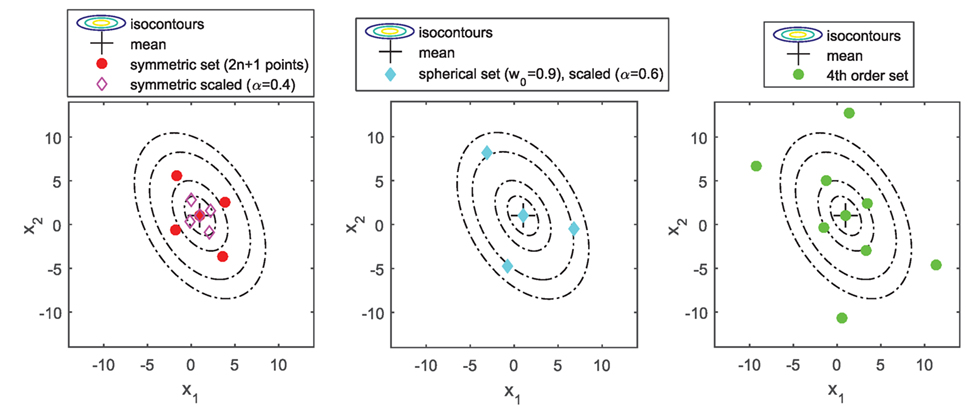
Figure 5. Various sigma point sets for use in the unscented transform.

In the following, we somewhat expand the discussion started in the study by Olivier and Smyth (2017b) to more complex problems that show different identifiability characteristics, and we study the performance of both the PF and UKF on these new problems of interest.

3. Performance of Algorithms for Systems with Different Identifiability Properties

3.1. Globally Identifiable Duffing Oscillator

The equation of motion for a Duffing oscillator, with known mass m = 1, subjected to a known ground acceleration a_g, is

$\ddot{\xi }\left(t\right)+c\dot{\xi }\left(t\right)+k_{\mathit{lin}}\mathrm{\xi }\left(t\right)+\mathrm{\beta \xi }{\left(t\right)}^3=-a_g\left(t\right)$ (13)

where ξ(t) represents the relative displacement of the mass, and c, k_lin, and β the damping, linear, and non-linear stiffness parameters, respectively. Global identifiability of this system, when measuring either displacement or velocity, can be assessed using for instance the identifiability software DAISY, presented in Bellu et al. (2007); meaning that the parameter vector $\mathrm{\theta }={\left[k_{\mathit{lin}}c\mathrm{\beta }\right]}^T$ can be theoretically identified in the absence of noise. If acceleration is measured, one can obtain an expression of the displacement through integration, with the condition that initial conditions are known; thus, global identifiability results also apply when measuring acceleration.

In real-life applications however, measurements will always incorporate some noise, which renders identification of some parameters much harder to perform. In the case of a Duffing oscillator, even though theoretically the non-linearity is excited as soon as |ξ| > 0, the presence of noise could render it impossible to detect unless it is excited at a high enough level. To incorporate noise in the simulated data, 10% root-mean-square (RMS) Gaussian noise is added to both acceleration time series ($\ddot{\xi }$ and a_g) before using them for parameter identification. Also, when performing real-time monitoring of a structure, it may not be reasonable to assume that initial conditions are known exactly. Thus, algorithms are initialized with a Gaussian prior on the states ${\left[{\mathrm{\xi }}^T{\dot{\xi }}^T\right]}^T$ with a non-zero variance (standard deviation is chosen as 20% RMS noise of the corresponding state signal).

Performance of both the UKF and the RBPF are compared using this simple problem. Also, the influence of the prior is studied by running simulations with three different priors for the unknown parameters: priors 1 and 2 are Gaussian, with different mean and covariance. Prior 3 is similar to prior 1 (Gaussian) for parameters k_lin,c, but it is a mixture of 3 Gaussians for the non-linear stiffness parameter β, which is harder to identify. In this way, this prior is more uniform over the admissible range of values for β, but it is still possible to run a RBPF since the prior is a Gaussian mixture. Prior pdfs for the three parameters are shown in Figure 6A (in order to simplify comparisons between parameters, the parameter vector θ is scaled so that ${\mathrm{\theta }}_{\mathit{true}}={\left[111\right]}^T$).

FIGURE 6

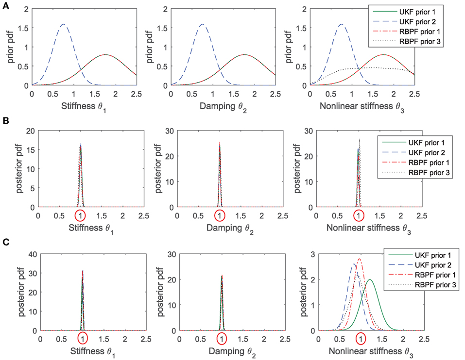
Figure 6. Performance of UKF and RBPF, with various priors, in estimating the parameters (globally identifiable) of a SDOF Duffing oscillator. (A) Prior pdfs chosen for all cases; (B) posterior pdfs, in the case where the excitation is of high amplitude and the non-linear oscillator is fully excited (plots are almost indistinguishable in this case); (C) posterior pdfs obtained in the case where the excitation is of smaller amplitude, in this case behavior of the algorithms clearly differ in their estimation of the non-linear stiffness β (∝θ₃).

Figure 6B shows results of the identification in the case where the excitation is of relatively high amplitude and the Duffing oscillator is fully excited. Recall that the posterior pdfs shown in this figure are Gaussian by construction for the UKFs, but they are a mixture of n_p Gaussians for the RBPF, with n_p = 1,000 in this case. Clearly the two algorithms perform well, and even the RBPFs yield posterior pdfs that are very close to being Gaussian. These observations agree with results presented in the study by Olivier and Smyth (2017b), where it was concluded that the assumptions made in the UKF do not negatively impact learning of the static parameters in non-linear systems in the case where parameters are identifiable and noise terms are Gaussian, in the sense that, after convergence of the parameters is achieved, the mean and variance estimates given by the UKF agree with the PF estimates. It also appears that in this case, the choice of prior pdf does not influence the posterior, which makes sense since the algorithm is able to learn from a long time series of measurements, thus somewhat forgetting prior information.

Figure 6C shows results of the identification in the case where the excitation amplitude is reduced by 80%. In this case, the linear parameters k_lin and c are still well recovered, but the UKF is unable to learn the non-linear parameter β. Its posterior pdf heavily depends on the choice of prior, which also makes sense since in this case the algorithm detects that measurements are not very informative, thus the prior knowledge has greater influence. The posterior mean obtained with a RBPF is closer to the true value, implying that in this case, the assumptions made in the UKF (Gaussianity and order of accuracy of the UT) have a negative effect on its performance. Further simulations also showed that reducing the uncertainty on the initial conditions (variance of the prior for the states) seems to help the UKF, in the sense that posterior pdfs are closer to the ones estimated with a particle filter.

For both algorithms, and for any choice of prior variance for the states (level of knowledge of the initial conditions), the posterior pdf for parameter β exhibits a large variance, meaning that the algorithm is detecting that the measurements are not informative and that uncertainty on the identified value of β is high. Thus, even though the PF performs better in this case, running a UKF (much faster) already provides some very useful information about the posterior pdf. Table 1 displays the coefficient of variation (CoV) of the parameters identified with the UKF, defined as

$\text{CoV}=\frac{\mathrm{\sigma }\left[\mathrm{\theta }|y_{1:N}\right]}{\text{E}\left[\mathrm{\theta }|y_{1:N}\right]}$ (14)

where σ[⋅] represents the standard deviation of a RV. One can observe that parameter β is not easily identified when the excitation is of small amplitude. This will be a sign for the user that the value identified with the UKF for this parameter should not be trusted and that possibly running a RBPF on these data would lead to more accurate results.

TABLE 1

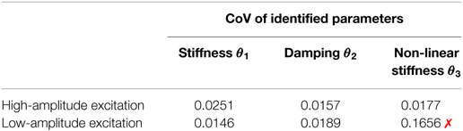
Table 1. Coefficient of variation (CoV) of the SDOF Duffing oscillator parameters identified with a UKF: when the non-linear stiffness is not excited, the UKF is not able to learn it from the measurements, which results in a CoV for this parameter much larger than for other parameters.

This issue of unidentifiability due to presence of noise and low excitations will be inherent in many real-life non-linear systems. In the study by Muto and Beck (2008), the example is given of non-linear hysteretic structures subjected to seismic event. If some parts of the structure exhibit only linear behavior during the event, no information on their yielding behavior (and associated parameters) will be available from the measurements. It is then crucial to make use of a learning algorithm that tells the user that it is not able to learn these parameters from data, as do the PF and UKF on the Duffing example described in this section. It is also important that the learning algorithm accurately estimates the posterior variance of these parameters, i.e., the posterior uncertainty on these parameters, since these estimates could be further used to estimate future behavior of the structure and quantify associated uncertainties (prognosis step).

3.2. Unidentifiable Pendulum

In the previous section, we have seen that the UKF gives useful information when it comes to noisy non-linear systems that are not highly excited. Here, we confirm this result by looking at the behavior of the UKF on an unidentifiable problem: a unit-length pendulum with rotational spring (stiffness k_rot) in free vibration, whose equation of motion is

$\ddot{\alpha }\left(t\right)=-g\cdot \mathit{sin}\left(\mathrm{\alpha }\left(t\right)\right)-\frac{k_{\mathit{rot}}}{m}\mathrm{\alpha }\left(t\right)$ (15)

where g is the known acceleration of gravity. The angle α(t) is assumed to be measured. To generate artificial noisy data, some zero-mean Gaussian noise is added to both the equation of motion (modeling error) and the measurements (measurement error). Covariances of both noise terms are assumed known when running the UKF for identification. The true values of the parameters are m = 1, k_rot = 10; we further define the vector of unknown parameters as $\mathrm{\theta }={\left[\frac{m}{1}\frac{k_{\mathit{rot}}}{10}\right]}^T$ whose true value is then ${\mathrm{\theta }}_{\mathit{true}}={\left[11\right]}^T$.

This system is clearly unidentifiable, since there exists an infinite number of vectors θ that would lead the same time series of measurements y_1:N: namely, any vector θ for which the ratio $\frac{{\mathrm{\theta }}_2}{{\mathrm{\theta }}_1}$ equates to 1.

Results of the identification procedure with the UKF are shown in Figure 7. The convergence plots show that the parameters are not identified correctly, since $\text{E}\left[\mathrm{\theta }|y_{1:N}\right]={\left[1.71.7\right]}^T\ne {\mathrm{\theta }}_{\mathit{true}}={\left[11\right]}^T$. This was expected since the system is unidentifiable. However, the standard deviation around each identified value remains very large, meaning that the algorithm is able to detect that the measurements provided are not informative enough to learn the parameters. Also, the correct ratio $\frac{{\mathrm{\theta }}_2}{{\mathrm{\theta }}_1}=1$ is identified quickly, and the posterior covariance shows a clear correlation along the line θ₁ = θ₂. Thus, the estimation procedure still provides the user with useful information about this system, i.e., θ₁ = θ₂, which was expected in this simple case.

FIGURE 7

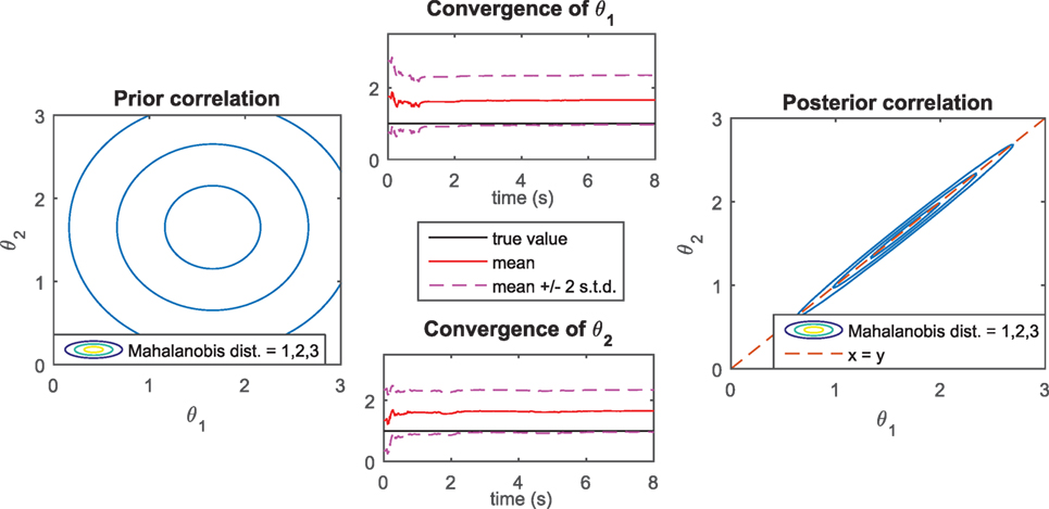
Figure 7. Pendulum with rotational spring (unidentifiable system): convergence of parameters (mean value and mean ± 2 standard deviations) and prior/posterior covariance obtained with the UKF.

3.3. Locally Identifiable System

We now consider a linear 2-DOF system, where only the second floor acceleration is measured (and the ground excitation is known/measured). This case is studied in Katafygiotis and Beck (1998), Vakilzadeh et al. (2017), and the system is shown to be locally identifiable. More specifically, defining k_lin,1 = θ₁k_lin,0 and k_lin,2 = θ₂k_lin,0, with known stiffness k_lin,0, it is shown in Katafygiotis and Beck (1998) that both vectors $\left[\begin{array}{c}\hfill {\mathrm{\theta }}_1\hfill \\ \hfill {\mathrm{\theta }}_2\hfill \end{array}\right]=\left[\begin{array}{c}\hfill 1\hfill \\ \hfill 1\hfill \end{array}\right]$ and $\left[\begin{array}{c}\hfill {\mathrm{\theta }}_1\hfill \\ \hfill {\mathrm{\theta }}_2\hfill \end{array}\right]=\left[\begin{array}{c}\hfill 2\hfill \\ \hfill 0.5\hfill \end{array}\right]$ lead to identical measurement time histories (when only the ground and second floor excitations are measured), a result that can be confirmed by running the identifiability software DAISY. The posterior pdf of $\left[\begin{array}{c}\hfill {\mathrm{\theta }}_1\hfill \\ \hfill {\mathrm{\theta }}_2\hfill \end{array}\right]$ is then expected to be multimodal, a characteristic which we know the UKF cannot handle, because of its Gaussianity assumption. Indeed Figure 8 shows two runs of the UKF (two different priors, on the same noisy data): depending on the prior chosen, the UKF will output one of the two acceptable θ_1,2³ vectors of this system, with very low posterior variance. The issue here is that if one runs only one UKF, only one outcome will be detected, with very low variance (i.e., low uncertainty on the outcome), the user will thus be given misleading information about the system.

FIGURE 8

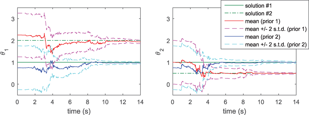
Figure 8. 2-DOF linear system: convergence of locally identifiable stiffness parameters when running two UKFs with different priors.

For this type of system, the particle filter clearly becomes the best option, since it is able to represent any type of distribution, even multimodal ones. In this case, we choose a mixture of 9 Gaussians for the prior in the [θ₁, θ₂] space, in order to have a prior which nicely explores the admissible space for these two parameters. Figure 9 shows the evolution in time of the posterior pdf in the 2-dimensional space. Clearly, the RBPF with n_p = 4,500 particles is able to approximate the true posterior, which is in this case bimodal. In Table 2, the performance of several RBPFs, with various numbers of particles, is studied with regard to both accuracy of the posterior pdf estimates (location of both modes of the posterior pdf at t_final = 14 s) and the algorithm’s running time (measured by the tic-toc function of MATLAB, for a 14 s long time series sampled at dt = 0.01 s). With only 500 particles, the RBPF is usually unable to detect the two modes. When using 1,000 particles or more (running time 7 min or more), the algorithm is able to detect and localize both modes, however, when using less than about 2,000–2,500 particles, estimates of the relative weights of each mode are very variable from run to run and quite inaccurate. A RBPF with 2,500 particles outputs consistent estimates of the posterior pdf and runs in about 18 min.

FIGURE 9

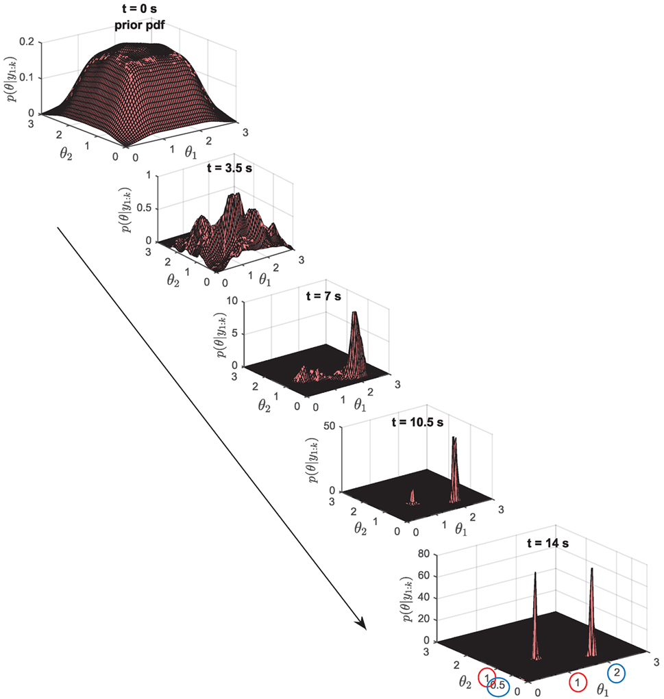
Figure 9. 2-DOF locally identifiable system: posterior pdfs p(θ|y_1:N) at different time steps k, when running a RBPF with n_p = 4,500 particles.

TABLE 2

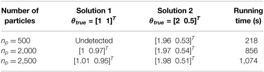
Table 2. Performance comparison of RBPFs with increasing number of particles on the 2-DOF locally identifiable system: identification of the two modes of the posterior pdf, vs. computational time.

These results were obtained assuming that the initial conditions on the states were known (the prior was given the correct mean and a small variance). Further simulations were run while relaxing this assumption, i.e., the prior for the states is given the correct mean but a larger variance, 20% RMS of the state time series, implying that there is uncertainty on the initial conditions of the system. This influences the behavior of the PF in the sense that more particles (about 3,000) are needed in this case to consistently obtain an accurate estimate of the posterior pdf. On the contrary, the UKF_GM presented in the following section, which is an enhancement of the Gaussian UKF, is more robust with regard to uncertainty on the initial conditions.

A limitation of the RBPF lies in the fact that it requires both functions f and h to be linear in the parameters [equation (8)], which is quite restrictive. For instance, it renders this algorithm impractical for systems in which the functions f, h consist of running an external program (FEM software for instance), for which it will not be possible to find such a conditionally linear partitioning. A generic bootstrap PF does not require that assumption, however it would need an enormous amount of particles to avoid degeneracy and collapse, rendering it quite inapplicable for medium to large dimensional problems. In the following section, we present an algorithm that uses some of the simplifications made in non-linear Kalman filtering schemes but allows for more complex posterior pdfs than simple Gaussians. This algorithm does not place limitations on the functions f, h, and we demonstrate that it yields very satisfactory estimates of the posterior pdfs in the numerical examples previously studied, while being computationally advantageous over a RBPF.

4. Introduction of a More Complex Non-Linear Kalman Filter

In the study by Olivier and Smyth (2017b), the authors presented a framework to derive higher order non-linear filters that would expand the scope of UKF type algorithms to non-Gaussian, possibly multimodal, distributions and thus provide a good trade-off between the accuracy of the PF and the UKF low computational complexity. The main idea is to expand the capabilities of the UKF to non-Gaussian distributions—with non-fixed higher order moments, or even multimodal distributions—while preserving the main advantages of the Kalman filter algorithms, i.e., working with an underlying distribution rather than a particle-based distribution, which facilitates the measurement update step and avoids the degeneracy issue observed in the PF. Two one-dimensional examples were given: one using a closed-skew-normal baseline distribution, the other using a mixture of Gaussians. The algorithm presented in the following sections was designed using this framework, using a non-Gaussian distribution as a baseline distribution for the pdfs of interest.

To derive a non-linear Kalman filter type algorithm in the framework previously described, one needs two components:

• a baseline distribution that is closed under conditioning to enable derivation of the measurement update equations,

• a choice of approximation to propagate the distribution and its moments through a non-linear function (Taylor series expansion, UT, or Monte Carlo simulation).

We have shown previously that for unidentifiable/locally identifiable systems: (1) the prior distribution may sometimes have a non-negligible effect on the posterior pdf and (2) the posterior pdfs might sometimes be multimodal. Using a mixture of Gaussians (GM) as a baseline distribution to a non-linear Kalman filter algorithm could thus prove useful. In the study by Olivier and Smyth (2017b), the authors proposed to use an MC approximation for propagation through non-linear functions, since the parameters of a GM distribution are usually learnt through maximum likelihood (EM algorithm). However, the EM algorithm becomes highly cumbersome in medium to large dimensional spaces. Here, we propose a different approach, which uses the unscented transform to approximate the moments of the transformed random variables. The following procedure yields a unscented Gaussian mixture filter (referred to as UKF_GM from now on), which appears to have already been studied independently in other engineering fields such as tracking (see, e.g., Faubel et al. (2009) and Luo et al. (2010)), for the purpose of dynamic state filtering in non-linear systems featuring non-Gaussian noise, possibly causing non-Gaussianity of the posterior pdfs. We quickly present the derivation of this algorithm, afterward we demonstrate its effectiveness for the purpose of parameter identification in cases where non-Gaussianity of the posterior pdfs arises from a lack of identifiability in the system.

4.1. Derivation of the UKF_GM Algorithm

4.1.1. Propagation Step

As previously mentioned, in this algorithm, the posterior pdfs are assumed to be Gaussian mixtures. Let us assume that the posterior pdf at time step k − 1 is a known mixture of L Gaussians:

$x_{k-1}\mathrm{|}{y}_{1:k-1}\sim {\displaystyle \sum _{l=1}^L}{\mathrm{\pi }}_{k-1}^{\left(l\right)}\mathcal{N}\left(\cdot ;x_{k-1|k-1}^{\left(l\right)},P_{k-1|k-1}^{\left(l\right)}\right)$ (16)

One obtains the prior at time step k by propagating this pdf through the propagation equation, which can also be written in probabilistic format as

$p\left(x_k|y_{1:k-1}\right)=\int \stackrel{\text{relates to}f}{\overbrace{p\left(x_k|x_{k-1}\right)}}p\left(x_{k-1}|y_{1:k-1}\right){\mathit{dx}}_{k-1}$ (17a)

$={\displaystyle \sum _{l=1}^L}{\mathrm{\pi }}_{k-1}^{\left(l\right)}\underset{\text{propagation of a Gaussian RV through}f}{\underbrace{\int p\left(x_k|x_{k-1}\right)\mathcal{N}\left(\cdot ;x_{k-1|k-1}^{\left(l\right)},P_{k-1|k-1}^{\left(l\right)}\right){\mathit{dx}}_{k-1}}}$ (17b)

The integral in equation (17b) represents the propagation of a Gaussian RV through the non-linear function f, which can be approximated using the UT. Applying L independent unscented transforms yields Gaussian approximations $\mathcal{N}\left(\cdot ;x_{k|k-1}^{\left(l\right)},P_{k|k-1}^{\left(l\right)}\right)$ for the integrals, and a mixture of Gaussians approximation for the prior:

$p\left(x_k|y_{1:k-1}\right)={\displaystyle \sum _{l=1}^L}{\mathrm{\pi }}_{k-1}^{\left(l\right)}\mathcal{N}\left(\cdot ;x_{k|k-1}^{\left(l\right)},P_{k|k-1}^{\left(l\right)}\right)$ (17c)

The UT is used for each Gaussian ⋅^(l) in the mixture, meaning that the total number of sigma points required for approximation of the prior pdf is N_sig = L ⋅ (2n_x + 1), if the symmetric sigma point set is used for each Gaussian. Such a sigma point set captures up to the second-order moment of the GM input RV $X=x_{k-1}|y_{1:k-1}$ (see proof in Section “Moments Captured by the Gaussian Mixture Set” in Appendix) and would achieve second-order accuracy on mean estimate and first-order accuracy on covariance estimate of the output RV $Z=f\left(X\right)=x_k|y_{1:k-1}$ (prior pdf, approximated as a GM). In this sense, this algorithm achieves the same order of accuracy as the generic UKF; however, it is now able to (1) make use of a more complex prior and (2) represent more complex pdfs, i.e., multimodal, as will be demonstrated later with a numerical example.

Before finishing the derivation of this algorithm, it is important to notice that we are making the strong assumption that each transformed Gaussian can itself be approximated as a Gaussian (same assumption as in the UKF), yielding a GM for the output RV. In the cases of highly non-linear non-Gaussian systems, this approximation might lead to erroneous results; thus, the UT should be replaced by a MC simulation, as proposed originally in the authors’ previous paper (Olivier and Smyth, 2017b). However, in the cases studied here, where multimodality arises because of lack of identifiability in the system, making use of this assumption still yields acceptable results.

4.1.2. Measurement Update Step

Regarding the measurement update step, one must first estimate the joint probability pdf of the prior and the predicted measurement, i.e., p(x_k, y_k|y_1:k−1), which is performed by transforming the prior through the measurement function h. This step can be performed in a similar fashion as for the propagation step, i.e., use independent UTs for each Gaussian constituting the prior, leading to a GM approximation of the pdf of interest as

$p\left(\left\{\begin{array}{c}\hfill x_k\hfill \\ \hfill y_k\hfill \end{array}\right\}\left|y_{1:k-1}\right.\right)\sim {\displaystyle \sum _{l=1}^L}{\mathrm{\pi }}_{k-1}^{\left(l\right)}\mathcal{N}\left(\cdot ;\left[\begin{array}{c}\hfill x_{k|k-1}^{\left(l\right)}\hfill \\ \hfill y_{k|k-1}^{\left(l\right)}\hfill \end{array}\right],\left[\begin{array}{cc}\hfill P_{k|k-1}^{\left(l\right)}\hfill & \hfill {\mathrm{\Psi }}_k^{\left(l\right)}\hfill \\ \hfill {\mathrm{\Psi }}_k^{\left(l\right),T}\hfill & \hfill S_k^{\left(l\right)}\hfill \end{array}\right]\right)$ (18)

using the same notations as in equation (11a).

The final step consists of computing the posterior pdf of the states, by conditioning the joint pdf p(x_k, y_k|y_1:k−1) over the measured value y_k. Using the closure under conditioning property of the GM distribution one can derive the following measurement update equations:

${\mathrm{\pi }}_k^{\left(l\right)}=\frac{{\mathrm{\pi }}_{k-1}^{\left(l\right)}\mathcal{N}\left(y_k;y_{k|k-1}^{\left(l\right)},S_k^{\left(l\right)}\right)}{{\sum }_{j=1}^L{\mathrm{\pi }}_{k-1}^{\left(j\right)}\mathcal{N}\left(y_k;y_{k|k-1}^{\left(j\right)},S_k^{\left(j\right)}\right)}$ (19a)

${\mathrm{\mu }}_k^{\left(l\right)}=x_{k|k-1}^{\left(l\right)}+{\mathrm{\Psi }}_k^{\left(l\right)}{\left(S_k^{\left(l\right)}\right)}^{-1}\left(y_k-y_{k|k-1}^{\left(l\right)}\right)$ (19b)

${\Sigma }_k^{\left(l\right)}=P_{k|k-1}^{\left(l\right)}-{\mathrm{\Psi }}_k^{\left(l\right)}{\left(S_k^{\left(l\right)}\right)}^{-1}{\mathrm{\Psi }}_k^{\left(l\right),T}$ (19c)

Observing these equations one sees that for each Gaussian ⋅^(l) in the mixture, the update equations are exactly the same as for a Kalman filter, or a UKF. One equation is added to the set, and consists of updating the weights π^(l) of each Gaussian, proportionally to their likelihood.

4.1.3. Treatment of Noise Terms

In the present paper, noise terms are restricted to being additive Gaussian; thus, they are introduced in the filtering equations in the exact same fashion as for a generic UKF, i.e., for each Gaussian ⋅^(l) in the mixture, the process noise covariance Q is added to the prior covariance $P_{k|k-1}^{\left(l\right)}$ at the end of the propagation step, and the measurement noise covariance R is added to the covariance of the predicted measurement $S_k^{\left(l\right)}$ before performing the measurement update. This algorithm is also able to handle non-Gaussian noise, as long as it can be represented as a mixture of Gaussians. For more details on the subject, which is outside the scope of this current paper, we refer the reader to, e.g., Faubel et al. (2009) and Luo et al. (2010).

4.2. Comments on the Algorithm and Its Computational Time

The algorithm previously presented actually reduces to running several UKFs in parallel, and weighting each UKF at each time step according to their likelihood [equation (19a)]. It is thus very easy to implement. This algorithm can be viewed as a trade-off between a UKF and a PF, in the sense that if the mixture is composed of one single Gaussian, this algorithm reduces to a generic UKF; if on the contrary the prior is composed of many Gaussians, each with an infinitely small prior covariance, the algorithm becomes very similar to a particle filter, where all particles (which can be interpreted as degenerated Gaussians) are propagated and then weighted according to their likelihood.

The overall computational time of this algorithm grows proportionally with n_x ⋅ L: it is thus proportional to both the dimension of the system and the number of Gaussians in the mixture, which governs the complexity of the pdfs of interest. If the algorithm requires highly complex Gaussian mixtures, this algorithm will then not be beneficial over a particle filter in terms of computational time. However, we have deduced from the previous numerical examples that if the parameters of the system, or at least some of them, are identifiable, then making use of a simple Gaussian prior for these parameters already yields accurate estimates. The idea in this new algorithm, when used for parameter identification purposes, is to start with a simple Gaussian prior in some of the dimensions, while using a more complex Gaussian mixture prior for the parameters that are harder to learn. Hence, the number of Gaussians in the mixture will not grow excessively with the overall dimension of the system. A more detailed comparison of the running time for the PF vs. UKF_GM is provided for the following numerical example.

4.3. Numerical Performance of the UKF_GM

4.3.1. Linear 2-DOF Locally Identifiable System

The UKF_GM is first tested on the 2-DOF locally identifiable system previously presented. The chosen prior is composed of a mixture of 49 Gaussians, leading to a quite uniform prior over the [θ₁, θ₂] space (left plot in Figure 10); however, these 49 Gaussians collapse into a single Gaussian in the remaining dimensions. The idea here is that a much more complex prior (i.e., many more Gaussians) would be necessary to uniformly explore the n_x-dimensional space, which would lead to a very computationally expensive algorithm. However, by only exploring uniformly the [θ₁, θ₂] space, one is already able to infer the multimodal posterior pdf, as shown in Figure 10 (right plot).

FIGURE 10

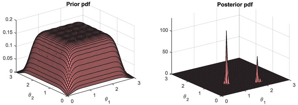
Figure 10. Performance of the UKF_GM (using a mixture of 49 Gaussians) on the 2-DOF locally identifiable system: prior and posterior pdfs of the stiffness parameters.

As previously mentioned, a tremendous advantage of the UKF_GM over the RBPF is that it does not make any assumption on the functions f, h, while the RBPF requires the functions to be linear in the parameters [equation (8)]. In this specific case for instance, the measurements were generated by running the forward problem using a 4th-order Runge–Kutta discretization scheme. However, learning the parameters with the RBPF requires the writing of the function f using an Euler discretization scheme. When running the UKF_GM on the contrary, we were able to use a Runge–Kutta discretization scheme for the function f, i.e., the model used to run the inverse problem is closer to the true system.

In Table 3, performance of this algorithm, using two different sigma point sets (the symmetric set and the simplex spherical set, both plotted on Figure 5), is analyzed in terms of accuracy of the posterior pdfs and running time, as done previously for the PF. One can see that the UKF_GM is able to quite accurately identify the two modes of the posterior pdf, and does so with a reduced computational time compared to a RBPF. This can be explained by looking more precisely at the computational effort required for each algorithm. For the RBPF, the main computational load originates from evaluating $f\left(x_{k-1}^{\left(i\right)},{\mathrm{\theta }}^{\left(i\right)}\right)$, $h\left(x_k^{\left(i\right)},{\mathrm{\theta }}^{\left(i\right)}\right)$ as well as performing two linear measurement update equations (to update the conditional pdf of the conditionally linear parameters), and so for each particle. Regarding the UKF_GM, for each of the N_sig sigma points, with N_sig = 833 for the symmetric set and N_sig = 490 for the simplex set, the main computational load originates solely from evaluating $f\left(x_{k-1}^{\left(i\right)},{\mathrm{\theta }}^{\left(i\right)}\right)$, $h\left(x_k^{\left(i\right)},{\mathrm{\theta }}^{\left(i\right)}\right)$, then only L measurement updates are needed per time step. This algorithm thus reduces computational time in two ways compared to the RBPF: reduce the number of particles/sigma points per time step and reduce the computational time per particle/sigma point (for the same function f).

TABLE 3

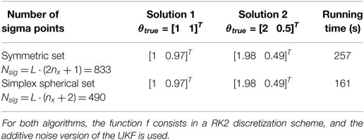
Table 3. Performance comparison of the UKF_GM with two sigma point sets on the 2-DOF locally identifiable system: identification of the two modes of the posterior pdf vs. computational time.

The number of mixtures in the GM is chosen in advance by the user. This number should not be chosen too small for two reasons: (1) having a complex prior enables a good coverage of the prior parameter space, which is required in order to detect all possible parameter solutions and (2) we have observed in our experiments that if only few Gaussians are considered, the algorithm tends to collapse as in a PF, i.e., one Gaussian will be given all the weight and the posterior pdf will be Gaussian.

4.3.2. Duffing Oscillator

The performance of the UKF_GM was also assessed on the Duffing oscillator problem previously considered, in the case where the non-linearity is not fully excited. Recall that in this case, the UKF is not able to accurately learn the non-linear stiffness parameter α. Very importantly, comparing behaviors of UKFs with different priors seems to indicate that the chosen prior has a non-negligible influence on the posterior. It is thus important in this case to be able to accurately represent the level of prior knowledge with a proper prior distribution. For this test, we chose again as prior pdf a mixture of 49 Gaussians, which explores quite uniformly the 2-dimensional [θ₁, θ₃] ∝ [k, α] space (since the two stiffness parameters are correlated, the algorithm yields much better results when this 2-dimensional space is explored uniformly, rather than just the θ₃ dimension). Both the prior and posterior distributions are shown in Figure 11, demonstrating the ability of this new algorithm to learn the posterior value of α in a more accurate way than a single UKF, while still yielding a large variance for this parameter, indicating that measurements are not very informative in this case.

FIGURE 11

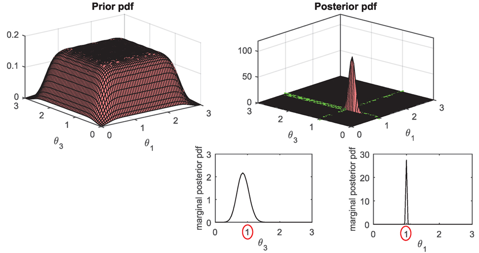
Figure 11. Performance of the UKF_GM (using a mixture of 49 Gaussians) on the SDOF Duffing oscillator (low amplitude excitation): prior and posterior pdfs of the linear and non-linear stiffness parameters, θ₁ ∝ k_lin and θ₃ ∝ β.

5. Conclusion

The contributions of this paper are twofold. First, the behavior of online Bayesian inference algorithms for parameter identification of systems that exhibit various identifiability characteristics was studied. The question of parameter identifiability, i.e., whether there is a unique solution to the inverse problem, will influence the choice of algorithm used to perform identification.

• For the identifiable systems considered in this paper (non-linear systems with Gaussian noise), the UKF performs very well in estimating the posterior pdf of the parameters and is very attractive due to its low computational cost,

• for unidentifiable parameters (noise-free unidentifiability or unidentifiability due to presence of noise), the UKF still gives very useful information on the system, more particularly on the posterior covariance characteristics, but a PF should be used in order to obtain a better approximation of the true posterior pdf,

• for locally identifiable systems, the particle filter will be able to detect the multimodality of the posterior pdf, with the condition that enough particles are used for the approximation, and it will possibly do so relatively fast compared to MCMC or other offline techniques.

This issue of parameter identifiability will become of vital importance for real life, large dimensional, high fidelity models since the number of unknown parameters will surely increase; however, the number of measurements might not be allowed to augment proportionally, for practical reasons. A challenge in high fidelity models (finite element models for instance) lies in the choice of the parameter vector to be learnt from data (engineering judgment vs. sensitivity-based methods (Jang and Smyth, 2017) for instance), and then to assess the identifiability of this parameter vector. In this paper, small-scale problems were studied, whose system equations f and h were easy to write, thus enabling assessment of the systems identifiability properties prior to learning, through the use of identifiability tests such as the DAISY software. Running identifiability tests on large dimensional problems, described by FE models, would be much more challenging. Thus, for large-scale systems, identifiability characteristics of the parameter vector might not be known in advance, it is then of primordial importance to understand how online algorithms perform in order to accurately analyze and understand the results of the identification task. Part of the authors’ foreseen work relates to applying these online methods to full-scale FEM problems, which would require further algorithmic improvements in order to reduce the computational cost and enable real-time monitoring.

The second objective of this paper was to show the applicability and computational efficiency of an unscented Kalman filter that uses a Gaussian mixture as baseline distribution on this type of challenging problem. As previously stated, the UKF presents a tremendous advantage compared to MC techniques (PF, MCMC) in the sense that its overall computational time is only linearly proportional to the size of the state vector. It should, however, be used with caution when the system of interest presents challenging identifiability properties (local identifiability or unidentifiability), or non-Gaussian noise terms (topic partially discussed in the study by Olivier and Smyth (2017b)). In the second part of the paper, we thus presented a more complex non-linear unscented Kalman filter, which makes use of some of the attractive simplifications of the UKF, and is thus computationally efficient, while allowing for more complex posterior distributions (Gaussian mixtures). We demonstrate its capabilities with regard to identification of parameters, even in cases where the posterior pdf is multimodal (locally identifiable system). Additionally, this algorithm possesses the additional advantages that no assumption is made on the functions f, h; and that more complex noise terms (Gaussian mixtures) could be introduced.

Overall this paper demonstrates that online algorithms have excellent capabilities regarding joint state/parameter estimation, even when the lack of identifiability of the system causes the posterior pdfs to be non-Gaussian, multimodal. Furthermore, these algorithms make use at each time step of independent evaluations of the functions f, h at various points in the state space, they are thus quite easily parallelizable [see, e.g., Brun et al. (2002) for PF parallelization], making them very attractive for real-time monitoring of systems. This further enables fast decision-making procedures, very important in the case of structural health monitoring. Also, these first posterior estimates could be used to speed up offline methods such as MCMC schemes, by using them as starting point or as importance densities in the case of importance sampling, thus yielding more accurate estimates of the posterior pdfs.

Author Contributions

Both authors (AO and AS) contributed to the research, numerical simulations presented in the paper, and writing of the manuscript.

Conflict of Interest Statement

The authors declare that the research was conducted in the absence of any commercial or financial relationships that could be construed as a potential conflict of interest.

Acknowledgments

The authors would like to thank Manolis Chatzis for his help regarding the use of identifiability tests and more particularly the DAISY software.

Funding

The authors would also like to acknowledge the support of the U.S. National Science Foundation, which partially supported this research under Grant Nos. CMMI-1100321 and CMMI-1563364.

Footnotes

1. ^We however introduce a small modeling error by using a different discretization scheme when generating the data (Runge–Kutta, order 4), vs. running the inverse problem (Euler or RK order 2). This type of modeling error will be inherent in any real-life system.
2. ^Olivier, A., and Smyth, A. W. (2017). Damage detection through nonlinear filtering for systems subjected to unmeasured wind excitation whose spectral properties are known but uncertain. Mech. Syst. Signal Process. (Under Review).
3. ^In this problem, the damping parameters are also assumed unknown, so the size of the parameter vector is 4; however, we focus our attention on the locally identifiable parameters θ_1,2.

References

Ang, A. H.-S., and Tang, W. H. (2007). Probability Concepts in Engineering: Emphasis on Applications to Civil and Environmental Engineering, 2nd Edn. Hoboken, NJ: John Wiley & Sons, Inc.

Google Scholar

ASCE. (2016). 2013 Report Card for America’s Infrastructure. Available at: http://www.infrastructurereportcard.org

Google Scholar

Beck, J. L., and Au, S.-K. (2002). Bayesian updating of structural models and reliability using Markov chain Monte Carlo simulation. J. Eng. Mech. 128, 380–391. doi:10.1061/(ASCE)0733-9399(2002)128:4(380)

CrossRef Full Text | Google Scholar

Beck, J. L., and Zuev, K. M. (2013). Asymptotically independent Markov sampling: a new Markov Chain Monte Carlo scheme for Bayesian inference. Int. J. Uncertain. Quantif. 3, 445–474. doi:10.1615/Int.J.UncertaintyQuantification.2012004713

CrossRef Full Text | Google Scholar

Bellu, G., Pia Saccomani, M., Audoly, S., and D’Angiò, L. (2007). DAISY: a new software tool to test global identifiability of biological and physiological systems. Comput. Methods Programs Biomed. 88, 52–61. doi:10.1016/j.cmpb.2007.07.002

PubMed Abstract | CrossRef Full Text | Google Scholar

Bengtsson, T., Bickel, P., and Li, B. (2008). “Curse-of-dimensionality revisited: collapse of the particle filter in very large scale systems,” in Probability and Statistics: Essays in Honor of David A. Freedman, Vol. 2 (Beachwood, OH, USA: Institute of Mathematical Statistics), 316–334. doi:10.1214/193940307000000518

CrossRef Full Text | Google Scholar

Brun, O., Teuliere, V., and Garcia, J.-M. (2002). Parallel particle filtering. J. Parallel Distrib. Comput. 62, 1186–1202. doi:10.1006/jpdc.2002.1843

CrossRef Full Text | Google Scholar

Cappé, O., Godsill, S. J., and Moulines, E. (2007). “An overview of existing methods and recent advances in sequential Monte Carlo,” in Proceedings of the IEEE, Vol. 95, 899–924. doi:10.1109/JPROC.2007.893250

CrossRef Full Text | Google Scholar

Chatzis, M., Chatzi, E., and Smyth, A. (2015). On the observability and identifiability of nonlinear structural and mechanical systems. Struct. Control Health Monit. 22, 574–593. doi:10.1002/stc.1690

CrossRef Full Text | Google Scholar

Ching, J., and Chen, Y. (2007). Transitional Markov chain Monte Carlo method for Bayesian model updating, model class selection, and model averaging. J. Eng. Mech. 133, 816–832. doi:10.1061/(ASCE)0733-9399(2007)133:7(816)

CrossRef Full Text | Google Scholar

Crisan, D., and Doucet, A. (2002). A survey of convergence results on particle filtering methods for practitioners. IEEE Trans. Signal Process. 50, 736–746. doi:10.1109/78.984773

CrossRef Full Text | Google Scholar

Doucet, A., de Freitas, N., Murphy, K. P., and Russell, S. J. (2000). “Rao-Blackwellised particle filtering for dynamic Bayesian networks,” in UAI’00: Proceedings of the 16th Conference on Uncertainty in Artificial Intelligence (San Francisco, CA: Morgan Kaufmann Publishers Inc.), 176–183.

Google Scholar

Doucet, A., and Johansen, A. M. (2011). “A tutorial on particle filtering and smoothing: fifteen years later,” in The Oxford Handbook of Nonlinear Filtering, eds D. Crisan and B. Rozovskii (New York: Oxford University Press Inc.), 656–704.

Google Scholar

Dubbs, N. C., and Moon, F. L. (2015). Comparison and implementation of multiple model structural identification methods. J. Struct. Eng. 141, 04015042. doi:10.1061/(ASCE)ST.1943-541X.0001284

CrossRef Full Text | Google Scholar

Faubel, F., McDonough, J., and Klakow, D. (2009). The split and merge unscented Gaussian mixture filter. IEEE Signal Process. Lett. 16, 786–789. doi:10.1109/LSP.2009.2024859

CrossRef Full Text | Google Scholar

Green, P. L. (2015). Bayesian system identification of a nonlinear dynamica system using a novel variant of simulated annealing. Mech. Syst. Signal Process. 52–53, 133–146. doi:10.1016/j.ymssp.2014.07.010

CrossRef Full Text | Google Scholar

Jang, J. (2016). Development of Data Analytics and Modeling Tools for Civil Infrastructure Condition Monitoring Applications. Ph.D. thesis, Columbia University Academic Commons, New York.

Google Scholar

Jang, J., and Smyth, A. W. (2017). Model updating of a full-scale FE model with nonlinear constraint equations and sensitivity-based cluster analysis for updating parameters. Mech. Syst. Signal Process. 83, 337–355. doi:10.1016/j.ymssp.2016.06.018

CrossRef Full Text | Google Scholar

Julier, S. J., and Uhlmann, J. K. (1997). A consistent, debiased method for converting between polar and Cartesian coordinate systems. SPIE Proc. 3086, 110–121. doi:10.1117/12.277178

CrossRef Full Text | Google Scholar

Julier, S. J. (1998). “Skewed approach to filtering,” in Proc. SPIE 3373, Signal and Data Processing of Small Targets, Vol. 3373 (Orlando, FL), 271–282. doi:10.1117/12.324626

CrossRef Full Text | Google Scholar

Julier, S. J. (2002). “The scaled unscented transformation,” in Proceedings of the 2002 American Control Conference, Vol. 6 (Anchorage, AK: IEEE), 4555–4559. doi:10.1109/ACC.2002.1025369

CrossRef Full Text | Google Scholar

Julier, S. J., and Uhlmann, J. K. (2002). “Reduced sigma point filters for the propagation of means and covariances through nonlinear transformations,” in Proceedings of the 2002 American Control Conference, Vol. 2 (Anchorage, AK: IEEE), 887–892. doi:10.1109/ACC.2002.1023128

CrossRef Full Text | Google Scholar

Julier, S. J., and Uhlmann, J. K. (2004). Unscented filtering and nonlinear estimation. Proc. IEEE 92, 401–422. doi:10.1109/JPROC.2003.823141

CrossRef Full Text | Google Scholar

Katafygiotis, L. S., and Beck, J. L. (1998). Updating models and their uncertainties. II: model identifiability. J. Eng. Mech. 124, 463–467. doi:10.1061/(ASCE)0733-9399(1998)124:4(463)

CrossRef Full Text | Google Scholar

Kontoroupi, T., and Smyth, A. W. (2016). Online noise identification for joint state and parameter estimation of nonlinear systems. ASCE ASME J. Risk Uncertain. Eng. Syst. A Civ. Eng. 2, B4015006. doi:10.1061/AJRUA6.0000839

CrossRef Full Text | Google Scholar

Kontoroupi, T., and Smyth, A. W. (2017). Online Bayesian model assessment using nonlinear filters. Struct. Control Health Monit. 24, e1880. doi:10.1002/stc.1880

CrossRef Full Text | Google Scholar

Lindsten, F. (2013). “An efficient stochastic approximation EM algorithm using conditional particle filters,” in IEEE International Conference on Acoustics, Speech and Signal Processing (Vancouver, BC: IEEE), 6274–6278. doi:10.1109/ICASSP.2013.6638872

CrossRef Full Text | Google Scholar

Luo, X., Moroz, I. M., and Hoteit, I. (2010). Scaled unscented transform Gaussian sum filter: theory and application. Physica D: Nonlinear Phenomena 239, 684–701. doi:10.1016/j.physd.2010.01.022

CrossRef Full Text | Google Scholar

Muto, M., and Beck, J. L. (2008). Bayesian updating and model class selection for hysteretic structural models using stochastic simulation. J. Vibr. Control 14, 7–34. doi:10.1177/1077546307079400

CrossRef Full Text | Google Scholar

Olivier, A., and Smyth, A. W. (2017a). Particle filtering and marginalization for parameter identification in structural systems. Struct. Control Health Monit. 24, e1874. doi:10.1002/stc.1874

CrossRef Full Text | Google Scholar

Olivier, A., and Smyth, A. W. (2017b). Review of nonlinear filtering for SHM with an exploration of novel higher order Kalman filtering algorithms for uncertainty quantification. J. Eng. Mech. doi:10.1061/(ASCE)EM.1943-7889.0001276

CrossRef Full Text | Google Scholar

Özkan, E., Šmídl, V., Saha, S., Lundquist, C., and Gustafsson, F. (2013). Marginalized adaptive particle filtering for nonlinear models with unknown time- varying noise parameters. Automatica 49, 1566–1575. doi:10.1016/j.automatica.2013.02.046

CrossRef Full Text | Google Scholar

Pasquier, R., and Smith, I. F. C. (2016). Iterative structural identification framework for evaluation of existing structures. Eng. Struct. 106, 179–194. doi:10.1016/j.engstruct.2015.09.039

CrossRef Full Text | Google Scholar

Poyiadjis, G., Singh, S. S., and Doucet, A. (2006). “Gradient-free maximum likelihood parameter estimation with particle filters,” in Proceedings of the 2006 American Control Conference (Minneapolis, MN: IEEE), 3062–3067. doi:10.1109/ACC.2006.1657187

CrossRef Full Text | Google Scholar

Rebeschini, P., and van Handel, R. (2015). Can local particle filters beat the curse of dimensionality? Ann. Appl. Probab. 25, 2809–2866. doi:10.1214/14-AAP1061

CrossRef Full Text | Google Scholar

Rytter, A. (1993). Vibrational Based Inspection of Civil Engineering Structures. Ph.D. thesis, Department of Building Technology and Structural Engineering, Aalborg University, Aalborg, Denmark.

Google Scholar

Särkkä, S. (2013). Bayesian Filtering and Smoothing. New York, NY: Cambridge University Press.

Google Scholar

Schön, T., Gustafsson, F., and Nordlund, P.-J. (2005). “Marginalized particle filters for mixed linear/nonlinear state-space models,” in IEEE Transactions on Signal Processing, Vol. 53, 2279–2289. doi:10.1109/TSP.2005.849151

CrossRef Full Text | Google Scholar

Smith, R. C. (2014). Uncertainty Quantification: Theory, Implementation, and Applications. Philadelphia, PA: Society for Industrial and Applied Mathematics.

Google Scholar

Vakilzadeh, M. K., Huang, Y., Beck, J. L., and Abrahamsson, T. (2017). Approximate Bayesian Computation by Subset Simulation using hierarchical state-space models. Mech. Syst. Signal Process. 84, 2–20. doi:10.1016/j.ymssp.2016.02.024

CrossRef Full Text | Google Scholar

Wan, E. A., and Van Der Merwe, R. (2000). “The unscented Kalman filter for nonlinear estimation,” in Proceedings of the IEEE 2000 Adaptive Systems for Signal Processing, Communications, and Control Symposium 2000. AS-SPCC (Lake Louise: IEEE), 153–158. doi:10.1109/ASSPCC.2000.882463

CrossRef Full Text | Google Scholar

Appendix

A. Moments Captured by the Gaussian Mixture Set

Let us consider an input RV X, known to be distributed as a mixture of L Gaussians

$X\sim {\displaystyle \sum _{l=1}^L}{\mathrm{\pi }}^{\left(l\right)}\mathcal{N}\left(\cdot ;{\mathrm{\mu }}^{\left(l\right)},{\Sigma }^{\left(l\right)}\right)$

In this section, we show that a sigma point set composed of L symmetric sets, one for each Gaussian ⋅^(l) in the mixture, weighted according to the mixture weights π^(l), captures the mean and covariance of the GM input RV X. This set will then achieve second-order accuracy on estimation of the mean of a transformed RV Z = g(X), and first-order accuracy on the covariance estimation.

We define the set of N_sig = L ⋅ (2n_x + 1) sigma points ${\left\{{\mathcal{X}}^{\left(i,l\right)}\right\}}_{i=0:2n_x,l=1:L}$ and their associated weights ${\left\{W^{\left(i,l\right)}\right\}}_{i=0:2n_x,l=1:L}$ as

$\begin{array}{l}\forall l\in \left[1:L\right],\hfill \\ {\mathcal{X}}^{\left(0,l\right)}={\mathrm{\mu }}^{\left(l\right)}{W}^{\left(0,l\right)}={\mathrm{\pi }}^{\left(l\right)}{w}^{\left(0\right)}\hfill \\ {\mathcal{X}}^{\left(i,l\right)}={\mathrm{\mu }}^{\left(l\right)}+\sqrt{\mathrm{\kappa }+n_x}{\left(\sqrt{{\Sigma }^{\left(l\right)}}\right)}_i{W}^{\left(i,l\right)}={\mathrm{\pi }}^{\left(l\right)}{w}^{\left(i\right)},\text{for}i=1:n_x\hfill \\ {\mathcal{X}}^{\left(n_x+i,l\right)}={\mathrm{\mu }}^{\left(l\right)}-\sqrt{\mathrm{\kappa }+n_x}{\left(\sqrt{{\Sigma }^{\left(l\right)}}\right)}_i{W}^{\left(i,l\right)}={\mathrm{\pi }}^{\left(l\right)}{w}^{\left(n_x+i\right)},\text{for}i=1:n_x\hfill \end{array}$

where ${\left\{w^{\left(i\right)}\right\}}_{i=0:2n_x}$ are the weights associated with the symmetric set. For each Gaussian in the mixture, the symmetric set captures mean and covariance of the input Gaussian ⋅^(l) by construction, i.e.,

$\begin{array}{l}{\displaystyle \sum _{i=0}^{2n_x}}{w}^{\left(i\right)}{\mathcal{X}}^{\left(i,l\right)}={\mathrm{\mu }}^{\left(l\right)}\hfill \\ {\displaystyle \sum _{i=0}^{2n_x}}{w}^{\left(i\right)}\left({\mathcal{X}}^{\left(i,l\right)}-{\mathrm{\mu }}^{\left(l\right)}\right){\left({\mathcal{X}}^{\left(i,l\right)}-{\mathrm{\mu }}^{\left(l\right)}\right)}^T={\Sigma }^{\left(l\right)}\hfill \end{array}$

Then, we show that the total set captures the global mean and covariance of the RV X (mixture of L Gaussians). Derivation for the mean is as follows:

$\begin{array}{l}{\displaystyle \sum _{l=1}^L}{\displaystyle \sum _{i=0}^{2n_x}}{W}^{\left(i,j\right)}{\mathcal{X}}^{\left(i,l\right)}={\displaystyle \sum _{l=1}^L}{\mathrm{\pi }}^{\left(l\right)}{\displaystyle \sum _{i=0}^{2n_x}}{w}^{\left(i\right)}{\mathcal{X}}^{\left(i,l\right)}\hfill \\ ={\displaystyle \sum _{l=1}^L}{\mathrm{\pi }}^{\left(l\right)}{\mathrm{\mu }}^{\left(l\right)}\hfill \\ =\text{E}\left[X\right]\left(\text{equation for mean of a Gaussian mixture}\right)\hfill \end{array}$

and for the covariance:

$\begin{array}{l}{\displaystyle \sum _{l=1}^L}{\displaystyle \sum _{i=0}^{2n_x}}{W}^{\left(i,j\right)}\left({\mathcal{X}}^{\left(i,l\right)}-\text{E}\left[X\right]\right){\left({\mathcal{X}}^{\left(i,l\right)}-\text{E}\left[X\right]\right)}^T\hfill \\ ={\displaystyle \sum _{l=1}^L}{\mathrm{\pi }}^{\left(l\right)}{\displaystyle \sum _{i=0}^{2n_x}}{w}^{\left(i\right)}\left({\mathcal{X}}^{\left(i,l\right)}-{\mathrm{\mu }}^{\left(l\right)}+{\mathrm{\mu }}^{\left(l\right)}-\text{E}\left[X\right]\right){\left({\mathcal{X}}^{\left(i,l\right)}-{\mathrm{\mu }}^{\left(l\right)}+{\mathrm{\mu }}^{\left(l\right)}-\text{E}\left[X\right]\right)}^T\hfill \\ ={\displaystyle \sum _{l=1}^L}{\mathrm{\pi }}^{\left(l\right)}{\displaystyle \sum _{i=0}^{2n_x}}{w}^{\left(i\right)}\left(\left({\mathcal{X}}^{\left(i,l\right)}-{\mathrm{\mu }}^{\left(l\right)}\right){\left({\mathcal{X}}^{\left(i,l\right)}-{\mathrm{\mu }}^{\left(l\right)}\right)}^T+\left({\mathrm{\mu }}^{\left(l\right)}-\text{E}\left[X\right]\right){\left({\mathrm{\mu }}^{\left(l\right)}-\text{E}\left[X\right]\right)}^T\right)\hfill \\ +{\displaystyle \sum _{l=1}^L}{\mathrm{\pi }}^{\left(l\right)}{\displaystyle \sum _{i=0}^{2n_x}}{w}^{\left(i\right)}\left(\left({\mathcal{X}}^{\left(i,l\right)}-{\mathrm{\mu }}^{\left(l\right)}\right){\left({\mathrm{\mu }}^{\left(l\right)}-\text{E}\left[X\right]\right)}^T\right.\left.+\left({\mathrm{\mu }}^{\left(l\right)}-\text{E}\left[X\right]\right){\left({\mathcal{X}}^{\left(i,l\right)}-{\mathrm{\mu }}^{\left(l\right)}\right)}^T\right)\hfill \end{array}$

The two last terms of this 4 terms sum can be shown to equate to 0, which is shown as

$\begin{array}{l}{\displaystyle \sum _{i=0}^{2n_x}}{w}^{\left(i\right)}\left({\mathcal{X}}^{\left(i,l\right)}-{\mathrm{\mu }}^{\left(l\right)}\right){\left({\mathrm{\mu }}^{\left(l\right)}-\text{E}\left[X\right]\right)}^T=\left(\left({\displaystyle \sum _{i=0}^{2n_x}}{w}^{\left(i\right)}{\mathcal{X}}^{\left(i,l\right)}\right)-{\mathrm{\mu }}^{\left(l\right)}\right){\left({\mathrm{\mu }}^{\left(l\right)}-\text{E}\left[X\right]\right)}^T\hfill \\ =\left({\mathrm{\mu }}^{\left(l\right)}-{\mathrm{\mu }}^{\left(l\right)}\right){\left({\mathrm{\mu }}^{\left(l\right)}-\text{E}\left[X\right]\right)}^T\hfill \\ =0\hfill \end{array}$

which then gives for the covariance:

$\begin{array}{l}{\displaystyle \sum _{l=1}^L}{\displaystyle \sum _{i=0}^{2n_x}}{W}^{\left(i,j\right)}\left({\mathcal{X}}^{\left(i,l\right)}-\text{E}\left[X\right]\right){\left({\mathcal{X}}^{\left(i,l\right)}-\text{E}\left[X\right]\right)}^T\hfill \\ ={\displaystyle \sum _{l=1}^L}{\mathrm{\pi }}^{\left(l\right)}{\displaystyle \sum _{i=0}^{2n_x}}{w}^{\left(i\right)}\left(\left({\mathcal{X}}^{\left(i,l\right)}-{\mathrm{\mu }}^{\left(l\right)}\right){\left({\mathcal{X}}^{\left(i,l\right)}-{\mathrm{\mu }}^{\left(l\right)}\right)}^T\right.\left.+\left({\mathrm{\mu }}^{\left(l\right)}-\text{E}\left[X\right]\right){\left({\mathrm{\mu }}^{\left(l\right)}-\text{E}\left[X\right]\right)}^T\right)\hfill \\ ={\displaystyle \sum _{l=1}^L}{\mathrm{\pi }}^{\left(l\right)}\left({\Sigma }^{\left(l\right)}+\left({\mathrm{\mu }}^{\left(l\right)}-\text{E}\left[X\right]\right){\left({\mathrm{\mu }}^{\left(l\right)}-\text{E}\left[X\right]\right)}^T\right)\hfill \\ =\mathit{Cov}\left(X\right)\left(\text{equation for covariance of a Gaussian mixture}\right)\hfill \end{array}$