Vibration Monitoring of Gas Turbine Engines: Machine-Learning Approaches and Their Challenges

Introduction

Vibration measurements are commonly considered to be a sound indicator of a machine’s overall health state (global monitoring). The general principle behind using vibration data is that when faults start to develop, the system dynamics change, which results in different vibration patterns from those observed at the healthy state of the system monitored. In recent years, gas turbine engine manufacturers have turned their attention into increasing the reliability and availability of their fleet using data-driven vibration-based condition monitoring approaches (King et al., 2009). These methods are generally preferred, for online monitoring strategies, over a physics-based modeling approach, where a generic theoretical model is developed and in which several assumptions surround its development. In the case of data-driven condition monitoring approaches, a model based on engine data can be constructed so that inherent linear and non-linear relationships, depending on the method, that are specific to the system being monitored, can be captured. For this reason, engine manufacturers see the need to implement such approaches during pass-off tests, where it is necessary to identify possible defects at an early stage, before complete component failure occurs.

Due to the complex processes taking place in a gas turbine engine, and since modes of failure of such systems are rarely observed in practice, the novelty detection paradigm is normally adopted for developing a data-driven model (Tarassenko et al., 2009), since in this case only data coming from the healthy state of the system are needed for training. On the other hand, conventional multi-class classification approaches are not as easy to implement, since it is not possible to have data and/or understanding (labels) from all classes of failure. The main concept of a novelty detection method is described Pimentel et al. (2014): training data from one class are used to construct a data-driven model describing the distribution they belong to. Data that do not belong to this class are novel/outliers. In a gas turbine engine context, a model of “normal” engine condition (class 𝒩) is developed, since data are only available from this class. This model is then used to determine whether new unseen data points are classed as normal or “novel” (class 𝒜), by comparing them with the distribution learned from class 𝒩 data. Such a model must be sensitive enough to identify potential precursors of localized component malfunctioning at a very early stage that can lead to total engine failure. The costs of a run-to-break maintenance strategy (i.e., decommissioning equipment after failure for replacement) are exceptionally high, but most importantly safety requirements are crucial, and thus, robust alarming mechanisms are required in such systems.

Novelty detection approaches exploit machine learning and statistics. In this study, we will use a non-parametric approach that is specific to the engine being monitored and relies solely on the data for developing the model. The novelty detection field comprises a large portion of the machine-learning discipline and therefore, only a few examples of literature, specific to the application of engine condition monitoring using machine learning, will be mentioned here. Some of the earliest works in this field were made possible through collaboration between Oxford University and Rolls Royce (Hayton et al., 2000). The authors in that paper have used data from vibrations to train a one-class support vector machine (OCSVM). The so-called tracked orders (defined as the vibration amplitudes centered at the fundamental of engine shaft speed and its harmonics) were used as training features for the OCSVM. The OCSVM has also been implemented to detect the impending combustion instability in industrial combustor systems using combustion pressure measurements and combustion high-speed images as input training data (Clifton et al., 2007). The method has also been extended in Clifton et al. (2014) to calibrate the novelty scores of the OCSVM into conditional probabilities.

The choice of the kernel function used in the OCSVM influences its classification accuracy significantly. Since a kernel defines the similarity between two points, its choice is mainly dependent on the data. However, the kernel width is a more important factor than the particular kernel function choice since it can be selected in a manner that ensures that the data are described in the best way possible (Scholkopf and Smola, 2001). Although kernel methods are considered as a good way of injecting domain specific knowledge in an algorithm like the OCSVM, the kernel function choice and its parameters’ tuning is not so straightforward. In this study, the authors follow a relatively simple approach to determine both the kernel function parameter and the optimization penalty parameter for the OCSVM. The kernel function parameter that was varied is the radial basis function (RBF) kernel width γ, together with the optimization penalty parameter ν. In general, γ controls the complexity of describing the training examples, while ν defines the upper bound on the fraction of training data points that are outside the boundary defined for class 𝒩 data. Using these two parameters, a compromise can be made between good model generalization capability and good description of the data (training data set) to obtain accurate and reliable predictions.

The novelty detection scheme that is presented in the following sections has been developed for a gas turbine engine that operates on a range of alternative fuels on different air-to-fuel ratios. This engine is being used to study the influence of such operating parameters on its performance (e.g., exhaust emissions), and thus, it is important to enable the early detection of impending faults that might take place during these tests. Since we apply novelty detection on a global system basis, the whole frequency spectrum of vibration must be used for monitoring, rather than specific frequency bands that correspond to engine components. As will be shown later, large vibration amplitudes can be expected in any region along the spectrum.

Experimental Setup and Data Description

The experimental data used in this work were taken from a larger project that aimed to characterize different alternative fuels from an engine performance perspective, e.g., fuel consumption and exhaust emissions. Alternative fuels that are composed of conventional kerosene-based fuel Jet-A1 and bio jet fuels have shown promising results in terms of reducing greenhouse gas emissions and other performance indicators. Several research programs studied alternative fuels for aviation quite extensively, as reviewed in Blakey et al. (2011). The facility that was used to test the different alternative fuels under different engine air-to-fuel ratios, houses a Honeywell GTCP85-129, which is an auxiliary power unit of turboshaft gas turbine engine type. Thus, the operating principle of this engine follows a typical Brayton cycle. As can be shown in the schematic diagram of the engine in Figure 1, the engine draws ambient air from the inlet (1 atm) through the centrifugal compressor C1, where it raises its pressure by accelerating the fluid and passing it through a divergent section. The fluid pressure is further increased across a second centrifugal compressor C2, before being mixed with fuel into the combustion chamber (CC) and ignited to add energy into the system (in the form of heat) at constant pressure. The high temperature and pressure gasses are expanded across the turbine, which drives the two compressors, a 32 kW generator G that provides aircraft electrical power and the engine accessories (EA), e.g., fuel pumps, through a speed reduction gearbox.

FIGURE 1

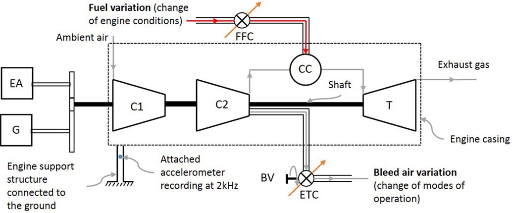
Figure 1. Gas turbine engine schematic diagram of the experimental unit, depicting salient features.

The bleed valve (BV) of the engine, allows the extraction of high temperature, compressed air (~232°C at 338 kPa of absolute pressure) to be passed to the aircraft cabin and to provide pneumatic power to start the main engines. This allows the engine to be tested on different operating modes as the air-to-fuel mass flow that goes into the CC can be changed with the BV position. When the BV opens, a decrease in turbine speed will take place if there is no addition of fuel to compensate for the lost work. The energy loss arises from the decrease in work done w_c2 to the engine’s working fluid as it passes through the second compression stage. The amount of lost work is proportional to the extracted bleed air mass m_bleed and can be expressed as w_c2 = m_bleed c_pdT, with c_p representing the heat capacity of the working fluid and dT the temperature differential across the second compression stage. Since the shaft speed must remain constant at 4,356 ± 10.5 rad/s, the fuel flow controller achieves this by regulating the pressure in the fuel line, by injecting different mass fuel flow into the CC.

Increasing the fuel mass flow that goes into the CC to maintain constant shaft speed without a subsequent increase in air mass flow rate, raises the exhaust gas temperature, as can be shown in Table 1. This can be explained by the fact that when there is a deficiency of oxygen required for complete combustion of the incoming sprayed fuel, more droplets of fuel are carried further downstream of the CC, until they eventually burn. This gradual burning of fuel along the combustion section causes the associated flame to propagate further toward the dilution zone. Hence, inadequate cooling of the gas stream takes place, which causes higher combustor exit and, in turn, exhaust gas temperatures. This also implies that there is an upper and lower limit for the exhaust gas temperature, which is monitored and controlled by the electronic temperature controller.

TABLE 1

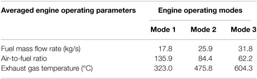
Table 1. Averaged engine operating parameters for three operating modes on Jet-A1 fuel.

Three operating modes have been considered by changing the BV on three positions. These modes are typical for an auxiliary power unit and correspond to a specific turbine load and air-to-fuel ratio. The turbine load is thus solely dependent upon the bleed load, whilst shaft load (amount of work required to drive generator and EA) is kept constant in all three operating modes. Using the conventional kerosene jet fuel, Jet-A1, the average values of key engine parameters change on the three operating modes as shown in Table 1. Regarding Mode 1, the engine BV is fully closed; no additional load on the turbine, while Mode 2, is a mid-power setting and is used when the main engines are switched off and there is a requirement to operate the aircraft’s hydraulic systems. During Mode 3, the engine BV is fully opened, which corresponds to the highest level of turbine load and exhaust gas temperature. This operating mode is selected when pneumatic power is required to start the aircraft main engines, by providing sufficient air at high pressure to rotate the turbine blades until self-sustaining power operation is reached.

A piezoelectric accelerometer with sensitivity of 10 mV/g was placed on the engine support structure, sampling at 2 kHz (f_s = 2 kHz). The time duration for each test took 110 s. The fuels that were considered are blends of Jet-A1 and a bio jet fuel [hydro processed esters and fatty acids (HEFA)]. The specific energy density of HEFA is 44 MJ/kg, and thus, it can release the same amount of energy for a given quantity of fuel as that of Jet-A1. The mass fractions of bio jet fuel blended with Jet-A1 in this study are as follows: 0, 2, 10, 15, 25, 30, 50, 75, 85, 95, and 100%. Additional blends of fuels were also considered for comparison: 50% liquid natural gas (LNG) + 50% Jet-A1, 100% LNG and 11% Toluene + 89% Banner Solvent.

Figures 2 and 3 show examples of the normalized time- and frequency-domain accelerations, respectively. The normalization was done by dividing each time- and frequency-domain acceleration amplitude by its corresponding maximum value, i.e., unit normalized, so that all amplitudes, corresponding to the different datasets, vary within the same range [0, 1]. In the time domain, it is shown that there are certain engine conditions, e.g., 85% Jet-A1 + 15% HEFA, in which the vibration responses of the engine operating under steady-state display strong non-stationary trends. Whereas for conditions such as 50% Jet-A1 + 50% HEFA, the vibration responses contain periodic characteristics, as can be more clearly seen at the frequency-domain plots. Note that the actual recorded acceleration time for each engine condition was 110 s, but, for reasons of clarity only 2 s are shown in the plots. Figure 3 shows that with condition 85% Jet-A1 + 15% HEFA, the engine experiences the highest overall amplitude level across the whole spectrum on Modes 1 and 3. While for Mode 2, the engine operating under condition 50% Jet-A1 + 50% HEFA exhibits the highest vibration levels throughout the whole frequency spectrum. The above demonstrate that the change in air-to-fuel ratio changes the statistical properties of the datasets and consequently the frequency-domain response of the engine for the different fuel blends. For Modes 1 and 3, with condition 50% Jet-A1 + 50% HEFA, a strong frequency component at 100 Hz is present. Strong periodicity is also present for 100% LNG, at the same frequency. Therefore, looking at the data we can distinguish two main groups, i.e., those that contain some strong periodic patterns and those that do not share this characteristic and in this case can be non-stationary, if appropriate evaluation of their time-domain statistics confirms that.

FIGURE 2

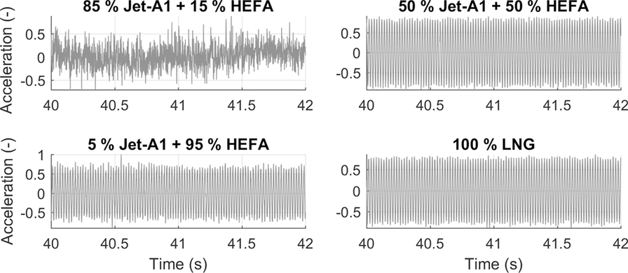
Figure 2. Normalized time-domain plots of engine vibration on four different fuel blends at the highest air-to-fuel ratio tested.

FIGURE 3

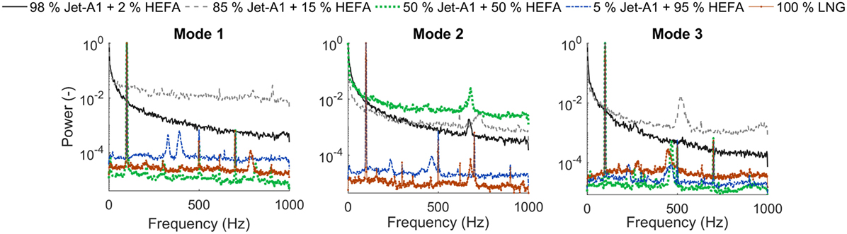
Figure 3. Normalized power spectral density plots of engine vibration on five different fuel blends from the lowest (Mode 1) to the highest (Mode 3) air-to-fuel ratio.

It is hard to provide a theoretical explanation of the physical context behind the vibration responses acquired, without a valid physics-based model that can predict the engine’s vibration response as an output of a system where, apart from the dynamics context, complex thermochemical, and other physical processes take place. At the same time, the nature of the modeling/monitoring problem, if approached from a physics-based perspective, suggests that model validation would be a significant challenge. Choosing a data-driven strategy overcomes this challenge, since the system examined (engine in operation) is treated as a black box.

Data Analysis Methods

As mentioned in the Section “INTRODUCTION,” this study follows a machine-learning framework for the condition monitoring of engines using vibration data. This means that, to develop a methodology that can be used to detect novel engine patterns from vibration data, three subsequent steps should be taken, following the data acquisition stage. Those are, namely, data preprocessing, feature extraction, and development of a learning model of normal engine behavior (Tarassenko et al., 2009).

Preprocessing of Raw Vibration Data

To improve the ability of the novelty detection scheme to determine whether a data point belongs to the class 𝒩 or 𝒜, while removing absolute values, a preprocessing method was applied prior to feature extraction. As has been shown in Clifton et al. (2006), this step has a major effect for the novelty detection system since it enables a better discriminating capability between the two different classes. Scaling and normalization is also important for most condition monitoring systems for the removal of any undesirable environmental or operational effects in the analyzed data (He et al., 2009). As a preprocessing method, it is considered for improving the performance of one-class classifiers (Juszczak et al., 2002): it is a very good practise when working with machine-learning algorithms to scale the data being analyzed, since large absolute value ranges of features will tend to dominate the ones with smaller value ranges (Hsu et al., 2016). In this study, the aim is to enhance the difference in vibration amplitude for classes 𝒩 and 𝒜, and therefore, the data are chosen to be scaled across the different conditions tested (not across time).

First, a D-dimensional matrix X = {x₁, …, x_N} of class 𝒩 was constructed. An index i = 1, …, N is used to denote the different conditions that were included in this matrix, i.e., the various fuel blends on the three modes of operation. A separate matrix Z = {z₁, …, z_L} containing data from both classes (25% of engine conditions are from class 𝒜), was also constructed. This prior labeling of the two classes, was performed by assembling a matrix with all the raw data (prior to preprocessing) and reducing its dimensions to 2 using principal component analysis (PCA), for visualizing it. The observed data points in the two-dimensional space of PCA that were far from the rest of the data were assigned the class 𝒜 label, while all the others they were given the class 𝒩 label. For instance, the condition 85% Jet-A1 + 15% HEFA at Mode 1 was given the former label.

The scaled version of matrix X was obtained as follows:

${\mathrm{\chi }}_i=\left[{\mathit{\text{x}}}_i-\overline{\mathit{\text{x}}}\right]∕{\mathrm{\sigma }}_x,$ (1)

where the mean vector is defined as $\overline{\mathit{\text{x}}}=\frac{1}{N}{\displaystyle \underset{i=1}{\sum ^N}}{\mathit{\text{x}}}_i$ and the variance vector as ${\mathrm{\sigma }}_x=\frac{1}{N}{\displaystyle \underset{i=1}{\sum ^N}}{\left({\mathit{\text{x}}}_i-\overline{\mathit{\text{x}}}\right)}^2$. Now, the scaled version of matrix Z, with an index denoting the different conditions in the matrix j = 1, …, L, containing data from both classes was obtained as follows:

${\mathrm{\zeta }}_j=\left[{\mathit{\text{z}}}_j-\overline{\mathit{\text{x}}}\right]∕{\mathrm{\sigma }}_x.$ (2)

Feature Extraction of Preprocessed Raw Vibration Data

The process of feature extraction follows after the data preprocessing stage. The wavelet packet transform (WPT) is chosen for this purpose. All the coefficients from the time-scale transformations are used as inputs to an algorithm that is suitable for linear or non-linear dimensionality reduction, the kernel principal component analysis (KPCA). This procedure of data transformation using wavelet bases and projection onto a set of lower-dimensional axes is advantageous in cases when there is no knowledge about the characteristic frequencies of the mechanical system being monitored.

Wavelet Coefficients

The objective of this stage is to obtain a set of discriminating features from the preprocessed raw vibration data, so that the learning model will then be able to easily separate the two classes of engine conditions. It was previously shown in Figure 3 that there is a certain degree of dissimilarity between the engine conditions with regards to their amplitudes in the frequency spectrum. Hence, to capture both time- and frequency-domain information from the data, it is necessary to use time–frequency methods. The wavelet transform allows one to include time information for the frequency components. Non-stationary events can, therefore, be analyzed using the wavelet transform. It is expected that the data can be more effectively described than with Fourier-based methods, where any non-stationary regions of the stochastic signal are not localized in time. Choosing a time–frequency approach, such as the wavelet transform, might be the best option for the type of data processed in this study. The simplest time–frequency analysis method, the short-time Fourier Transform, will not be an optimal option as the window size is fixed. Hence, there exist resolution limitations, determined by the uncertainty principle, which could hinder the analysis of potentially non-stationary parts of the signal.

The wavelet transform solves the problem of fixed window size, by using short windows to analyze high frequency components (good time localization) and large windows for low frequency components (good frequency localization). An example of wavelet transforms applied for condition monitoring applications was presented in Fan and Zuo (2006). Several other frequency methods exist for monitoring applications, e.g., the Empirical Mode Decomposition, as presented in Antoniadou et al. (2015), which can offer similar benefits to the wavelet transform. However, the latter method is chosen in this work because it is very easy to implement and a proven concept that is mathematically well grounded. The wavelet transform was originally developed for constructing a map of dilation and translation parameters. The dilation represents the scales s ≈ 1/frequency and translation τ refers to the time-shift operation. Consider the nth engine condition χ_n(t), with t = {0, …, 110} s. The corresponding wavelet coefficients can be calculated as follows:

$c\left(s,\mathrm{\tau }\right)=\int {\mathrm{\chi }}_n\left(t\right){\mathrm{\psi }}_{s,\mathrm{\tau }}\left(t\right)\mathit{dt}.$ (3)

The function ψ_s,τ represents a family of high frequency short time-duration and low frequency large time-duration functions of a prototype function ψ. In mathematical terms, it is defined as follows:

${\mathrm{\psi }}_{s,\mathrm{\tau }}\left(t\right)=\frac{1}{\sqrt{\left|s\right|}}\mathrm{\psi }\left(\frac{t-\mathrm{\tau }}{s}\right),s>0,$ (4)

when s < 1 the prototype function has a shorter duration in time, while when s > 1 the prototype function becomes larger in time, corresponding to high and low frequency characteristics, respectively.

In Mallat (1999), the discrete version of Eq. 3, namely, the discrete wavelet transform (DWT), was developed as an efficient alternative to the continuous wavelet transform. In particular, it was proven that using a scale j and translation k, that take only values of powers of 2, instead of intermediate ones, a satisfactory time–frequency resolution can be still obtained. This is called the dyadic grid of wavelet coefficients, and the function presented in Eq. 4, becomes a set of orthogonal wavelet functions:

${\mathrm{\psi }}_{j,k}\left(t\right)=2^{j∕2}\mathrm{\psi }\left(2^{j}t-k\right),$ (5)

such that redundancy is eliminated using this set of orthogonal wavelet bases, as described in more detail in Farrar and Worden (2012).

In practice, the DWT coefficients are obtained by convolving χ_n(t) with a set of half-band (containing half of the frequency content of the signal) low- and high-pass filters (Mallat, 1989). This yields the corresponding low- and high-pass sub-bands of the signal. Subsequently, the low-pass sub-band is further decomposed with the same scheme after decimating it by 2 (half the samples can be eliminated per Nyquist criterion), while the high-pass sub-band is not analyzed further. The signal after the first level of decomposition will have twice the frequency resolution than the original signal, since it has half the number of points. This iterative procedure is known as two-channel sub-band coding (Mallat, 1999) and provides one with an efficient way for computing the wavelet coefficients using conjugate quadrature mirror filters. Because of the poor frequency resolution of the DWT at high frequencies, the WPT was chosen for feature transformation. The difference between DWT and WPT, lies on the fact that the latter decomposes the higher-frequency sub-band further. The schematic diagram of the WPT up to 2 levels of decomposition is shown in Figure 4. First, the signal χ_n(t) is convolved with a half-band low-pass filter h(k) and a high-pass filter g(k). This gives, the wavelet coefficient vector c_1,1, which captures the lower-frequency content [0, f_s/4] Hz and the wavelet coefficient vector c_2,1 that captures the higher-frequency content (f_s/4, f_s/2) Hz. After j levels of decomposition the coefficients from the output of each filter are assembled on a matrix c_n, corresponding to the nth engine condition χ_n. Note that each coefficient has half the number of samples as χ_n(t) in the first level of decomposition. In this study, four levels of decomposition were considered as an intermediate value. The above process was repeated for the rest of the N − 1 engine conditions to get the matrix of coefficients C = {c₁, …, c_N}.

FIGURE 4

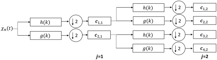
Figure 4. Wavelet packet transform schematic diagram up to decomposition level 2. At each level, the frequency spectrum is split into 2^j sub-bands.

Low-Dimensional Features

The wavelet coefficients matrix C is a D-dimensional matrix, i.e., it has the same dimensions as the original dataset. Hence, lower-dimensional features are necessary to prevent overfitting, which is associated with higher dimensions of features. In this study, the PCA, was initially used for visualization purposes, e.g., to observe possible clusters of the data points for matrix X. Its non-linear equivalent, the KPCA, is used for dimensionality reduction so that non-linear relationships between the features can be captured.

Principal component analysis is a method that can be used to obtain a new set of orthogonal axes that show the highest variance in the data. Hence, C was projected onto 2 orthogonal axes, from its original dimension D. In PCA, the eigenvalues λ_k and eigenvectors u_k of the covariance matrix S_C of C are obtained by solving the following eigenvalue problem:

${\mathit{\text{S}}}_C{\mathit{\text{u}}}_k={\mathrm{\lambda }}_k{\mathit{\text{u}}}_k,$ (6)

where k = 1, …, D. The eigenvector u₁, corresponding to the largest eigenvalue λ₁ is the first principal component, and so on. The two-dimensional representation of C, i.e., Y (an N × k matrix), can be calculated through linear projection, using the first two eigenvectors:

$\mathit{\text{Y}}=\mathit{\text{C}}{\mathit{\text{u}}}_{k=1,2}.$ (7)

In Schölkopf et al. (1998), the KPCA was introduced. This method is the generalized version of the PCA because scalar products of the covariance matrix S_C are replaced by a kernel function. In KPCA, the mapping ϕ of two data points, e.g., the nth and the mth wavelet coefficient vector c_n and c_m, respectively, is obtained with the RBF kernel function as follows:

$k\left({\mathit{\text{c}}}_n,{\mathit{\text{c}}}_m\right)=e^{\frac{{∥{\mathit{\text{c}}}_n-{\mathit{\text{c}}}_m∥}^2}{2{\mathrm{\sigma }}_{\text{KPCA}}^2}}.$ (8)

Using the above mapping, standard PCA can be performed in this new feature space ℱ, which implicitly corresponds to a non-linear principal component in the original space. Hence, the scalar products of the covariance matrix are replaced with the RBF kernel as follows:

${\mathit{\text{S}}}_{\mathrm{\varphi }}=1∕N{\displaystyle \underset{i}{\sum ^N}}\mathrm{\varphi }{\left({\mathit{\text{c}}}_{\mathit{\text{i}}}\right)}^T\mathrm{\varphi }\left({\mathit{\text{c}}}_i\right).$ (9)

However, the above matrix cannot be used directly to solve an eigenvalue problem as in Eq. 6, because of its high dimension. Hence, after some algebraic manipulation, the eigenvalues ℓ_d and eigenvectors ${\mathit{\text{u}}}_d$ can be computed for the kernel matrix 𝒦 (of size N × N), instead of the covariance matrix (of size ℱ × ℱ). Therefore, in KPCA, we are required to find a solution to the following eigenvalue problem instead:

$\mathcal{K}{\mathit{\text{u}}}_d={\ell }_d{\mathit{\text{u}}}_d,$ (10)

where d = {1, …, N}, since ℱ > N, the number of non-zero eigenvalues cannot exceed the number of engine operating conditions N (Bishop, 2006). Using the eigenvectors of the kernel matrix, it is possible to obtain the new projections $\mathcal{Y}=\left\{{\mathit{\text{y}}}_1,\dots ,{\mathit{\text{y}}}_N\right\}$ of the mapped data points of wavelet coefficients ϕ(c_i) on a non-linear surface of dimensionality d that can vary from 1 up to N.

Learning Model for Novelty Detection

Support vector machines as a tool for classification offer the flexibility of an artificial neural network, while overcoming its pitfalls. Using a kernel function to expand the original input space into a higher dimensional one to find a linear decision hyperplane is closely related to adding more layers to an artificial neural network. Therefore, the algorithm can be adapted to match the characteristics of our data better, in such a manner that enhances the prediction accuracy. Given that OCSVM forms a quadratic optimization problem, it guarantees to find the optimal solution to where the linear decision hyperplane must be positioned (Schölkopf et al., 2001; Shawe-Taylor and Cristianini, 2004). On the other hand, it is possible to obtain a local optimum as a solution to finding the mean squared error in an artificial neural network using the gradient descend algorithm.

As training data, we use the matrix obtained from KPCA, i.e., 𝒴. Whereas, lower-dimensional representations of testing data (from the matrix Z) are obtained by following the same feature transformation, selection, etc. The OCSVM methodology allows the use of the RBF kernel function, which maps the data points in 𝒴 in a similar way as that in KPCA. However, the formulation in the LIBSVM toolbox (Chang and Lin, 2011) is slightly different for the RBF kernel. Given two data points ${\mathit{\text{y}}}_n$ and ${\mathit{\text{y}}}_m$, the RBF kernel implemented in the OCSVM is defined as follows:

$k\left({\mathit{\text{y}}}_n,{\mathit{\text{y}}}_m\right)=e^{-\mathrm{\gamma }{∥{\mathit{\text{y}}}_n-{\mathit{\text{y}}}_m∥}^2}.$ (11)

After the training data are mapped via the RBF kernel, the origin in this new feature space is treated as the only member of class 𝒜 data. Then, a hyperplane is defined such that the mapped training data are separated from the origin with maximum margin. The hyperplane in the mapped feature space is located at $\mathrm{\varphi }\left({\mathit{\text{y}}}_i\right)-\mathrm{\rho }=0$, where ρ is the overall margin variable. To separate all mapped data points from the origin, the following quadratic program needs to be solved:

$\begin{array}{l}\underset{\text{w,ρ,ξ}}{\text{min}}0.5w^{T}w+\frac{1}{\upsilon N}{\displaystyle \sum _i{\text{ξ}}_i}-\text{ρ}\\ \text{subject to: (}w\mathrm{\varphi }\text{ (}{y}_i\text{))}\ge \text{ρ}-{\text{ξ}}_i,i=1,\dots ,N,{\text{ξ}}_i\ge 0,\end{array}$ (12)

where w is the normal vector to the hyperplane and ξ are called slack variables and are used to quantify the misclassification error of each data point, separately, according to the distance from its corresponding boundary. The value ν that was previously mentioned is responsible for penalizing for misclassifications and is bounded ν ∈ (0, 1]. The decision that determines whether an unseen data point ${\mathit{\text{y}}}^{\ast }$, i.e., from matrix Z, belongs to either of the two classes of engine conditions can be made by using the following function:

$g\left({\mathit{\text{y}}}^{\ast }\right)=\text{sgn}\left[\mathit{\text{w}}\mathrm{\varphi }\left({\mathit{\text{y}}}^{\ast }\right)-\mathrm{\rho }\right].$ (13)

For a data point from class 𝒜, $g\left({\mathit{\text{y}}}^{\ast }\right)>0$, otherwise, $g\left({\mathit{\text{y}}}^{\ast }\right)\le 0$. Note that for practical reasons, the optimization problem in Eq. 12 is solved by introducing Lagrange multipliers. One of the main reasons for that is because it enables the optimization to be written in terms of dot products. This gives rise to the “kernel trick,” which enables the problem to be generalized to the non-linear case by using suitable kernel functions, such as the RBF kernel that is used in this study.

Results and Discussion

In this work, the RBF kernel was used to map the data points of the OCSVM to an infinite dimensional feature space, where linear separation of the two classes can be achieved. By employing an OCSVM to our problem, we have available a wide range of kernel function formulations to use. The RBF kernel is one of the most popular ones, since it implies general smoothness properties for a dataset, an assumption that is commonly accepted in many real-world applications, as discussed in more detail in Scholkopf and Smola (2001). An RBF kernel has two parameters that need to be determined to adapt the OCSVM algorithm to the characteristics of the vibration signals expected in this study. These parameters are called the kernel width γ and optimization penalty ν. By observing the variation in validation accuracy α_ν of the OCSVM on a fine grid of values of γ and ν, it was possible to determine the combination of those two values that maximize α_ν. The values of γ and ν were chosen in steps of powers of 2, as suggested from a practical study in Hsu et al. (2016). The validation accuracy was calculated using a 10-fold cross-validation scheme to prevent overfitting the data. As discussed in more detail in Bishop (2006), the cross-validation scheme is used when the supply of training data is small. In such cases, there are not enough data to separate them into training and validation datasets, to investigate the model robustness and accuracy. In our study, the number of engine operating conditions is relatively small as compared to the number of dimensions in the feature matrix. Therefore, cross-validation scheme is a possible solution to the problem of insufficient training data. In more detail, in this scheme the data are first divided into 10 equal-sized subsets. Each subset is used to test the model’s (which was trained on the other nine subsets) classification performance sequentially. Each data point in the dataset of vibration training data is predicted once. Hence, the cross-validation accuracy is the percentage of correct classifications among the dataset of vibration training data.

In Figure 5, we present two exemplar results of cross-validation accuracies variation on a grid space of γ and ν parameters. These results correspond to the cross-validation accuracies obtained by training the OCSVM with the wavelet coefficients dataset after being “compressed” with PCA (right plot) and KPCA (left plot). The cross-validation accuracy was evaluated with ν. in the range of 0.001 and 0.8 in steps of 0.002, while γ being in the range of 2⁻²⁵ and 2²⁵ in steps of 2. The choice of this grid space for ν was made on the fact that this parameter is bounded, as it represents the upper bound of the fraction of training data that lie on the wrong side of the hyperplane [see more details in Schölkopf et al. (2001)]. In the case of γ, there was no upper and lower limits, therefore, a relatively wider range was selected. In both cases, the steps were determined such that computational costs were kept to a reasonable amount. Generally, the grid space decision followed a trial and error procedure for the given vibration dataset, to determine suitable boundaries and step size. As can be observed from the contour plots, the grid search allows us to obtain a high validation accuracy when an appropriate combination of γ and ν is chosen. For our dataset, this combination can be found mostly on relatively low values of γ. As the value of γ decreases, the pairwise distances between the training data points become less important. Therefore, the decision boundary of the OCSVM becomes more constrained, and its shape less flexible due to the fact that it will give less weight to these distances. Note that the examples in Figure 5, were produced with a d = 100 for 𝒴 and D = 100 for Y (see Low-Dimensional Features), with the decomposition level of WPT j = 4 and (for KPCA only) a kernel width γ_KPCA = 1. Clearly, using KPCA with the RBF kernel, a maximum cross-validation accuracy of around 95% can be obtained, while with the standard PCA the classification accuracy of the OCSVM is relatively poor, i.e., around 60%. Hence, there is an advantage of using KPCA over standard PCA for the specific dataset that is being used in this study. This is expected since KPCA finds non-linear relationships that exist between the data features.

FIGURE 5

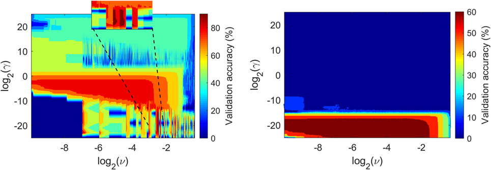
Figure 5. Cross-validation accuracy variation with γ and ν for the one-class support vector machine-based learned model using features of kernel principal component analysis (left) and standard principal component analysis.

The grid search method for finding “suitable” values for γ and ν, offers an advantage when other parameters, e.g., KCPA kernel width σ_KPCA, cannot be determined easily. It can be demonstrated that α_ν can be increased significantly, in comparison to a fixed set of default values. The LIBSVM toolbox suggests the default values to be ν = d⁻¹ and γ = 0.5. In Figure 6, the validation accuracy is shown for different values of KPCA kernel width σ_KPCA and number of principal components d, for the cases when γ and ν were selected from grid search and when they were given their fixed default values. It is clear from those two plots that the OCSVM parameters γ and ν can be “tuned” such that the validation accuracy can be maximized, regardless of the choice of d and σ_KPCA. This observation illustrates the strength of kernel-based methods, in general, since the kernel width can have a great influence in describing the training data. Most of the times, choosing this parameter is only necessary to obtain a suitable adaptation of our algorithms (Shawe-Taylor and Cristianini, 2004). As can be seen by choosing different ν and γ combinations each time (according to the grid search procedure), the maximum achievable validation accuracy is always close to 100%. This is a major improvement from the corresponding accuracy that can be obtained using the fixed set of values. Moreover, this demonstrates that it is not so challenging to “tune” a support vector machine, since there are only two parameters that need to be found, and this can be done using the grid search procedure. In contrary, an artificial neural network requires its architecture, the learning rate of gradient descent, among other parameters to be specified beforehand, which makes the problem of “tuning” the algorithm much more difficult. Nevertheless, the strongest point of a support vector machine is its ability to obtain a global optimum solution for any chosen value of γ and ν we specified, such that its generalization capability is always maximized.

FIGURE 6

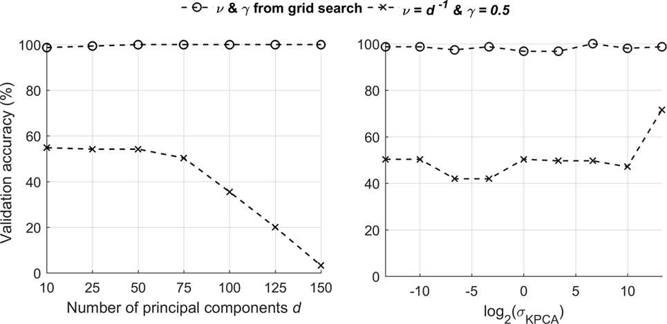
Figure 6. Variation in cross-validation accuracy for different d and σ_KPCA for selected (left) and fixed (right) γ and ν values.

As it was shown previously in Figure 5, the chosen γ value (from the grid search) was very small. This is true for every case examined, e.g., for different d values. For this reason, it can be said that the algorithm generalizes better with a less complex decision boundary. However, the “tuning” of the OCSVM proves to be challenging because the prediction accuracy (using the test data set) is lower than expected, i.e., less than 50%. Most of the errors occurred for data points wrongly accepted as coming from class 𝒜, whereas in reality they belonged to class 𝒩. Plausible reasons for the unsatisfactory performance of the OCSVM on the test data set are discussed below:

• The validation stage of the OCSVM evaluates only the errors of wrongly rejecting data from class 𝒩. One could assume that the reason behind this misclassification could be associated with the errors in the calculation of the parameters γ and ν estimated with the grid search. In terms of choosing γ and ν, there have been a few attempts to tackle this problem in different ways than grid search. For instance, in Xiao et al. (2015), the authors presented methods to choose the kernel width γ of the OCSVM with what they refer to as “geometrical” calculations.

• Due to the nature of the data, there is a lot of variability between the engine conditions and within each condition, too. Therefore, it is difficult to develop a model using class 𝒩 data if the characteristics of each condition within the same class are different. The choice of appropriate training data is an important factor for the data-driven approaches followed. In this case, the representation of the data should be chosen to be in domains with appropriate time resolution and the pattern recognition algorithms chosen should potentially not depend on training but work in an adaptive framework.

Conclusion

In this study, we have followed a novelty detection scheme for condition monitoring of engines using advanced machine-learning methods, chosen as appropriate for the kind of data analyzed. This resulted in a better description of the main challenges that can be faced when following a data-driven strategy for monitoring engine vibration data. The novelty detection scheme was chosen over a classification approach due to the lack of training data for the various states of an engine’s operation, commonly faced in real life applications. The following steps were examined as fundamental, optimal methods for the analysis of the data. A model of normality, based on OCSVMs, that was trained to recognize scenarios of normal and novel engine conditions, was developed using data from the engine operating under conditions in which the engine experienced low vibration amplitudes. The choice of this novelty detection machine-learning method was due to the fact that the pattern recognition problem is based on building a kernel that offers a versatility that can support the analysis of more complex data. In this case, according to the analysis presented in the study, the heavy influence of the penalizing parameter ν and kernel width γ of the OCSVM can affect the validation accuracy. Using a fine grid search for selecting the parameters ν and γ, it is possible to achieve close to 100% in validation accuracy, as demonstrated in the results. This is a significant advantage when there is no methodology in place in selecting other parameters, such as the number of principal components used in KPCA. This also outlines one of the strengths of kernel-based methods, which is the adaptability to a given a data set. In particular, the RBF kernel was proven very effective in describing the data from the engine, by choosing an appropriate value of its kernel width γ.

The limitations of the novelty detection approaches in general and the one discussed in particular in this study include the following points: the training vibration data that can be obtained from engines and the limitations of the specific algorithms examined. For the latter, the selection of ν and γ was discussed and an independent test data set that included 25% of conditions from novel engine behavior was used to calculate classification accuracies using the selected ν and γ from the grid search. Even though, validation results were exceptionally good and the model did not seem to overfit the data as the decision boundary was smooth and the number of support vectors relatively small, the classification accuracy using the test data set was unsatisfactory. The largest errors occurred when incorrectly predicting data points from the healthy engine conditions, as being novel. A few possible reasons as to why this can happen were mentioned in the previous part of the study.

To improve the novelty detection scheme presented in this study, some further work is required to train the OCSVM appropriately. For instance, instead of selecting ν and γ using a grid search approach, it is possible to use methods that calculate those parameters in a more principled way using simple geometry. Also, the wavelet transform features extracted from the data, might have resulted in a large scattering of data points in the feature space due to the fact that there is a high variability in the signals from each engine condition. One way to solve this problem is to examine new set of features needs that can provide better clustering of the data points from the healthy engine conditions, so that a smaller and tighter decision boundary can be formed in the feature space. Another suggestion would be the development of new machine-learning algorithms that do not rely on the quality of the training data but can rather adaptively classify the different states/operation condition of the engine examined.

Author Contributions

IM conducted the machine-learning analysis and is the first author of the study. IA supervised the work (conception and review). BK facilitated the conduction of the experiments and the acquisition of the data analyzed. All the authors are accountable for the content of the work.

Conflict of Interest Statement

The authors declare that the research was conducted in the absence of any commercial or financial relationships that could be construed as a potential conflict of interest.

Acknowledgments

The authors would like to thank the people from the Low Carbon Combustion Center at The University of Sheffield for conducting the gas turbine engine experiments and for kindly providing the engine vibration data used in this study.

Funding

IM is a PhD student funded by a scholarship from the Department of Mechanical Engineering at The University of Sheffield. All the authors gratefully acknowledge funding received from the Engineering and Physical Sciences Research Council (EPSRC) grant EP/N018427/1.

References

Antoniadou, I., Manson, G., Staszewski, W. J., Barszcz, T., Worden, K. (2015). A time–frequency analysis approach for condition monitoring of a wind turbine gearbox under varying load conditions. Mech. Syst. Signal Process. 64, 188–216. doi: 10.1016/j.ymssp.2015.03.003

CrossRef Full Text | Google Scholar

Bishop, C. (2006). Pattern Recognition and Machine Learning (Information Science and Statistics). New York: Springer.

Google Scholar

Blakey, S., Rye, L., and Wilson, W. (2011). Aviation gas turbine alternative fuels: a review. Proc. Combus. Inst. 33, 2863–2885. doi:10.1016/j.proci.2010.09.011

CrossRef Full Text | Google Scholar

Chang, C., and Lin, C. (2011). LIBSVM: a library for support vector machines. ACM Trans. Intell. Syst. Technol. 2, 1–27. doi:10.1145/1961189.1961199

CrossRef Full Text | Google Scholar

Clifton, D. A., Bannister, P. R., and Tarassenko, L. (2006). “Application of an intuitive novelty metric for jet engine condition monitoring,” in Advances in Applied Artificial Intelligence, eds M. Ali and R. Dapoigny (Berlin, Heidelberg: Springer), 1149–1158.

Google Scholar

Clifton, L., Clifton, D. A., Zhang, Y., Watkinson, P., Tarassenko, L., Yin, H. (2014). Probabilistic novelty detection with support vector machines. IEEE Trans. Reliab. 455–467. doi:10.1109/TR.2014.2315911

CrossRef Full Text | Google Scholar

Clifton, L., Yin, H., Clifton, D., and Zhang, Y. (2007). “Combined support vector novelty detection for multi-channel combustion data,” in IEEE International Conference on Networking, Sensing and Control, London.

Google Scholar

Fan, X., and Zuo, M. (2006). Gearbox fault detection using Hilbert and wavelet packet transform. Mech. Syst. Signal Process. 20, 966–982. doi:10.1016/j.ymssp.2005.08.032

CrossRef Full Text | Google Scholar

Farrar, C., and Worden, K. (2012). Structural Health Monitoring: A Machine Learning Perspective. Chichester: John Wiley & Sons.

Google Scholar

Hayton, P., Schölkopf, B., Tarassenko, L., and Anuzis, P. (2000). “Support vector novelty detection applied to jet engine vibration spectra,” in Annual Conference on Neural Information Processing Systems (NIPS), Denver.

Google Scholar

He, Q., Yan, R., Kong, F., and Du, R. (2009). Machine condition monitoring using principal component representation. Mech. Syst. Signal Process. 23, 446–466. doi:10.1016/j.ymssp.2008.03.010

CrossRef Full Text | Google Scholar

Hsu, C., Chang, C., and Lin, C. (2016). A Practical Guide to Support Vector Classification. Taipei: Department of Computer Science, National Taiwan University.

Google Scholar

Juszczak, P., Tax, D., and Duin, R. P. W. (2002). “Feature scaling in support vector data description,” in Proc. ASCI, Lochem.

Google Scholar

King, S., Bannister, P. R., Clifton, D. A., and Tarassenko, L. (2009). Probabilistic approach to the condition monitoring of aerospace engines. Proc. Inst. Mech. Eng. G J. Aerosp. Eng. 223, 533–541. doi:10.1243/09544100JAERO414

CrossRef Full Text | Google Scholar

Mallat, S. (1989). A theory of multiresolution signal decomposition: the wavelet representation. IEEE Trans. Pattern Anal. Mach. Intell. 11, 674–693. doi:10.1109/34.192463

CrossRef Full Text | Google Scholar

Mallat, S. (1999). A Wavelet Tour of Signal Processing (Wavelet Analysis and Its Applications). New York: Academic Press.

Google Scholar

Pimentel, M., Clifton, D., Clifton, L., and Tarassenko, L. (2014). A review of novelty detection. Signal Processing 99, 215–249. doi:10.1016/j.sigpro.2013.12.026

CrossRef Full Text | Google Scholar

Schölkopf, B., Platt, J. C., Shawe-Taylor, J., Smola, A. J., and Williamson, R. C. (2001). Estimating the support of a high-dimensional distribution. Neural Comput. 10, 1443–1471. doi:10.1162/089976601750264965

PubMed Abstract | CrossRef Full Text | Google Scholar

Scholkopf, B., and Smola, A. (2001). Learning with Kernels: Support Vector Machines, Regularization, Optimization, and Beyond. Cambridge: MIT Press.

Google Scholar

Schölkopf, B., Smola, A., and Müller, K. (1998). Nonlinear component analysis as a Kernel Eigenvalue Problem. Neural Comput. 10, 1299–1319. doi:10.1162/089976698300017467

CrossRef Full Text | Google Scholar

Shawe-Taylor, J., and Cristianini, N. (2004). Kernel Methods for Pattern Analysis. New York: Cambridge University Press.

Google Scholar

Tarassenko, L., Clifton, D. A., Bannister, P. R., King, S., King, D. (2009). “Chapter 35 – novelty detection,” in Encyclopedia of Structural Health Monitoring, eds C. Boller, F. Chang, and Y. Fujino (Barcelona: John Wiley & Sons).

Google Scholar

Xiao, Y., Wang, H., and Xu, W. (2015). Parameter selection of Gaussian Kernel for one-class SVM. IEEE Trans. Cybern. 45, 927–939. doi:10.1109/TCYB.2014.2340433

PubMed Abstract | CrossRef Full Text | Google Scholar