Frequency-Domain Physical-Parameter System Identification of Building Structures with Stiffness Eccentricity

Introduction

An innovative method is proposed for frequency-domain physical-parameter system identification (SI) of three-dimensional (3D) building structures with stiffness eccentricity, which accompany torsional vibration. The one-directional story stiffnesses and damping coefficients in the 3D building structure are identified from the recorded data on floor horizontal accelerations and rotational accelerations around a vertical axis. To the best of the authors’ knowledge, investigations on physical SI of 3D building structures with stiffness or mass eccentricities are quite limited. One of such examples is the paper by Omrani et al. (2012) in which many parameters to be identified in 3D building structures appear to cause difficulties. They conducted the statistical analysis and the magnitude of eccentricity was assumed a priori. On the other hand, the identification method proposed in this paper has an advantage such that the stiffness eccentricities are identified together with all stiffness and damping parameters.

Recently, the business continuity plan (BCP) is becoming a leading subject in the world and is being discussed with great concern in the construction and operating process of various built environments. Unprecedented hazards and incidents in the last few decades enhanced BCP to a key subject and many significant efforts on BCP have been devoted to assure the resilience of built environments. The structural health monitoring (SHM) plays a critical role in the development of BCP.

Structural health monitoring is of multidisciplinary nature and has a broad impact in civil, mechanical, ocean, and aerospace engineering. The recent development can be found in Boller et al. (2009) and Takewaki et al. (2011). The SI methodologies, categorized as methods for inverse problems, play a key role in SHM. The modal SI and physical SI are two major well-known branches. Originally, the modal SI as a popular technique was developed extensively. It can provide the overall mechanical properties of a structural system and has a stable characteristic (Hart and Yao, 1977, Agbabian et al., 1991, Nagarajaiah and Basu, 2009). On the other hand, the physical SI has another advantage that the stiffness and/or damping coefficients of the structural model can be recovered directly and is well suited to the design of passive control systems. This is also quite useful for the damage detection. Nevertheless that the physical SI is preferred in SHM, its development is quite limited and slow due to the strict requirement on multiple measurements or the necessity of complicated mathematical manipulation (Hart and Yao, 1977; Udwadia et al., 1978; Shinozuka and Ghanem, 1995; Takewaki and Nakamura, 2000, 2005; Brownjohn, 2003; Nagarajaiah and Basu, 2009; Takewaki et al., 2011; Zhang and Johnson, 2013; Johnson and Wojtkiewicz, 2014; Wojtkiewicz and Johnson, 2014).

In the physical SI, Nakamura and Yasui (1999) proposed a method of direct SI incorporating a least-squares method. They investigated an issue of damage detection for steel building frames, which were severely damaged (beam-end fracture, etc.) during the Hyogoken-Nanbu (Kobe) earthquake in 1995. Since their approach needs many measurement points and vibration components due to the direct use of equations of motion, it was restricted to simple shear-type building models with a small number of vibration components. Moreover, the method of Takewaki and Nakamura (2000) aims at a smart identification and seeks for a unique physical-parameter SI formulation based on the work by Udwadia et al. (1978). Takewaki and Nakamura (2000) overcame the difficulty in the method by Udwadia et al. (1978) and enabled the identification of stiffness and damping at a given story of a shear building model (S model) directly from the floor acceleration records just above and below the target story. They defined and used the so-called identification function in which the limit manipulation toward zero frequency is necessary for the identification of stiffness and damping. In the SI method by Takewaki and Nakamura (2000, 2005, 2010), there remained an issue to be resolved in dealing with actual data, e.g., micro-tremors, due to the small signal/noise (SN) ratio in the low frequency range (Ikeda et al., 2014, 2015; Fujita et al., 2015). Furthermore, an S model should be replaced by a more appropriate model when dealing with high-rise buildings with large aspect ratios due to the influence of overall bending deformation of tall buildings. The former problem has been a critical and most difficult problem in the field of the physical SI where the limit manipulation is needed in the transfer function for ω → 0. An extended ARX (Auto-Regressive with eXogenous) model with constraints on the ARX parameters has been devised by Maeda et al. (2011), Kuwabara et al. (2013), and Minami et al. (2013) to respond to the difficulty caused by the noise. By applying the extended ARX model to the abovementioned transfer functions, the difficulty encountered in the limit manipulation for data with a small SN ratio has been successfully avoided. On the other hand, the latter problem has been tackled by expanding the SI algorithm to the shear-bending model (SB model) (Fujita et al., 2013; Minami et al., 2013).

For developing a hybrid method of the modal and physical SIs, a limited number of researchers proposed a reliable method of SI, in which the physical parameters are identified from the pre-identified modal parameters (Hjelmstad et al., 1995; Fujita et al., 2017). However, it was made clear that the hybrid method needs detailed and profound understanding of the relation between the physical parameters and the modal parameters in addition to the deeper theoretical investigation on inverse problem formulation (Hjelmstad, 1996).

An SI method incorporating the Kalman filter or extended Kalman filter was developed many years ago as another effective approach (Hoshiya and Saito, 1984). Although the approach has a general mathematical framework and can deal with noise issues in an appropriate unified manner, knowledge based on strong mathematical backgrounds is required and its simple use may be difficult. Recently, an approach to the SI based on the Bayesian updating is of great concern and is developing very fast (Boller et al., 2009). The application of this approach to actual problems is of urgent priority for development and is strongly desired.

Rather recently, Shintani et al. (2017) proposed a method of physical SI for 3D building structures with in-plane rigid floor diaphragm in which the stiffness and damping coefficients of each vertical structural frame in the 3D building structure are recovered from the measured data on floor horizontal accelerations. A method based on the batch processing least-squares estimation was proposed using many discrete time-domain data to directly identify the stiffness and damping coefficients of each vertical structural frame. While previous researches on SI of 3D building structures are limited to a class of structures with regular eccentricity, the paper by Shintani et al. (2017) removed this limitation and opened a door for general identification of 3D building structures with general properties. Their method does not need to give the stiffness eccentricities (location of center of stiffness) before identification and the stiffness and damping parameter identification can be performed simultaneously. However, their method has a difficulty that all the displacements, velocities, and accelerations have to be provided.

A method of frequency-domain physical SI is developed here for 3D building structures with stiffness eccentricity. Equations of motion in the time domain are transformed into the frequency domain. In addition to the identification of stiffness and damping coefficients, the quantities of stiffness eccentricities in all stories can be identified using the slopes of the functions for identification of torsional stiffness in the frequency domain. The reliability and accuracy of the proposed method are demonstrated by numerical simulations and scaled experiments.

Identification Algorithm

Object Building Model and Assumptions

Consider an N-story 3D building model, with stiffness symmetricity with respect to the x-axis, as shown in Figure 1. L_x, L_y denote the x-directional and y-directional floor sizes as shown in Figure 1. The building model is subjected to the earthquake ground motion input in the y-direction and exhibits a torsional response. Let m_j, I_j, k_yj, k_θj, e_xj denote the j-th story mass, the j-th story mass moment of inertia, the story stiffness of the j-th story, the torsional stiffness of the j-th story around the center of mass, and the eccentricity of the center of stiffness from the center of mass in the j-th story, respectively. The frame in the side of the center of stiffness is called the stiff-side frame and the frame in the other side of the center of stiffness is called the flexible-side frame.

FIGURE 1

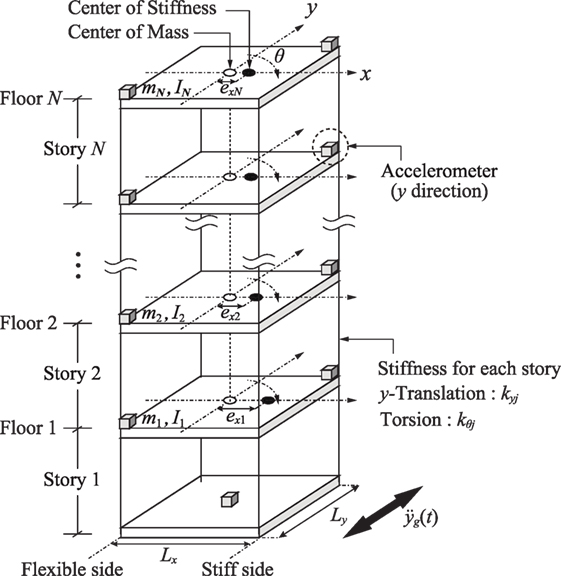
Figure 1. Three-dimensional multi-story building structure model with stiffness eccentricity subjected to unidirectional earthquake ground motion and allocation of accelerometers.

The following assumptions on the building model are introduced.

(1) The center of mass in each story exists in the common vertical line.

(2) The building model is linearly elastic and has a stiffness-proportional damping matrix.

(3) The building model has the stiffness symmetricity with respect to the x-axis (the center of stiffness exists on the x-axis) and exhibits a torsional response under the y-directional input.

(4) The floor is rigid in its in-plane deformation and the building model can be expressed by a three-dimensional shear building model with y-directional vibration eccentricity (i.e., the center of stiffness exists on the x-axis except the center of mass).

In the identification, the following two conditions are used.

(1) The floor masses {m_j}, the mass moment of inertia {I_j}, and the location of the common center of mass are known.

(2) The y-directional accelerations at the stiff-side and the flexible-side of all the floors and that on the ground floor are measured.

Formulation of Identification Theory

The equations of motion of this building model subjected to the earthquake ground acceleration ${ÿ}_g\left(t\right)$ in the y-direction may be expressed by

$\mathbf{\text{M}}\ddot{{u}}\left(t\right)+\mathbf{\text{C}}\dot{{u}}\left(t\right)+\mathbf{\text{K}}{u}\left(t\right)=-\mathbf{\text{Mr}}{ÿ}_g\left(t\right),$ (1)

where the mass, stiffness, and damping matrices M, K, C, the displacement vector u(t) [y-directional displacements y(t) of the center of mass and floor rotation angles θ(t)] and the influence coefficient vector r may be given as follows.

(2a-e)$\begin{array}{l}\mathbf{\text{M}}=\left[\begin{array}{cc}\hfill \mathbf{\text{m}}\hfill & \hfill \mathbf{\text{0}}\hfill \\ \hfill \mathbf{\text{0}}\hfill & \hfill \mathbf{\text{I}}\hfill \end{array}\right],\mathbf{\text{K}}=\left[\begin{array}{cc}\hfill {\mathbf{\text{K}}}_{\mathit{yy}}\hfill & \hfill {\mathbf{\text{K}}}_{y\mathrm{\theta }}\hfill \\ \hfill {\mathbf{\text{K}}}_{\mathrm{\theta }y}\hfill & \hfill {\mathbf{\text{K}}}_{\mathrm{\theta }\theta }\hfill \end{array}\right],\mathbf{\text{C}}=\frac{2h_1}{{\mathrm{\omega }}_1}\mathbf{\text{K}},\\ \mathbf{\text{u}}\left(t\right)=\left\{\begin{array}{c}\hfill \mathbf{\text{y}}\left(t\right)\hfill \\ \hfill \mathrm{\theta }\left(t\right)\hfill \end{array}\right\},\mathbf{\text{r}}=\left\{\begin{array}{c}\hfill \mathbf{\text{1}}\hfill \\ \hfill \mathbf{\text{0}}\hfill \end{array}\right\},\end{array}$

ω₁ and h₁ denote the fundamental natural circular frequency and the lowest-mode damping ratio. Other parameters may be defined as follows.

(3a-h)$\begin{array}{l}\mathbf{\text{m}}=\text{diag\hspace{0.17em}}\left\{m_1\text{,}{m}_2\text{,}\dots \text{,}{m}_N\right\},\\ \mathbf{\text{I}}=\text{diag\hspace{0.17em}}\left\{I_1\text{,}{I}_2\text{,}\dots \text{,}{I}_N\right\},\\ \mathbf{\text{y}}\left(t\right)\text{=}\left\{y_1\right(t\text{),}{y}_2(t\text{),}\dots \text{,}{y}_N(t){\}}^{\mathit{\text{T}}},\\ \mathrm{\theta }\left(t\right)\text{=}\{{\mathrm{\theta }}_1\left(t\text{),}{\mathrm{\theta }}_2\right(t\text{),}\dots \text{,}{\mathrm{\theta }}_N\left(t\right){\}}^{\mathit{\text{T}}},\\ \mathbf{\text{1}}={\left\{1,1,\dots ,1\right\}}^T,\\ {\mathbf{\text{K}}}_{\mathit{yy}}=\left[\begin{array}{cccc}\hfill k_{y1}+k_{y2}\hfill & \hfill -k_{y2}\hfill & \hfill \cdots \hfill & \hfill 0\hfill \\ \hfill -k_{y2}\hfill & \hfill k_{y2}+k_{y3}\hfill & \hfill \hfill & \hfill ⋮\hfill \\ \hfill ⋮\hfill & \hfill \hfill & \hfill \ddots \hfill & \hfill -k_{\mathit{yN}}\hfill \\ \hfill 0\hfill & \hfill \cdots \hfill & \hfill -k_{\mathit{yN}}\hfill & \hfill k_{\mathit{yN}}\hfill \end{array}\right],\\ {\mathbf{\text{K}}}_{\theta \mathrm{\theta }}=\left[\begin{array}{cccc}\hfill k_{\theta 1}+k_{\theta 2}\hfill & \hfill -k_{\theta 2}\hfill & \hfill \cdots \hfill & \hfill 0\hfill \\ \hfill -k_{\theta 2}\hfill & \hfill k_{\theta 2}+k_{\theta 3}\hfill & \hfill \hfill & \hfill ⋮\hfill \\ \hfill ⋮\hfill & \hfill \hfill & \hfill \ddots \hfill & \hfill -k_{\mathrm{\theta }N}\hfill \\ \hfill 0\hfill & \hfill \cdots \hfill & \hfill -k_{\mathrm{\theta }N}\hfill & \hfill k_{\mathrm{\theta }N}\hfill \end{array}\right],\\ {\mathbf{\text{K}}}_{y\mathrm{\theta }}={\mathbf{\text{K}}}_{\mathrm{\theta }y}^T=\left[\begin{array}{cccc}\hfill -\left(k_{y1}{e}_{x1}+k_{y2}{e}_{x2}\right)\hfill & \hfill k_{y2}{e}_{x2}\hfill & \hfill \cdots \hfill & \hfill 0\hfill \\ \hfill k_{y2}{e}_{x2}\hfill & \hfill -\left(k_{y2}{e}_{x2}+k_{y3}{e}_{x3}\right)\hfill & \hfill \hfill & \hfill ⋮\hfill \\ \hfill ⋮\hfill & \hfill \hfill & \hfill \ddots \hfill & \hfill k_{\mathit{yN}}{e}_{\mathit{xN}}\hfill \\ \hfill 0\hfill & \hfill \cdots \hfill & \hfill k_{\mathit{yN}}{e}_{\mathit{xN}}\hfill & \hfill -k_{\mathit{yN}}{e}_{\mathit{xN}}\hfill \end{array}\right],\end{array}$

The Fourier transformation of Eq. 1 leads to the following equations of motion in the frequency domain.

$\left(-{\mathrm{\omega }}^2\mathbf{\text{M}}+i\mathrm{\omega }\mathbf{\text{C}}+\mathbf{\text{K}}\right)\mathbf{\text{U}}\left(\mathrm{\omega }\right)=-\mathbf{\text{Mr}}{\ddot{Y}}_g\left(\mathrm{\omega }\right),$ (4)

where $\mathbf{\text{U}}\left(\mathrm{\omega }\right)={\left\{\mathbf{\text{Y}}{\left(\mathrm{\omega }\right)}^{\mathit{\text{T}}}\mathrm{\Theta }{\left(\mathrm{\omega }\right)}^{\mathit{\text{T}}}\right\}}^{\mathit{\text{T}}}$ and ${\ddot{Y}}_g\left(\mathrm{\omega }\right)$ are the Fourier transforms of u(t) and ${ÿ}_g\left(t\right)$. The capital letters indicate the Fourier transforms of variables in the time domain in the following. Eq. 4 can also be expressed as

$\left(-{\mathrm{\omega }}^2\mathbf{\text{M}}+i\mathrm{\omega }\mathbf{\text{C}}+\mathbf{\text{K}}\right)\ddot{\mathbf{\text{U}}}\left(\mathrm{\omega }\right)={\mathrm{\omega }}^2\mathbf{\text{Mr}}{\ddot{Y}}_g\left(\mathrm{\omega }\right).$ (5)

The capital letters indicate the Fourier transforms of responses later.

The y-directional equilibrium of the free-body above the j-th story may be expressed in the frequency domain by

$\begin{array}{l}\begin{array}{ll}{\mathrm{\omega }}^2{\displaystyle \underset{k=j}{\sum ^N}}{m}_k\left({\ddot{Y}}_k+{\ddot{Y}}_g\right)& =\left(k_{\mathit{yj}}+i\mathrm{\omega }\frac{2h_1}{{\mathrm{\omega }}_1}{k}_{\mathit{yj}}\right)\times \left\{\left({\ddot{Y}}_j-{\ddot{Y}}_{j-1}\right)-e_{\mathit{xj}}\left({\ddot{\mathrm{\Theta }}}_j-{\ddot{\mathrm{\Theta }}}_{j-1}\right)\right\}\hfill \\ \hfill & =\left(k_{\mathit{yj}}+i\mathrm{\omega }{c}_{\mathit{yj}}\right)\times \left\{\left({\ddot{Y}}_j-{\ddot{Y}}_{j-1}\right)-e_{\mathit{xj}}\left({\mathrm{\Theta }}_j-{\ddot{\mathrm{\Theta }}}_{j-1}\right)\right\},\end{array}\hfill \end{array}$ (6)

where ${\ddot{Y}}_0=0$, ${\ddot{\mathrm{\Theta }}}_0=0$ and the viscous damping coefficient c_yj in the j-th story is given by

$c_{\mathit{yj}}=\frac{2h_1}{{\mathrm{\omega }}_1}{k}_{\mathit{yj}}.$ (7)

Rearrangement of Eq. 6 with respect to k_yj and c_yj yields

$\begin{array}{ll}\hfill k_{\mathit{yj}}+i\mathrm{\omega }{c}_{\mathit{yj}}& =\frac{{\mathrm{\omega }}^2{\displaystyle \sum _{k=j}^N}{m}_k\left({\ddot{Y}}_k+{\ddot{Y}}_g\right)}{\left({\ddot{Y}}_j-{\ddot{Y}}_{j-1}\right)-e_{\mathit{xj}}\left({\ddot{\mathrm{\Theta }}}_j-{\ddot{\mathrm{\Theta }}}_{j-1}\right)}\\ & =\frac{{\mathrm{\omega }}^2{\displaystyle \sum _{k=j}^N}{m}_k{\ddot{Y}}_k^{\text{abs}}}{\left({\ddot{Y}}_j^{\text{abs}}-{\ddot{Y}}_{j-1}^{\text{abs}}\right)-e_{\mathit{xj}}\left({\ddot{\mathrm{\Theta }}}_j-{\ddot{\mathrm{\Theta }}}_{j-1}\right)},\end{array}$ (8)

where ${\ddot{Y}}_j^{\text{abs}}$ indicates the Fourier transform of the absolute acceleration at the center of mass in the j-th floor and ${\ddot{Y}}_0^{\text{abs}}={\ddot{Y}}_g$.

Since the y-directional accelerations at the stiff-side and the flexible-side of all the floors are measured, it is tried to express the absolute acceleration at the center of mass in terms of the accelerations at the stiff-side and the flexible-side. If the location parameter of the center of mass is denoted by α (given parameter/dividing ratio), the absolute acceleration ${\ddot{Y}}_j^{\text{abs}}$ at the center of mass can be expressed by

${\ddot{Y}}_j^{\text{abs}}=\mathrm{\alpha }{\ddot{Y}}_{j,F}^{\text{abs}}+\left(1-\mathrm{\alpha }\right){\ddot{Y}}_{j,S}^{\text{abs}},$ (9)

where ${\ddot{Y}}_{j,F}^{\text{abs}}$ and ${\ddot{Y}}_{j,S}^{\text{abs}}$ denote the Fourier transform of the y-directional absolute accelerations at the flexible-side and the stiff-side in the j-th story, respectively. The denominator of Eq. 8 indicates the inter-story quantity of absolute accelerations at the center of stiffness and is expressed by

$\begin{array}{l}\hfill \left({\ddot{Y}}_j^{\text{abs}}-{\ddot{Y}}_{j-1}^{\text{abs}}\right)-e_{\mathit{xj}}\left({\ddot{\mathrm{\Theta }}}_j-{\ddot{\mathrm{\Theta }}}_{j-1}\right)={\mathrm{\beta }}_j\left({\ddot{Y}}_{j,F}^{\text{abs}}-{\ddot{Y}}_{j-1,F}^{\text{abs}}\right)+\left(1-{\mathrm{\beta }}_j\right)\left({\ddot{Y}}_{j,S}^{\text{abs}}-{\ddot{Y}}_{j-1,S}^{\text{abs}}\right),\end{array}$ (10)

where β_j is a parameter for defining the location of the center of stiffness and is given by

${\mathrm{\beta }}_j=\mathrm{\alpha }-\frac{e_{\mathit{xj}}}{L_x}={\mathrm{\beta }}_j\left(e_{\mathit{xj}}\right).$ (11)

Substitution of Eqs 9 and 10 into Eq. 8 provides

$\begin{array}{ll}\hfill k_{\mathit{yj}}+i\mathrm{\omega }{c}_{\mathit{yj}}& =\frac{{\mathrm{\omega }}^2{\displaystyle \sum _{k=j}^N}{m}_k\left\{\mathrm{\alpha }{\ddot{Y}}_{k,F}^{\text{abs}}+\left(1-\mathrm{\alpha }\right){\ddot{Y}}_{k,S}^{\text{abs}}\right\}}{{\mathrm{\beta }}_j\left({\ddot{Y}}_{j,F}^{\text{abs}}-{\ddot{Y}}_{j-1,F}^{\text{abs}}\right)+\left(1-{\mathrm{\beta }}_j\right)\left({\ddot{Y}}_{j,S}^{\text{abs}}-{\ddot{Y}}_{j-1,S}^{\text{abs}}\right)}\\ & =f_y\left(\mathrm{\omega },{\mathrm{\beta }}_j\left(e_{\mathit{xj}}\right)\right),\end{array}$ (12)

where ${\ddot{Y}}_{0,F}^{\text{abs}}={\ddot{Y}}_{0,S}^{\text{abs}}={\ddot{Y}}_g$. This function will be called “the lateral identification function” and used for identification of k_yj.

On the other hand, the rotational equilibrium of the free-body above the j-th story leads to the function in terms of k_θj and c_θj.

$\begin{array}{l}\hfill \begin{array}{rl}{k}_{\mathrm{\theta }j}+i\mathrm{\omega }{c}_{\mathrm{\theta }j}& =\frac{{\mathrm{\omega }}^2{\displaystyle \sum _{k=j}^N}{I}_k{\ddot{\mathrm{\Theta }}}_k}{{\ddot{\mathrm{\Theta }}}_j-{\ddot{\mathrm{\Theta }}}_{j-1}}+f_y\left(\mathrm{\omega },{\mathrm{\beta }}_j\left(e_{\mathit{xj}}\right)\right)e_{\mathit{xj}}\frac{{\ddot{Y}}_j^{\text{abs}}-{\ddot{Y}}_{j-1}^{\text{abs}}}{{\ddot{\mathrm{\Theta }}}_j-{\ddot{\mathrm{\Theta }}}_{j-1}}\\ & =\frac{{\mathrm{\omega }}^2{\displaystyle \sum _{k=j}^N}{I}_k\left({\ddot{Y}}_{k,F}^{\text{abs}}-{\ddot{Y}}_{k,S}^{\text{abs}}\right)}{\left({\ddot{Y}}_{j,F}^{\text{abs}}-{\ddot{Y}}_{j,S}^{\text{abs}}\right)-\left({\ddot{Y}}_{j-1,F}^{\text{abs}}-{\ddot{Y}}_{j-1,S}^{\text{abs}}\right)}\\ & +f_y\left(\mathrm{\omega },{\mathrm{\beta }}_j\left(e_{\mathit{xj}}\right)\right)\left(\mathrm{\alpha }-{\mathrm{\beta }}_j\right)L_x^2\times \frac{\left\{\mathrm{\alpha }{\ddot{Y}}_{j,F}^{\text{abs}}+\left(1-\mathrm{\alpha }\right){\ddot{Y}}_{j,S}^{\text{abs}}\right\}-\left\{\mathrm{\alpha }{\ddot{Y}}_{j-1,F}^{\text{abs}}+\left(1-\mathrm{\alpha }\right){\ddot{Y}}_{j-1,S}^{\text{abs}}\right\}}{\left({\ddot{Y}}_{j,F}^{\text{abs}}-{\ddot{Y}}_{j,S}^{\text{abs}}\right)-\left({\ddot{Y}}_{j-1,F}^{\text{abs}}-{\ddot{Y}}_{j-1,S}^{\text{abs}}\right)}\\ & =f_{\mathrm{\theta }}\left(\mathrm{\omega },{\mathrm{\beta }}_j\left(e_{\mathit{xj}}\right)\right).\end{array}\end{array}$ (13)

In Eq. 13, the following relations are used.

$\begin{array}{ll}\hfill c_{\mathrm{\theta }j}& =\frac{2h_1}{{\mathrm{\omega }}_1}{k}_{\mathrm{\theta }j},\end{array}$ (14a)

$\begin{array}{ll}\hfill {\ddot{\mathrm{\Theta }}}_j& =\frac{{\ddot{Y}}_{j,F}^{\text{abs}}-{\ddot{Y}}_{j,S}^{\text{abs}}}{L_x}.\end{array}$ (14b)

Equation 13 will be called “the torsional identification function” and used for identification of the distance of eccentricity e_xj.

Identification of Distance between Center of Mass and Center of Stiffness

Equations 12 and 13 mean that, if the true distance of eccentricity (between the center of mass and the center of stiffness) is given, the real part and the imaginary part of the identification functions become constant with respect to frequency. On the contrary, if an erroneous distance of eccentricity is used, those functions are not constant. This property may be able to be used for the identification of the distance of eccentricity. In this paper, Eq. 13 is used because the torsional stiffness is sensitive to the variation of the distance of eccentricity compared to the lateral stiffness.

Identification of Lateral Stiffness

It is assumed that the distance of eccentricity has been identified in Section “Identification of distance between center of mass and center of stiffness.” The identification algorithm of the lateral stiffness can be summarized as follows.

(Step 1) Focusing on the fundamental natural circular frequency with high S/N ratio, pick up M data points from the identification result.

(Step 2) Classify M data points into the classes that have a particular range of values and compute the mean value from data points that lie in the class of the highest frequency.

(Step 3) Compute the coefficient of variation by using the mean value.

(Step 4) Vary the sample number M and repeat Steps 1–3.

(Step 5) Find the value corresponding to the smallest coefficient of variation and regard this as the identified value.

The detailed explanation of Steps 1–2 can be found in Figure 2. The number of classes can be defined from the Sturges’ rule by

$\text{Number of classes =}1+{\log }_{2}M.$ (15)

FIGURE 2

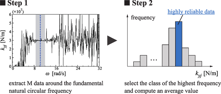
Figure 2. Identification procedure in frequency domain (Steps 1–2).

The range width per class (upper and lower limits of each class) can also be determined by using the number of classes.

Verification of Accuracy of the Proposed Method Using Numerical Investigation

Analysis Condition

To investigate the accuracy of the proposed identification method, the numerical response analysis data, i.e., the accelerations at the stiff-side and flexible-side, are used as substitutes of measured data.

The object building model is a five-story shear model with unidirectional eccentricity. Two models (model A and model B) are considered (see Table 1). The plan sizes are different in two models and the eccentricity ratios (eccentricity distance/radius of stiffness) are different. However the fundamental natural period is the same (0.4 s) and the lowest mode is a straight line for the model without eccentricity. The stiffness-proportional damping matrix is assumed and the lowest-mode damping ratio is 0.03. The input ground acceleration is El Centro NS 1940 and the Newmark-beta method (constant acceleration method) is used for time integration.

TABLE 1

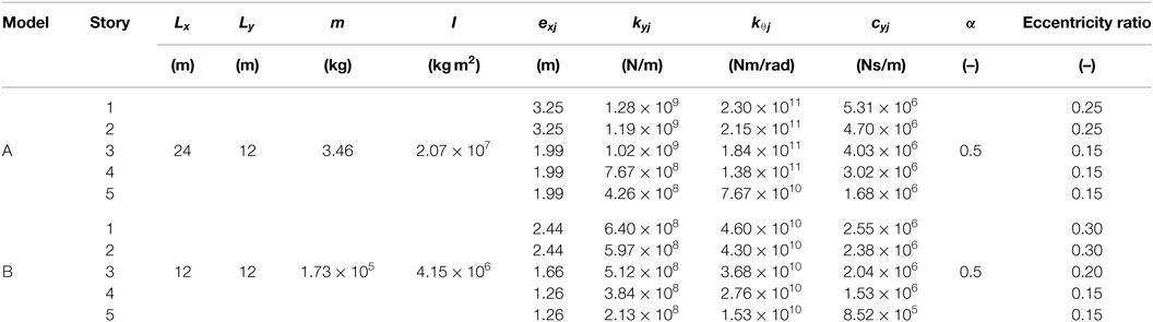
Table 1. Physical properties of torsionally coupled building.

To take into account the influence of measurement noise level on the accuracy of identification, the data generated by using the following equation were used.

$\text{Noise level}=\frac{\text{RMS value of band limited white noise}}{\text{RMS value of signal without noise}}.$ (16)

Noise-free data and data with 5% noise were used for identification. The band-limited white noise was added to the response analysis results and the input ground motions.

Prediction of Distance of Eccentricity

To predict the distance of eccentricity, it was varied parametrically and the identification functions for torsional stiffness were investigated. Figures 3A and 4A show the identification functions for torsional stiffness in the first story for the model A and model B without noise. In addition, Figures 3B and 4B indicate the identification functions for torsional stiffness in the first story for the model A and model B with noise of 5%. It can be observed that the functions exhibit horizontal constant distributions for the true distance of eccentricity (e_x = 3.254 m for model A and 2.438 m for model B).

FIGURE 3

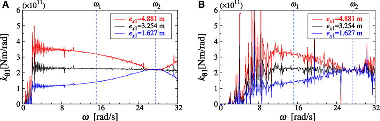
Figure 3. Identification result of torsional stiffness (model A), (A) noise level 0%, (B) noise level 5%.

FIGURE 4

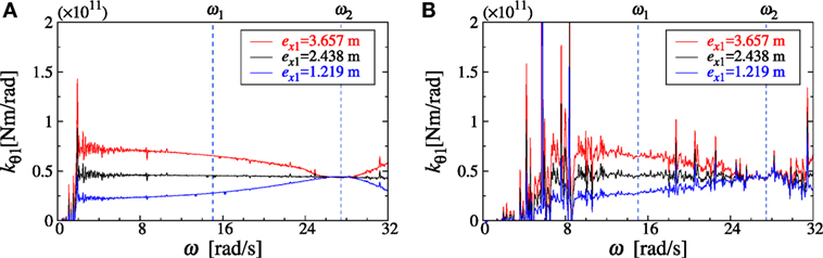
Figure 4. Identification result of torsional stiffness (model B), (A) noise level 0%, (B) noise level 5%.

Identification of Lateral Stiffness and Lateral Damping Coefficient

By using the distance of eccentricity predicted in Section “Prediction of distance of eccentricity,” the lateral stiffness is identified first. Figures 5A and 6A show the real part of the lateral identification functions defined in Eq. 12 for identification of lateral stiffness in the first story for the model A and model B without noise. Furthermore Figures 5B and 6B indicate the real part of the lateral identification functions defined in Eq. 12 for identification of lateral stiffness in the first story for the model A and model B with noise of 5%. It can be observed that the functions exhibit horizontal constant distributions around 8–20 rad/s, which indicate the lateral stiffness in the first story. When the noise is free, the function exhibits a constant value in a wide range. On the other hand, when the noise exists, it shows a stable constant value even in a narrow range.

FIGURE 5

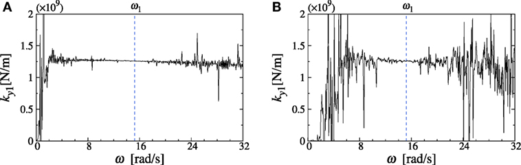
Figure 5. Identification result of lateral stiffness (model A), (A) noise level 0%, (B) noise level 5%.

FIGURE 6

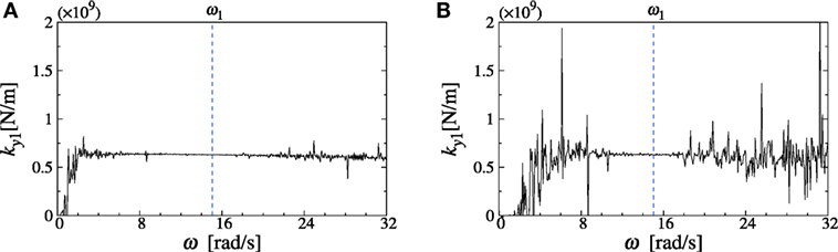
Figure 6. Identification result of lateral stiffness (model B), (A) noise level 0%, (B) noise level 5%.

Figures 7A and 8A show the imaginary part, divided by circular frequency, of the lateral identification functions defined in Eq. 12 for identification of lateral damping coefficient in the first story for the model A and model B without noise. Furthermore, Figures 7B and 8B indicate the imaginary part, divided by circular frequency, of the lateral identification functions defined in Eq. 12 for identification of lateral damping coefficient in the first story for the model A and model B with noise of 5%. It can be seen that the identification of damping is rather unstable compared to the identification of stiffness.

FIGURE 7

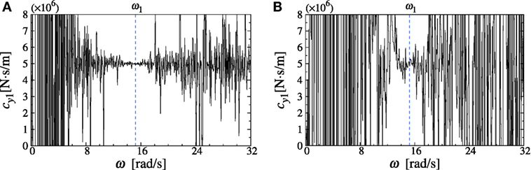
Figure 7. Identification result of lateral damping coefficient (model A), (A) noise level 0%, (B) noise level 5%.

FIGURE 8

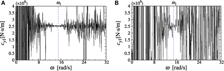
Figure 8. Identification result of lateral damping coefficient (model B), (A) noise level 0%, (B) noise level 5%.

While the previous approach using the special identification function has a difficulty in conducting the limit manipulation at zero frequency due to the influence of noise, the proposed method enables the evaluation of the identified value around the fundamental natural frequency having a smooth property. This makes the proposed method robust for noise.

Table 2 shows the identified values of lateral stiffness and lateral damping coefficient in each story for the model A and B without and with noise. The values in the parenthesis indicate the ratios of the identified values to the true values. It can be found that the errors in lateral stiffness are within 2% for all the noise levels. However, it can also be observed that the errors in lateral damping coefficient are larger than those in lateral stiffness. This phenomenon is compatible with usual identification results.

TABLE 2

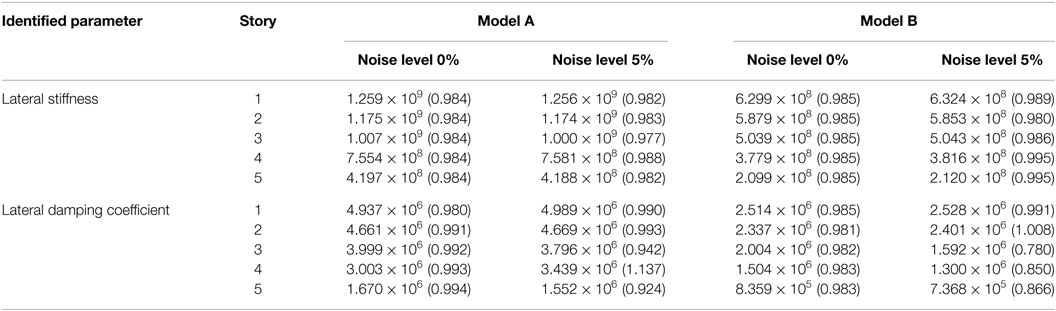
Table 2. Identified value of lateral stiffness (N/m) and lateral damping coefficient (Ns/m) in each story (number in parenthesis: ratio to the true value).

Verification of Accuracy of the Proposed Method Using Scaled Experiment

To verify the accuracy of the proposed identification method, the static test and the shaking table test have been conducted. The static test identified the lateral stiffnesses and those values are used as reference values for the identification using the shaking table tests.

Experimental Setup

Figure 9 shows the experimental set-up of a scaled two-story shear building model. Each story consists of two acrylic columns and two styrene columns. Each two columns have the same stiffness. Let k_yj, k_Sj, k_Fj denote the j-th story stiffness in the y-direction, the stiff-side story stiffness, and the flexible-side story stiffness. The y-directional accelerations at the stiff-side and the flexible-side of all the floors and that on the ground floor are measured.

FIGURE 9

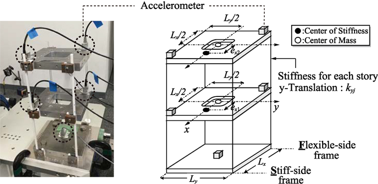
Figure 9. Experimental setup.

Identification of Lateral Stiffness by Static Test

Formulation of Lateral Stiffness

Figure 10 shows the overview of the static loading test. Let P_Fj, P_Sj denote the loads at the flexible-side and the stiff-side in the j-th story as shown in Figure 11. The springs in Figure 11 represent the stiffnesses of columns in the experimental setup shown in Figure 9. It is assumed that P_Fj and P_Sj are applied independently as shown in Figure 11. Let δ_Fj, δ_Sj denote the inter-story drift at the flexible-side subjected to P_Fj and that at the stiff-side subjected to P_Sj in the j-th story.

FIGURE 10

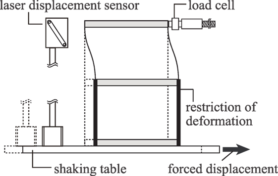
Figure 10. Static loading test.

FIGURE 11

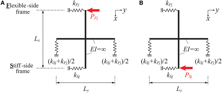
Figure 11. Mechanical model and loading condition for horizontal stiffness identification, (A) loading case of P_Fj, (B) loading case of P_Sj.

The apparent story stiffnesses of the stiff-side and the flexible-side are defined by

$\begin{array}{ll}\hfill {\overline{k}}_{\mathit{Sj}}& =\frac{P_{\mathit{Sj}}}{{\mathrm{\delta }}_{\mathit{Sj}}},\end{array}$ (17a)

$\begin{array}{ll}\hfill {\overline{k}}_{\mathit{Fj}}& =\frac{P_{\mathit{Fj}}}{{\mathrm{\delta }}_{\mathit{Fj}}}.\end{array}$ (17b)

The lateral stiffness k_yj will be expressed in terms of the above-defined apparent story stiffnesses ${\overline{k}}_{\mathit{Sj}}$, ${\overline{k}}_{\mathit{Fj}}$ of the stiff-side and the flexible-side in the following.

The inter-story drifts δ_Fj, δ_Sj at the flexible-side and the stiff-side in the j-th story can be obtained by solving the statically indeterminate structures defined in Figure 11. By substituting δ_Fj, δ_Sj into Eqs 17a,b, the apparent story stiffnesses ${\overline{k}}_{\mathit{Sj}}$, ${\overline{k}}_{\mathit{Fj}}$ of the stiff-side and the flexible-side can be related to the actual story stiffnesses k_Sj and k_Fj as follows.

$\begin{array}{l}\hfill {\overline{k}}_{\mathit{Fj}}=\frac{{\left(k_{\mathit{Sj}}+k_{\mathit{Fj}}\right)}^2+4k_{\mathit{Sj}}{k}_{\mathit{Fj}}}{5k_{\mathit{Sj}}+k_{\mathit{Fj}}},\end{array}$ (18a)

$\begin{array}{l}\hfill {\overline{k}}_{\mathit{Sj}}=\frac{{\left(k_{\mathit{Sj}}+k_{\mathit{Fj}}\right)}^2+4k_{\mathit{Sj}}{k}_{\mathit{Fj}}}{k_{\mathit{Sj}}+5k_{\mathit{Fj}}}.\end{array}$ (18b)

In Eqs 18a,b, the relation L_x/L_y = 1 is used. From Eqs 18a,b, the following relation can be derived.

${\overline{k}}_{\mathit{Fj}}\left(5k_{\mathit{Sj}}+k_{\mathit{Fj}}\right)={\overline{k}}_{\mathit{Sj}}\left(k_{\mathit{Sj}}+5k_{\mathit{Fj}}\right).$ (19)

If we introduce a coefficient r_j defined by k_Fj = r_jk_Sj, it can be expressed by

$r_j=\frac{{\overline{k}}_{\mathit{Sj}}-5{\overline{k}}_{\mathit{Fj}}}{{\overline{k}}_{\mathit{Fj}}-5{\overline{k}}_{\mathit{Sj}}}.$ (20)

Finally, k_Sj is expressed by

$k_{\mathit{Sj}}=\frac{r_j+5}{r_j^2+6r_j+1}{\overline{k}}_{\mathit{Fj}}.$ (21)

K_Fj can be derived by using k_Fj = r_jk_Sj and k_yj can then be obtained as follows.

$k_{\mathit{yj}}=k_{\mathit{Fj}}+k_{\mathit{Sj}}=\frac{\left(r_j+1\right)\left(r_j+5\right)}{r_j^2+6r_j+1}{\overline{k}}_{\mathit{Fj}}.$ (22)

Load–Deformation Relation and Prediction of Lateral Stiffness

Figures 12A,B show the force-deformation relations in the first story and the second story of the stiff-side and flexible-side frames derived by the static test. The static test was conducted cyclically (three cycles) and those data were analyzed statistically by using the least-squares method. The dotted lines indicate the least-squares fit. The symbol ρ indicates the correlation coefficient. It can be observed that the force-deformation relation of each frame is linear up to about 5 mm (1/30 rad).

FIGURE 12

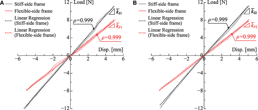
Figure 12. Load–deformation relation in each story, (A) first story, (B) second story.

The results from the least-squares fit are employed as the lateral stiffnesses ${\overline{k}}_{\mathit{Sj}},{\overline{k}}_{\mathit{Fj}}$ of frames in the stiff-side and the flexible-side in the j-th story. Those lateral stiffnesses identified from the static loading test are shown in Table 3.

TABLE 3

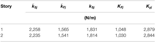
Table 3. Lateral stiffness identified from static loading test.

Identification of Lateral Stiffness by Shaking Table Experiment

The parameters of the experimental model are shown in Table 4. It was assumed that the center of mass exists at the center of the floor and the parameter α = 0.5 was used. Four ground motions (El Centro NS 1940, Taft EW 1952, Hachinohe NS 1968, Band-limited white noise) with the maximum acceleration 0.4 m/s² were employed as the input ground motions. The sampling time increment is 0.01 s.

TABLE 4

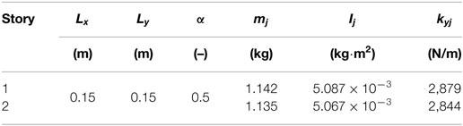
Table 4. Parameters of experimental model.

Prediction of Distance of Eccentricity

The distance of eccentricity was predicted by using the identification function for torsional stiffness. Figure 13 shows an example. The fundamental and second natural circular frequencies, ${\widehat{\mathrm{\omega }}}_1=30.2\left(\text{rad/s}\right)$ and ${\widehat{\mathrm{\omega }}}_2=43.5\left(\text{rad/s}\right)$, are also plotted in Figure 13. It can be observed that the distance of eccentricity is 0.0102 m in the first story and 0.0103 m in the second story. Using these distances of eccentricity, the lateral stiffnesses are identified next.

FIGURE 13

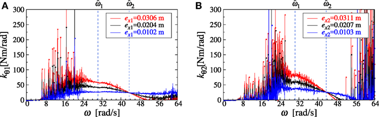
Figure 13. Identification results of torsional stiffness, (A) first story, (B) second story.

Identification of Lateral Stiffness

The identification results of the lateral stiffness (Eq. 12) are shown in Figures 14A,B, and the identified lateral stiffnesses are shown in Table 5. The values in the parenthesis indicate the ratios of the identified values to the true values. It can be observed that, as in the numerical investigations, the identification results are stable around the fundamental natural frequency, i.e., exhibits a horizontally constant property. In addition, the maximum discrepancy is within 5%, and it may be concluded that the proposed method is rather accurate and reliable. As for damping, the property of damping (stiffness-proportional or not) may be uncertain in the actual situation. The identification of damping in actual situation will be investigated in future.

FIGURE 14

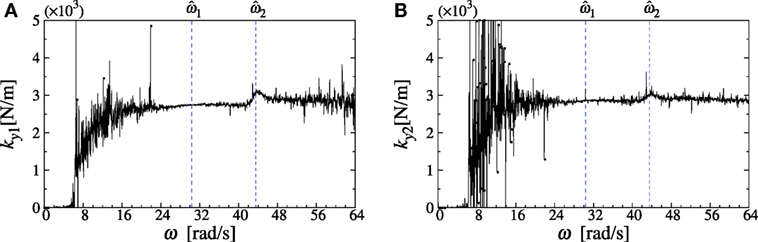
Figure 14. Identification results of lateral stiffness, (A) first story, (B) second story.

TABLE 5

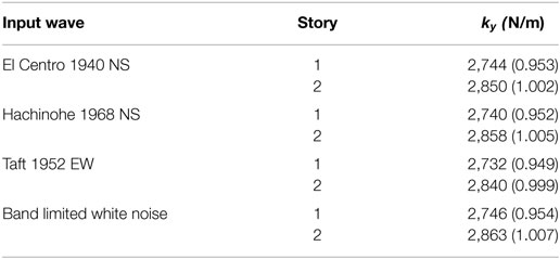
Table 5. Identified value of horizontal stiffness in each story under various input waves.

Conclusion

A new method of frequency-domain physical-parameter SI has been developed for three-dimensional building structures with stiffness eccentricity. The conclusions may be summarized as follows.

(1) The dynamic equilibrium of the free body above the j-th story can be used to identify the j-th story stiffness and damping. It is required to measure the horizontal and rotational accelerations at all stories to identify the story stiffnesses and damping coefficients of all stories. Compared to the previous approach using the special identification function, the limit manipulation at zero frequency is unnecessary and this makes the proposed method robust for noise. It should be reminded that, even if we try to derive the special identification function for 3D building structures including the limit manipulation, it seems difficult to obtain such identification function because of the complexity of governing equations for models with eccentricity.

(2) The quantities of eccentricities of all stories can be identified using the slopes of the functions (called the identification functions) for identification of torsional stiffness in frequency domain. If the true distance of eccentricity is given, the real part and the imaginary part, divided by circular frequency, of the lateral identification functions become constant with respect to frequency. On the contrary, if an erroneous distance of eccentricity is used, those functions are not constant. This property can be used for the identification of the distance of eccentricity.

(3) Numerical investigation demonstrated that the proposed identification method is reliable and possesses an acceptable accuracy. However, it should be noted that the identification of damping is rather unstable compared to the identification of stiffness as usual in general identification problems.

(4) Experiments using scaled models made clear the reliability and accuracy of the proposed identification method.

Author Contributions

KN formulated the problem, conducted the computation and experiment, and wrote the paper. IT supervised the research and wrote the paper.

Funding

Part of the present work is supported by the JSPS KAKENHI (No. 15H04079, 17J00407). This support is greatly appreciated.

Conflict of Interest Statement

The authors declare that the research was conducted in the absence of any commercial or financial relationships that could be construed as a potential conflict of interest.

References

Agbabian, M. S., Masri, S. F., Miller, R. K., and Caughey, T. K. (1991). System identification approach to detection of structural changes. J. Eng. Mech. 117, 370–390. doi: 10.1061/(ASCE)0733-9399(1991)117:2(370)

CrossRef Full Text | Google Scholar

Boller, C., Chang, F.-K., and Fujino, Y. (eds) (2009). Encyclopedia of Structural Control and Health Monitoring, Vol. 1-5. Chichester: Wiley.

Google Scholar

Brownjohn, J. M. W. (2003). Ambient vibration studies for system identification of tall building. Earth Eng. Struct. Dyn. 32, 71–95. doi:10.1002/eqe.215

CrossRef Full Text | Google Scholar

Fujita, K., Fujimori, Y., and Takewaki, I. (2017). Modal-physical hybrid system identification of high-rise building via subspace method and inverse-mode method. Front. Built Environ. 3:51. doi:10.3389/fbuil.2017.00051

CrossRef Full Text | Google Scholar

Fujita, K., Ikeda, A., Shirono, M., and Takewaki, I. (2013). “System identification of high-rise buildings using shear-bending model and ARX model: experimental investigation,” in Proc. of ICEAS13 in ASEM13 (Jeju, Korea), 2803–2815. September 8-12.

Google Scholar

Fujita, K., Ikeda, A., and Takewaki, I. (2015). Application of story-wise shear building identification method to actual ambient vibration. Front. Built Environ. 1:2. doi:10.3389/fbuil.2015.00002

CrossRef Full Text | Google Scholar

Hart, G. C., and Yao, J. T. P. (1977). System identification in structural dynamics. J. Eng. Mech. Div 103, 1089–1104.

Google Scholar

Hjelmstad, K. D. (1996). On the uniqueness of modal parameter estimation. J. Sound Vib. 192, 581–598. doi:10.1006/jsvi.1996.0205

CrossRef Full Text | Google Scholar

Hjelmstad, K. D., Banan, M. O. R., and Banan, M. A. R. (1995). On building finite element models of structures from modal response. Earthquake Eng. Struct. Dyn. 24, 53–67.

Google Scholar

Hoshiya, M., and Saito, E. (1984). Structural identification by extended Kalman filter. J. Eng. Mech. 110, 1757–1770. doi:10.1061/(ASCE)0733-9399(1984)110:12(1757)

CrossRef Full Text | Google Scholar

Ikeda, A., Fujita, K., and Takewaki, I. (2014). Story-wise system identification of actual shear building using ambient vibration data and ARX model. Earthquakes Struct. 7, 1093–1118. doi:10.12989/eas.2014.7.6.1093

CrossRef Full Text | Google Scholar

Ikeda, A., Fujita, K., and Takewaki, I. (2015). Reliability of system identification technique in super high-rise building. Front. Built Environ. 1:11. doi:10.3389/fbuil.2015.00011

CrossRef Full Text | Google Scholar

Johnson, E., and Wojtkiewicz, S. (2014). Efficient sensitivity analysis of structures with local modifications. II: transfer functions and spectral densities. J. Eng. Mech. 140. doi:10.1061/(ASCE)EM.1943-7889.0000769

CrossRef Full Text | Google Scholar

Kuwabara, M., Yoshitomi, S., and Takewaki, I. (2013). A new approach to system identification and damage detection of high-rise buildings. Struct. Control Health Monitor. 20, 703–727. doi:10.1002/stc.1486

CrossRef Full Text | Google Scholar

Maeda, T., Yoshitomi, S., and Takewaki, I. (2011). Stiffness-damping identification of buildings using limited earthquake records and ARX model. J. Struct. Const. Eng. 666, 1415–1423. (in Japanese). doi:10.3130/aijs.76.1415

CrossRef Full Text | Google Scholar

Minami, Y., Yoshitomi, S., and Takewaki, I. (2013). System identification of super high-rise buildings using limited vibration data during the 2011 Tohoku (Japan) earthquake. Struct. Control Health Monitor. 20, 1317–1338. doi:10.1002/stc.1537

CrossRef Full Text | Google Scholar

Nagarajaiah, S., and Basu, B. (2009). Output only modal identification and structural damage detection using time frequency & wavelet techniques. Earthquake Eng. Eng. Vib. 8, 583–605. doi:10.1007/s11803-009-9120-6

CrossRef Full Text | Google Scholar

Nakamura, M., and Yasui, Y. (1999). Damage evaluation of a steel structure subjected to strong earthquake motion based on ambient vibration measurements. J. Struct. Construct. Eng. 517, 61–68. (in Japanese). doi:10.3130/aijs.64.61_1

CrossRef Full Text | Google Scholar

Omrani, R., Hudson, R. E., and Taciroglu, E. (2012). Story-by-story estimation of the stiffness parameters of laterally-torsionally coupled buildings using forced or ambient vibration data: I. Formulation and verification. Earth Eng. Struct. Dyn. 41, 1609–1634. doi:10.1002/eqe.1192

CrossRef Full Text | Google Scholar

Shinozuka, M., and Ghanem, R. (1995). Structural-system identification II: experimental verification. J. Eng. Mech. 121, 265–273. doi:10.1061/(ASCE)0733-9399(1995)121:2(265)

CrossRef Full Text | Google Scholar

Shintani, K., Yoshitomi, S., and Takewaki, I. (2017). Direct linear system identification method for multi-story three-dimensional building structure with general eccentricity. Front. Built Environ. 3:17. doi:10.3389/fbuil.2017.00017

CrossRef Full Text | Google Scholar

Takewaki, I., and Nakamura, M. (2000). Stiffness-damping simultaneous identification using limited earthquake records. Earth. Eng. Struct. Dyn. 29, 1219–1238. doi:10.1002/1096-9845(200008)29:8<1219::AID-EQE968>3.0.CO;2-X

CrossRef Full Text | Google Scholar

Takewaki, I., and Nakamura, M. (2005). Stiffness-damping simultaneous identification under limited observation. J. Eng. Mech. 131, 1027–1035. doi:10.1061/(ASCE)0733-9399(2005)131:10(1027)

CrossRef Full Text | Google Scholar

Takewaki, I., and Nakamura, M. (2010). Temporal variation of modal properties of a base-isolated building during an earthquake. J. Zhejiang Univ. Sci. A 11, 1–8. doi:10.1631/jzus.A0900462

CrossRef Full Text | Google Scholar

Takewaki, I., Nakamura, M., and Yoshitomi, S. (2011). System Identification for Structural Health Monitoring. UK: WIT Press.

Google Scholar

Udwadia, F. E., Sharma, D. K., and Shah, P. C. (1978). Uniqueness of damping and stiffness distributions in the identification of soil and structural systems. J. Appl. Mech. 45, 181–187. doi:10.1115/1.3424224

CrossRef Full Text | Google Scholar

Wojtkiewicz, S., and Johnson, E. (2014). Efficient sensitivity analysis of structures with local modifications. I: time domain responses. J. Eng. Mech. 140. doi:10.1061/(ASCE)EM.1943-7889.0000768

CrossRef Full Text | Google Scholar

Zhang, D., and Johnson, E. (2013). Substructure identification for shear structures I: substructure identification method. Struct. Control Health Monitor. 20, 804–820. doi:10.1002/stc.1497

CrossRef Full Text | Google Scholar