Response Analysis and Auto-Regressive Exogenous Modeling of a Steel-Reinforced Concrete High-Rise Building during the 2011 Off the Pacific Coast of Tohoku Earthquake

Introduction

The 2011 off The Pacific Coast of Tohoku Earthquake on March 11 caused considerable damage to a wide area of eastern Japan [USGS, 2016; Architectural Institute of Japan (AIJ), 2011; Kawase, 2014]. A large number of related earthquake observation records were obtained at various places. Of importance for seismic design are the records from buildings, since there are typically very few records of this type obtained in Japan. To design more earthquake-resistant buildings and improve disaster prevention, it is necessary to use these data for analysis and evaluation of the behavior of buildings subjected to destructive, earthquake-induced vibrations.

There have been many studies in this regard, such as Okawa et al. (2013), who showed practical design implications of various types of earthquake-response records collected from buildings during the Tohoku earthquake. Nakamura et al. (2016) studied the horizontal first-mode vibration characteristics of low- and middle-rise reinforced concrete (RC) and steel-reinforced concrete (SRC) buildings. These authors showed that amplitude dependency was evident in both the natural mode and the damping ratio. Uebayashi et al. (2016) observed many ambient seismic records in RC high-rise buildings before and after strong ground motion, including the Tohoku earthquake, and proposed a simple damage equation to evaluate the stiffness degrading ratio. Çelebi et al. (2016) studied the behavior of a 37-story building in Tokyo during the Tohoku earthquake based on seismic records and showed that the building was not structurally damaged.

This paper presents an earthquake-response simulation analysis (hereinafter referred to as a seismic response analysis) conducted using data recorded during the main shock of the Tohoku earthquake, and other seismic data recorded before and after the earthquake. The data were obtained in a high-rise SRC building in the Tokyo Bay area, from which the vibration characteristics of the building were identified. The shaking behavior and vibration characteristics of the building were then estimated from the data and analysis.

An overview of the building is first presented, along with the characteristics of earthquake motion and building motion during the main shock, which indicate a change in the natural period before and after the earthquake. Next, the results of the seismic response analysis are presented, including the analytical model and conditions, as well as a comparison of the observed records with the analytical results.

Using the analytical results, the effects of the soil structure on the response of the building to ground motion is examined. An auto-regressive exogenous (ARX) model (Safac, 1992; Loh and Lin, 1996; Saito, 1998; Ikeda et al., 2014; Ikeda, 2016) is then used to identify the characteristics of the building during the earthquake, such as the first and the second natural periods and damping ratios. The analytical results are then compared with the observational records to evaluate the accuracy of the response analysis.

Overview of the Building and Soil

The building studied is a 32-story SRC frame structure high-rise (Figure 1A) situated in Tokyo Bay (Nakamura et al., 2013). This area is known to be underlain by thick and soft Holocene sedimentary layers (Table 1).

FIGURE 1

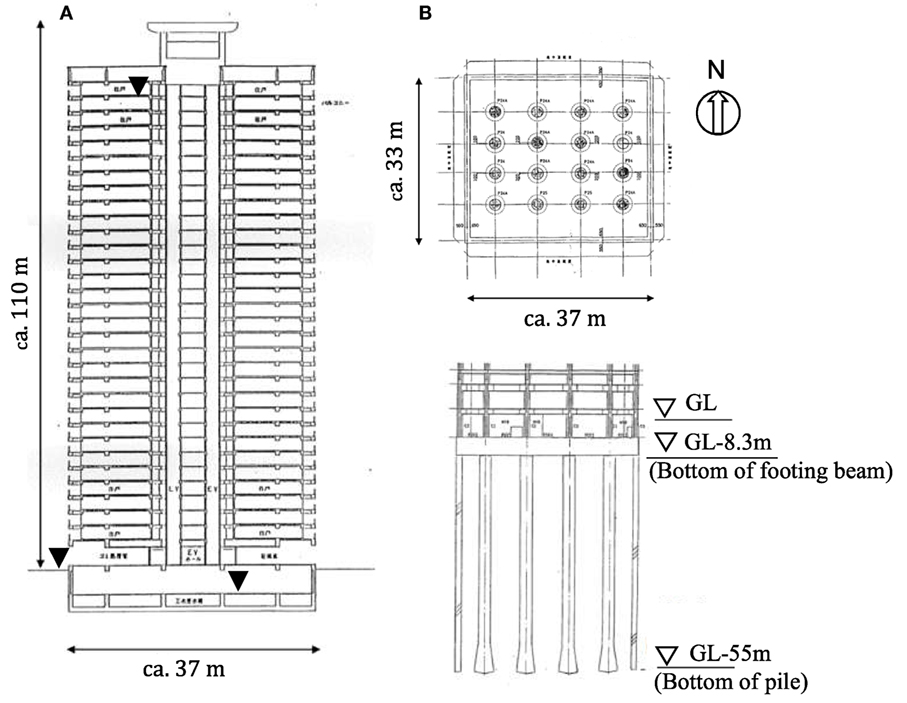
Figure 1. Profile of 32-story steel-reinforced concrete building. (A) Section of the frame structure high-rise (▼: Observation points). (B) Plan view and section view of substructure.

TABLE 1

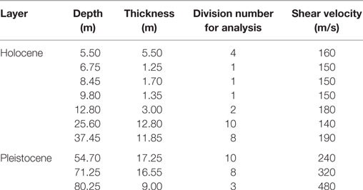
Table 1. Parameters of soil underlying the Tokyo Bay area.

The substructure of the building consists of diaphragm walls that are 1.2 m thick, which provide a large horizontal resistive force during earthquakes. These are installed cylindrically around the building, with 16 belled piles installed underneath the building to provide vertical support. These piles are supported by the diluvial Edogawa Formation sand layer that occurs 55 m below ground level (GL) (Figure 1B).

Earthquake Observation Results and Building Characteristics

Seismic readings were taken at GL, the first basement floor level (B1F), and the 32nd floor level (32F) of the building. Table 2 shows the natural period of the building in an N–S direction, which was calculated using the largest acceleration response at each of the three positions and a transfer function for 32F/B1F.

TABLE 2

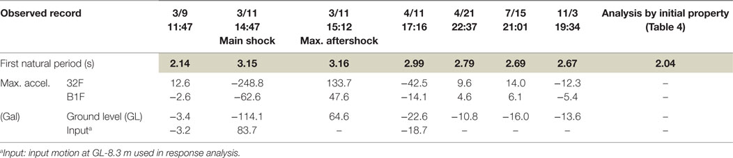
Table 2. Temporal changes in the transfer function according to the natural periods of the building (N–S direction).

The natural period during the earthquake on March 9 (referred to as the 3/9 pre-shock) was 2.14 s, which is close to the analyzed natural period using the initial property (2.04 s), which is explained in Section “Model Overview.” The natural period was 3.16 s during both the main shock and the largest aftershock on March 11 (the 3/11 aftershock). However, the earthquake on November 3 had a period of 2.67 s. The natural period of the building showed almost the same pattern in the E–W direction.

The main shock registered an upper 5 on the Japanese seismic intensity scale in the Tokyo Bay area. The maximum acceleration recorded at GL was 114 Gal in the N–S direction and 127 Gal in the E–W direction. This observed wave was withdrawn to the level of the diluvial surface (55 m below GL) by using one-dimensional wave propagation theory (SHAKE) by Schnabel et al. (1972) to allow for comparison with the response spectrum of the Japanese design basis waves (Figure 2). The observed wave was between a Level 1 and Level 2 earthquake. According to the Japanese building code, buildings must remain in an elastic condition for Level 1 earthquakes, and during Level 2 earthquakes they must not collapse.

FIGURE 2

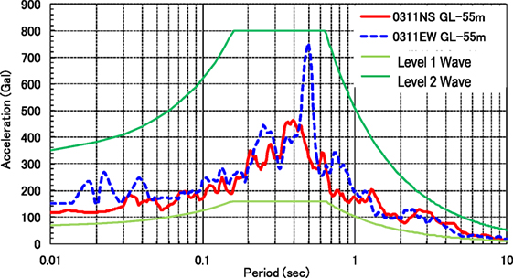
Figure 2. Comparison of acceleration spectra between the 3/11 main shock and the Japanese design earthquakes of Level 1 and Level 2.

The building transformed by about 40 cm between B1F and 32F in both N–S and E–W directions during the main shock, as calculated from the integrated values of acceleration. This corresponds to about 1/250 of the average drift angle of the building. Although this earthquake caused some cracks to appear in the beams of each floor, the overall damage was minor.

Analytical Seismic Response Model

Model Overview

The analytical model used in this study is a sway-rocking (SR) model, as shown in Figure 3A. The superstructure used in the analysis is a non-linear multistory lumped-mass shear beam model, constructed according to the N–S and E–W directions of the 32-story building. Two types of springs were used as the ground SR spring: the first has initial properties based on the ground survey records relevant to the building and the second accounts for non-linearity during the main shock. Waves observed at GL are extrapolated to the bottom of a footing beam in the model (8.3 m below GL) using SHAKE.

FIGURE 3

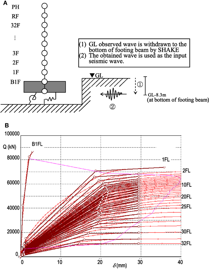
Figure 3. Structure model. (A) Analytical sway-rocking model, with the seismic motion input method described. (B) Skeleton curves (N–S direction) showing the first breaking point for each story, which correspond to the cracking points, and the second breaking points which correspond to the yield points.

In this study, response analysis was conducted on the observed motions of the 3/9 pre-shock, the 3/11 main shock, and the April 11 earthquake aftershocks (the 4/11 earthquake). Table 2 presents a summary of the relevant earthquake and aftershock data. The duration of the analysis was 300 s, including the main shaking parts of the earthquakes with 0.01 s time steps. The Newmark-β method (β = 0.25) was used for time integration.

The spring that takes non-linearity into account was used as the ground SR spring for the main shock, while the spring with the initial properties was used for the other earthquakes.

Superstructure Model

To calculate the skeleton curve of the superstructure a 3D frame model was created to replace the columns and crossbeams of the building with beam elements, allowing for incremental static load (pushover) analysis to be performed. The 3D frame model was used only for static analysis, and the external force distribution was set based on the results of auxiliary response analysis conducted at the time of model design. An element with a rigid-plastic rotational spring and rigid zones at both ends was used for the columns and crossbeams. The elastic stiffness was derived from the concrete, with Young’s modulus calculated from the design strength, and the built-in steel beam. A tri-linear bending property was used and was assumed to contain cracks. Finally, an asymmetric bi-linear column axial property was used.

Based on the result of the pushover analysis, the drift angle–shearing force relationship for each story was fitted to the tri-linear properties. Figure 3B shows the result of the calculation in the N–S direction, in which it is evident that the first breaking point in the skeleton curves of each story corresponds to the cracking point, while the second breaking point corresponds to the yield point.

Ground Response Analysis

Waves from the earthquakes observed at GL were extrapolated to the bottom of a footing beam (8.3 m below GL) by using SHAKE. The ground model was set up according to the lithological data presented in Table 1, with 1.5 m intervals to a depth of 80.25 m below GL. The HD non-linear ground model (Hardin and Drnevich, 1972) was used, based on the following calculations:

$G/G_0=\frac{1}{1+\gamma /{\gamma }_{0.5}}$ (1)

$h=h_{\text{max}}(1-G/G_0)$ (2)

where the lower limit of the damping ratio was set to 2%, γ_0.5 = 0.18% (for clay soil), h_max = 17% (for clay soil), γ_0.5 = 0.10% (for sandy soil), h_max = 21% (for sandy soil), G = shear modulus, G₀ = initial shear modulus, γ = shear strain, and γ_0.5 = reference strain.

The response wave at the bottom of the footing beam at 8.3 m below GL was obtained from the sum of the upward wave (E) and downward wave (F) calculated in SHAKE and input into the analysis. The bottom line of Table 2 shows the maximum acceleration calculated for the input wave. In all earthquakes analyzed in this study, the maximum acceleration of the input wave was slightly lower than that at GL.

Figure 4A shows the shear strain values obtained from the analysis of the main shock, Figure 4B shows the shear wave velocity calculated from the shear strain, and Figure 4C shows the damping ratio. Figures 4B,C also show the initial properties of the spring system before the shock occurred. Figure 4A shows that the maximum shear strain in the ground was 0.1%, and that liquefaction was unlikely to occur.

FIGURE 4

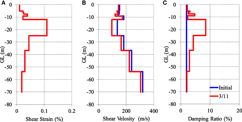
Figure 4. Results of the soil response analysis of the 3/11 main shock (average of N–S and E–W directions) showing (A) maximum shear strain, (B) shear wave velocity calculated from shear strain, and (C) damping ratio.

The analysis was conducted in both N–S and E–W directions, with relatively little difference between the two. Figure 4 also shows the average values of the response properties of each story in both directions.

A soil spring was then established using the response result. The axisymmetric finite element model analytical program, Super FLUSH (Family Soil-Structure Interaction Analysis, Jishin Kougaku Kenkyusho Inc., 2003) was used to calculate the frequency domain. Figure 5A shows an image of the axisymmetric model, and the following is an outline of the analytical conditions:

(1) An axisymmetric model of the central axis of a building was considered.

(2) For the basement floors (GL to 8.3 m below GL), a massless rigid body was adopted, and defined as an equivalent cylinder.

(3) For the ground properties, both initial properties and the equivalent linear values of the 3/11 main shock were used.

(4) A diaphragm wall was defined as a cylindrical element with equivalent radius and plate thickness of 1.2 m. A pile group was defined by multiplex ring pile elements (equivalent to the cylindrical element) with a plate thickness of 1.2 m. Both elements were modeled to 55 m below GL.

(5) The ground below the building was divided vertically into segments 1.5 m tall, to a depth of 80.25 m below GL (similar to the SHAKE model). The ground was radially segmented into 1 m segments from the center to 80 m below GL. The sides and base of the model were considered to be viscous boundaries.

(6) The ground impedances of sway and rocking were considered to be uncoupled from one another and were obtained by acquiring the reciprocal of compliance. This was determined from the forced excitation of the rigid, massless body.

(7) The frequency range analyzed was 0.1–10 Hz, in increments of 0.1 Hz.

FIGURE 5

Figure 5. Modeling of underground part. (A) Schematic diagram of the model used for axisymmetric analysis, (B) calculated sway impedance, and (C) rocking impedance.

Figures 5B,C show the sway and rocking impedance values obtained from the analysis. The value of the soil spring used for the response analysis is independent of frequency and corresponds to the impedance at 0.5 Hz, which is close in value to the first frequency of the building. Table 3 shows the values obtained from the soil spring.

TABLE 3

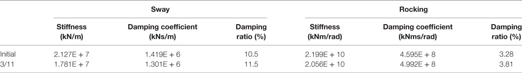
Table 3. Soil properties used for response analysis.

Eigenvalue Analysis

Table 4 shows the results of eigenvalue analysis using the SR model in the N–S direction. For comparison, the table also shows the results of a model for which the soil spring was not considered and the foundation was fixed. Figure 6 shows the participation function (in the N–S direction) of a model using an initial property SR spring. The participation function using the soil spring for the 3/11 earthquake shows similar results.

TABLE 4

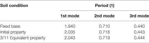
Table 4. Results of eigenvalue analysis (N–S direction).

FIGURE 6

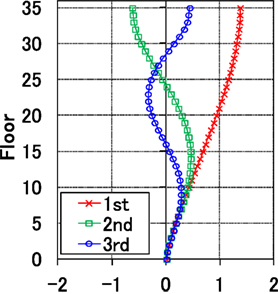
Figure 6. Participation function (N–S direction) of the model using an initial property sway-rocking spring.

The natural period of the SR model was slightly longer than that of the fixed foundation model because of the soil spring. Although the natural period of the soil spring for the 3/11 earthquake was longer than that of the initial property SR spring model, the difference was very small, showing that the effect of non-linearity of the ground was slight. The natural period in the E–W direction also shows the same pattern.

Seismic Response Analysis

The SR model was used to conduct seismic response analysis. The Takeda model was used as a hysteretic rule for each story of the building. The material damping was of the tangent stiffness-proportional type, with a damping ratio of 2%. A value of 3% is generally used for structural design of RC and SRC buildings in Japan.

Three cases were analyzed: (1) the 3/9 pre-shock, (2) the 3/11 main shock, and (3) the 4/11 aftershock. The response waves in the N–S and E–W directions at 8.3 m below GL, as calculated in Section “Ground Response Analysis,” were inputs into the model. The results of the seismic response analysis for each case are presented in the next three subsections.

The 3/9 Pre-Shock

Values of maximum acceleration and maximum displacement at 32F are shown in Table 5. The maximum displacement was obtained by double integration of the observed acceleration waveform, and parts of the earthquake period longer than 20 s were filtered out. In the N–S direction, the observed values of maximum acceleration and maximum displacement at each story correspond well with the analyzed values, as shown in Figures 7A–D. However, slight differences are evident in the E–W direction.

TABLE 5

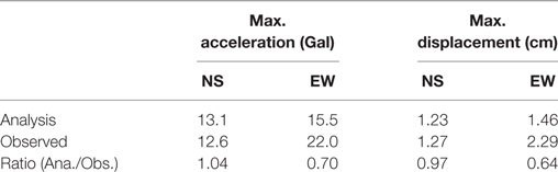
Table 5. Maximum acceleration and displacement responses at 32F (3/9 pre-shock).

FIGURE 7

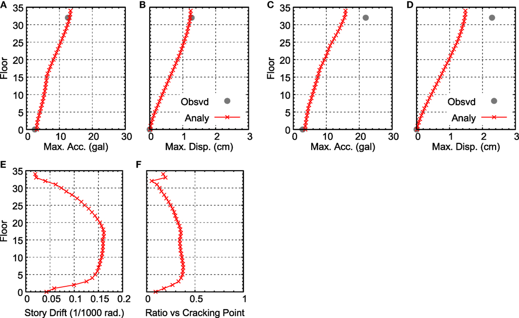
Figure 7. Comparison of maximum response for the 3/9 pre-shock: (A) maximum acceleration (N–S direction), (B) maximum displacement (N–S direction), (C) maximum acceleration (E–W direction), (D) maximum displacement (E–W direction), (E) distribution of story drift angle (N–S direction), and (F) distribution of response ratio vs. cracking point (N–S direction).

Figure 7E shows the distribution of the story drift angle of each story in the N–S direction. The story drift angle is large for stories 5–20 stories, but the angle decreases at higher stories. The maximum drift angle never exceeds 0.0002 rad. Figure 7F shows the distribution of the response ratio (the ratio of the maximum response) against the first breaking point (the cracking point) of the skeleton curve shown in Figure 3B. The response ratio is <1 for the N–S direction, indicating that the response is in the elastic region. The response ratio in the E–W direction shows a similar pattern.

The observed and analytical results of the acceleration waveform as a function of time at 32F in the N–S direction are compared in Figure 8A. The analyzed response wave corresponds well with the observed response wave in the 0- to 100-s time interval, but a slight difference is evident after 150 s. Figure 8B shows the transfer function in the N–S direction at 32F to the observed wave at GL. Parzen’s window function was used in this calculation at a bandwidth of 0.05 Hz, and although the peak position of the result differs slightly from the observed value, both results are essentially consistent.

FIGURE 8

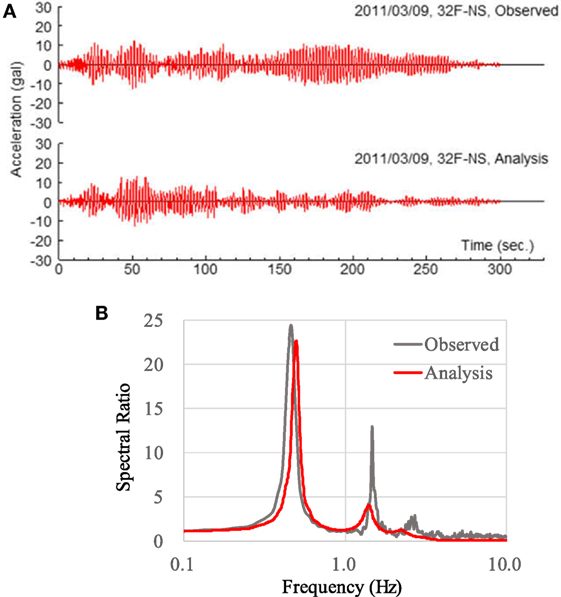
Figure 8. Comparison of observed and analytical response for the 3/9 pre-shock (N–S direction): (A) acceleration waveforms for 32F, (B) transfer function between 32F and ground level.

The 3/11 Main Shock

Maximum acceleration and maximum displacement at 32F are shown in Table 6, and the distribution of both at each story is shown in Figures 9A–D. The response results of acceleration correspond well with the observed values in the N–S direction but are lower than the response results in the E–W direction. The response results of displacement correspond well with the observed values in both directions.

TABLE 6

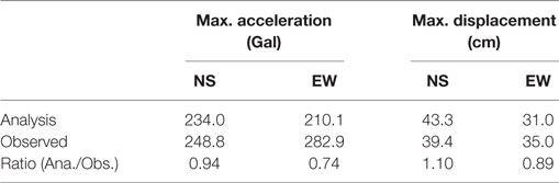
Table 6. Maximum acceleration and displacement responses at 32F (3/11 main shock).

FIGURE 9

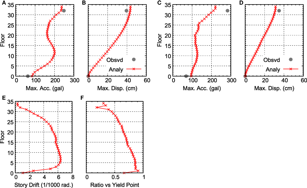
Figure 9. Comparison of maximum response for the 3/11 main shock: (A) maximum acceleration (N–S direction), (B) maximum displacement (N–S direction), (C) maximum acceleration (E–W direction), (D) maximum displacement (E–W direction), (E) distribution of story drift angle (N–S direction), and (F) distribution of ductility factor (N–S direction).

Figure 9E shows the distribution of the story drift angle in the N–S direction. The story drift angle is about 0.0065 rad, with the largest drift angle recorded in stories 5–10. Figure 9F shows the ductility factor in the N–S direction (i.e., the response ratio to the second breaking point of the skeleton curve shown in Figure 3B). The maximum response values are above the first breaking point (the cracking point) and below the second breaking point (the yield point) for all stories. This indicates that the damage to the building was comparatively minor. The base shear coefficient in the N–S direction, calculated from the maximum shearing force obtained from analytical results, is 0.118.

The observed and analytical results of the acceleration waveforms, as a function of time at 32F in the N–S direction, are presented in Figure 10A. The analyzed response wave corresponds well with the observed wave. Figure 10B shows the transfer function between 32F and GL for the N–S direction. The peak position of the observed transfer function is >0.1 Hz lower than that of the 3/9 pre-shock, and the transfer function of the analyzed response wave corresponds well with that of the observed wave.

FIGURE 10

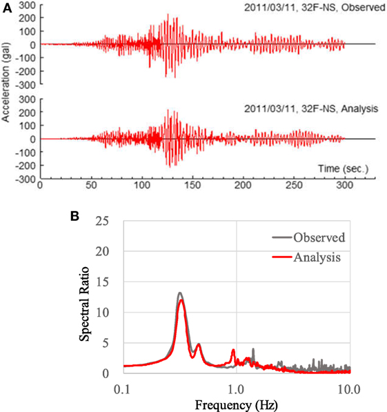
Figure 10. Comparison of observed and analytical response for the 3/11 main shock (N–S direction): (A) acceleration waveforms for 32F and (B) transfer function between 32F and ground level.

The 4/11 Earthquake

Table 7 shows the maximum acceleration and maximum displacement values at 32F, and Figures 11A–D show the distribution of each at each story. In both the N–S and E–W directions, the maximum acceleration from analytical results (referred to as “Analy1”) corresponds well with that of the observed value, and the maximum displacement value of Analy1 is noticeably lower than that of the observed value. The transfer function between 32F and GL in the N–S direction is shown in Figure 11E. The observed transfer function seems to have been affected non-linearly by the 3/11 main shock, while the value of Analy1 does not correspond with the observed value.

TABLE 7

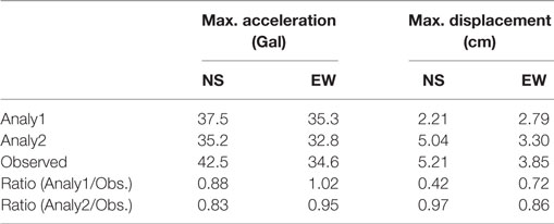
Table 7. Maximum acceleration and displacement responses at 32F (4/11 aftershock).

FIGURE 11

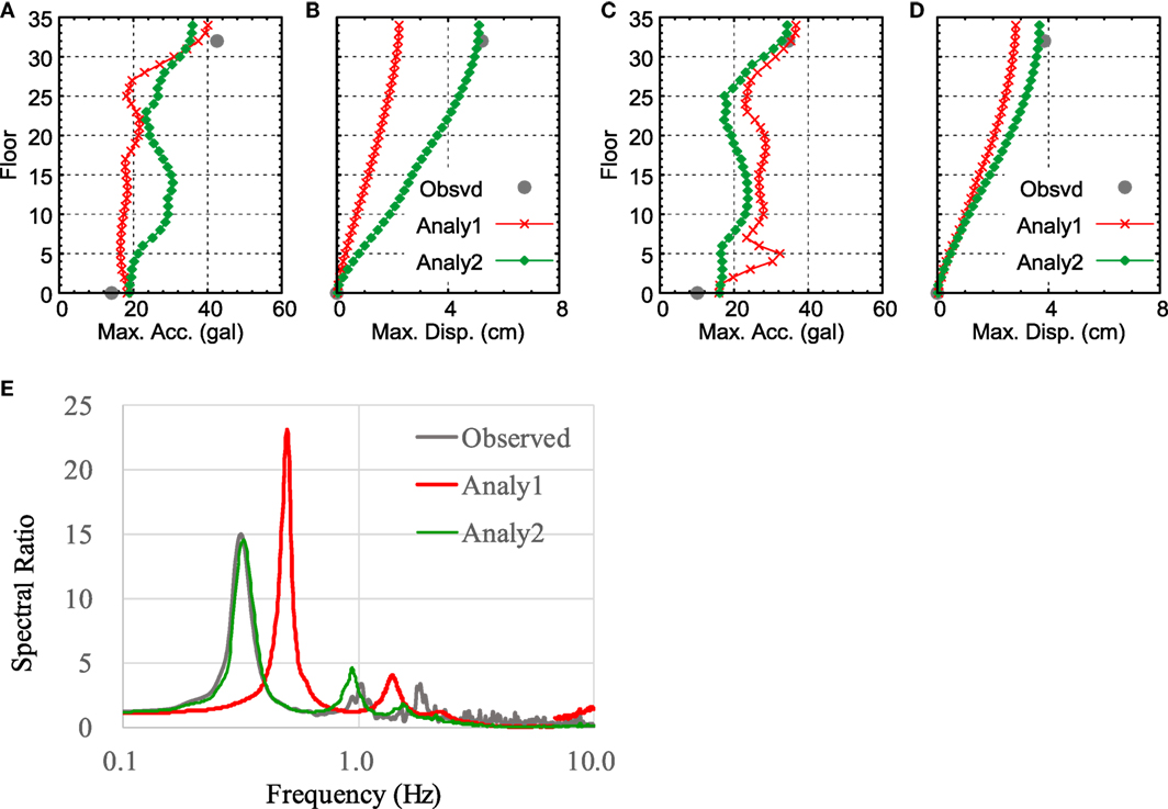
Figure 11. Comparison of maximum response for the 4/11 aftershock: (A) maximum acceleration (N–S direction), (B) maximum displacement (N–S direction), (C) maximum acceleration (E–W direction), (D) maximum displacement (E–W direction), and (E) transfer function between 32F and ground level for observed and analytical results (N–S direction).

As a result, the input waves of the 3/11 main shock and the 4/11 earthquake were connected to conduct seismic response analysis (“Analy2”). To attenuate the vibration of the first wave, 100 s of zero acceleration was inserted between both input waves of 300 s, resulting in a total wave duration of 700 s. The results of Analy2 (both 3/11 and 4/11 wave inputs) show that the maximum displacement exceeds that of Analy1 (only the 4/11 wave input) and approaches the observed value.

Figure 11E also shows the transfer function of Analy2. An initial property soil spring was used in both Analy1 and Analy2. The transfer function of the analyzed response wave was prepared using only the response values in the second half of the 700-s time period of the analysis. The peak position of the transfer function with continuous input decreased compared with that of the single input and approached the observed value.

The above shows that the effect of the non-linearity of the building caused by the 3/11 main shock needs to be considered in terms of the response of the 4/11 earthquake as well.

Effect of the Soil Spring

The effect of a soil spring on the response in the N–S direction during the 3/9 pre-shock is shown in Figure 12A. When a soil spring is included in the analysis, the resulting value corresponds well with the observed value. However, when a soil spring is not considered and the foundation is assumed to be fixed, there is a large difference in values.

FIGURE 12

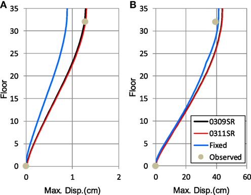
Figure 12. Comparison of soil spring effects for (A) the 3/9 pre-shock and (B) the 3/11 main shock (N–S direction).

For the 3/11 main shock, there is essentially no difference between cases with an initial property soil spring and a non-linear soil spring. This is most likely because the difference between the two spring values was also small when the non-linear level of the ground was comparatively weak during the 3/11 main shock. If the sway spring is fixed, it resulted in a limited effect on the response, showing that the rocking spring has a more significant effect on the response of a building to ground motion.

Similarly, Figure 12B shows the effect of a soil spring, in an N–S direction, on the building response during the 3/11 main shock. There is a difference of only 1 cm at the top of the building between a soil spring case and a fixed foundation case. Since the displacement at the top of the building can be as large as 40 cm because of non-linearity, the effect of the soil spring is relatively limited.

Change in the Natural Period and Damping Ratio During Vibration

Changes in the first and second natural periods and damping ratios during vibration were calculated to study the relationship between the results of response analysis and observed values. An ARX model was used for the evaluation, in which the acceleration time history waves at GL and 32F were used as input and output, respectively. Transfer functions in the calculation were obtained by dividing the time history wave at 32F by that at GL in the frequency domain. This was done for the records of both the 3/9 pre-shock and 3/11 main shock. A trapezoidal filter, which includes the shape of the first mode, was set with an upper value of 1.0. The filter was applied to the waves for both 32F and GL, followed by use of the ARX model to estimate the vibration characteristics of the first mode. The characteristics of the second mode were estimated in the same way.

Transfer functions of the 3/9 pre-shock and 3/11 main shock, and the trapezoidal filters for both the first and the second modes, are shown in Figure 13A. The same filters were used for both earthquakes. The model dimension was set to 2 because the model was transferred to the one-degree-of-freedom model by the filter, and the results of the calculation with values in the past 10 s were output every 5 s.

FIGURE 13

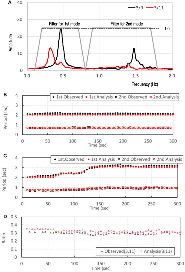
Figure 13. Auto-regressive exogenous analysis results for natural period in the N–S direction: (A) transfer functions of the 3/9 pre-shock and 3/11 main shock, and the trapezoidal filter used for both first and second modes, (B) change in first and second natural periods during the 3/9 pre-shock compared for observed and analytical results, (C) those during the 3/11 main shock, and (D) values of the second natural period divided by first natural period for both observed and analytical results during the 3/11 main shock.

The comparison between analytical results and observed values for the first and second natural periods during the 3/9 pre-shock is shown in Figure 13B. Since the response of the building was in the linear range during pre-shock, the analytical results are constant over time, and although the observed values vary little, both values correspond well with each other.

Figure 13C shows a similar comparison to Figure 13B for the 3/11 main shock. It is evident that, as the seismic wave progresses, the natural periods of the observed values and damping ratio increase. This seems to arise from the non-linearity of the building. The natural periods of the analytical results correspond well with the observed results. Figure 13D shows the value of the second natural period divided by the first natural period, and the value of the observed results is almost constant at a value of 0.3. The value from the analytical result is slightly larger than 0.3, but follows the same overall trend. From these results, it is apparent that the first and second natural periods vary almost identically.

A comparison between the first and the second damping ratios during the 3/9 pre-shock from observed values is shown in Figure 14A. The ratio of the first mode is generally 2–3%. The ratio of the second mode fluctuates more than the first, with lesser or equal values than the first mode. Figure 14B shows a comparison between the first and second damping ratios from the analytical results. The first ratio corresponds with that of the observed ratio. The value is greater than 2% that is the value used for material damping of the building in the analysis. It is considered that the damping ratio increases because of the soil–structure interaction. The ratio of the second mode exceeds the ratio of the first mode and is different from the ratio of the second mode from the observed result. This is because stiffness-proportional damping was used in the damping model of the analysis. Thus, the ratio of the second mode became 2.8 times greater than that of the first mode because the result is in the linear range. This corresponds to the fraction of the eigen frequencies of the second mode (1.39 Hz) and first mode (0.49 Hz). Thus, the damping ratio in the second mode of the analysis is overestimated because of the stiffness-proportional damping model.

FIGURE 14

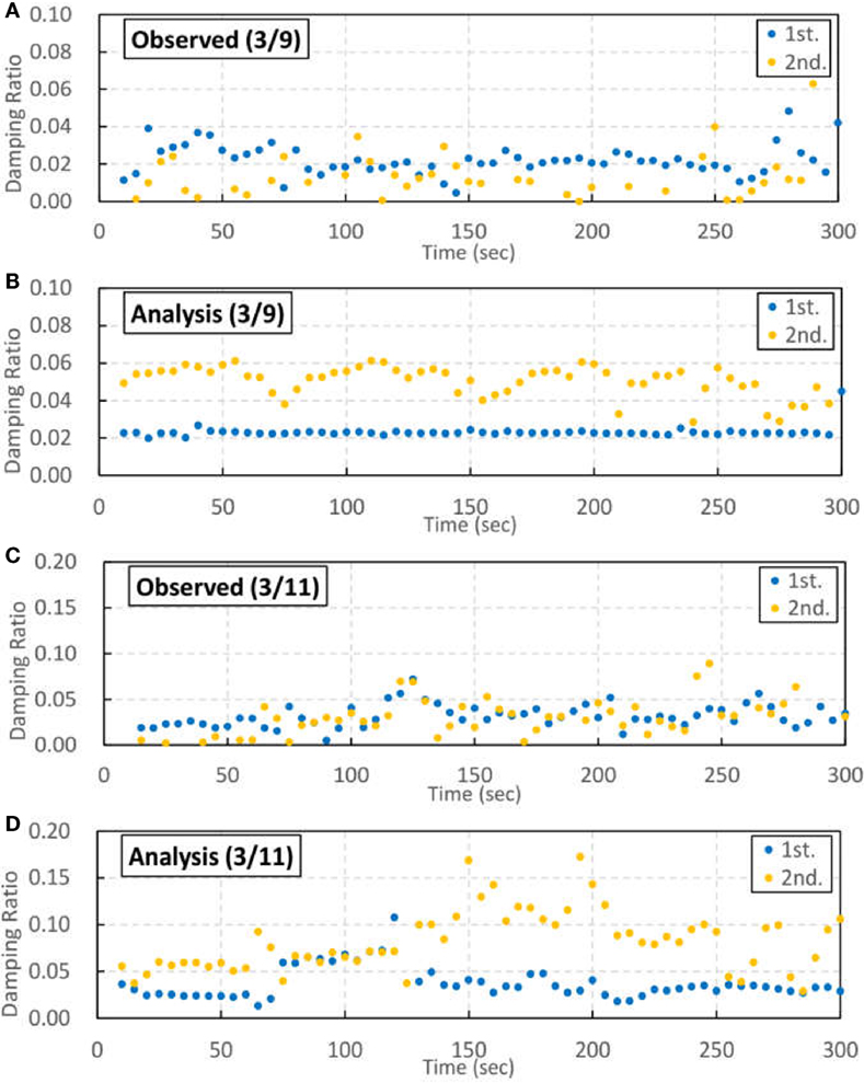
Figure 14. Auto-regressive exogenous analysis results for damping ratio in the N–S direction: (A) change in first and second damping ratios during the 3/9 pre-shock for observed results only, (B) that of analytical result only, (C) that during the 3/11 main shock for observed results only, and (D) that of analytical result only.

A comparison between the first and second damping ratios during the 3/11 main shock from the observed values is shown in Figure 14C. It is evident that the damping ratio increases in accordance with the increased amplitude of the earthquake wave. This is likely the result of the non-linear effect of the building. The ratio of the second mode is similar to the first mode ratio. However, it varies more widely than that of the first mode.

Figure 14D shows a similar comparison for the 3/11 main shock. The first damping ratio from analytical results corresponds to the observed value. However, some differences are apparent between 60 and 120 s. This time period corresponds to when the response increases and non-linearity of the building progresses, as shown in Figure 10A. In Figure 14D, the second damping ratio is greater than the first ratio, most likely because the stiffness-proportional damping model is used in the analysis, in the same way as Figure 14B.

Two cases were also modeled for the 3/9 pre-shock, one with a soil spring (SR), and one without a soil spring (Fixed) in Figure 15. These two cases are compared with respect to the first natural period of the analytical results. It is evident from Figure 15A that the natural period for the SR case is nearly 2.04 s, and nearly 1.94 s for the fixed case (5% difference). This result corresponds to the initial property of 2.035 and the fixed base of 1.940, as shown in Table 4.

FIGURE 15

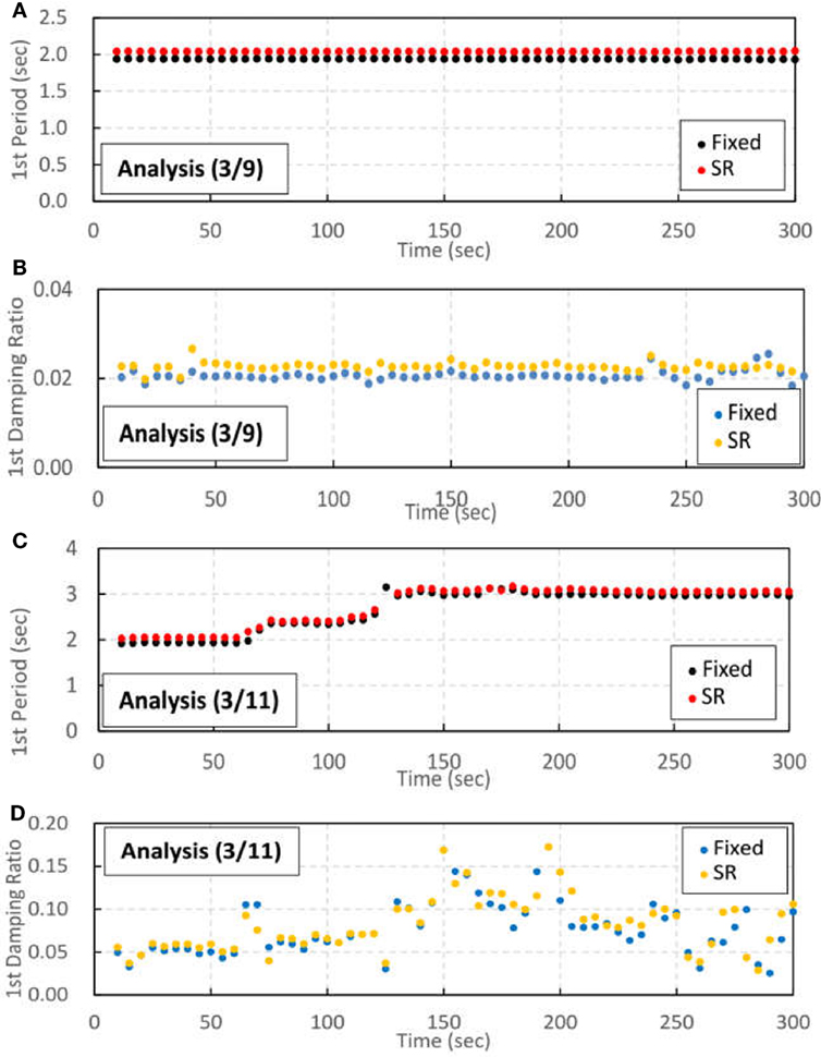
Figure 15. Comparison of analytical results for the “fixed” and “SR” models (N–S direction): (A) first natural periods during the 3/9 pre-shock, (B) first damping ratio during the 3/9 pre-shock, (C) first natural period during the 3/11 main shock, and (D) first damping ratio during the 3/11 main shock.

Similarly, Figure 15B shows a comparison of the first damping ratios from the analytical results of the 3/9 pre-shock. The damping ratio for the SR case is nearly 2.2% and that of the Fixed case is nearly 2.0%, again a difference of 5%. It is considered that the differences in natural period and damping ratio result from differences in response (Figure 12A).

Figures 15C,D show the same comparison between the first natural period and first damping ratio of the 3/11 main shock, respectively. It can be seen that the difference between SR and fixed is smaller than that of the 3/9 main shock. It is considered that the non-linearity of the building increased and the effect of the soil spring decreased, which is consistent with the slight differences in response shown in Figure 12B.

Conclusion

In this study, a lumped-mass system SR model was used to perform seismic response analysis using observational data as input. The first and the second natural periods and damping ratios of both records and analytical results were identified using an ARX model. The main conclusions of this study can be summarized as follows:

(1)  Observational records of the 3/11 main shock at GL show that the shaking level was between Level 1 and Level 2 of the Japanese building code. Ground response analysis shows that the maximum shear strain in the ground was about 0.1% and that the likelihood of liquefaction was low.

(2)  There is little difference between use of a soil spring and an SR spring with initial properties with respect to the 3/11 main shock. This is because the non-linearity of the ground was comparatively small and because of the stiffness of the substructure of the building and diaphragm walls.

(3)  Seismic response analysis, which used input waves generated from observational records at GL, shows that the analytical results correspond well with observed results in the N–S direction, but a slight difference is evident for the E–W direction.

(4)  The stories of the building showed elastic behavior during the 3/9 pre-shock, but exceeded the cracking point and behaved non-linearly during the 3/11 main shock. However, the maximum displacement did not exceed the yield point.

(5)  Based on the observed wave, the natural period of the building increased during the 3/11 main shock. This behavior was generally reproducible in the response analysis. This prolonged natural period results from the non-linearity of the superstructure, while the non-linearity of the ground is negligible.

(6)  Continuous analysis of the 4/11 aftershock involved input of the subject seismic wave after the 3/11 main shock. The results generally correspond well with the observed values, indicating that the effect of the non-linearity of the main shock was retained in the building. This is an important consideration for conducting response evaluation.

(7)  The effect of the soil spring (a rocking spring in particular) was significant during the weak 3/9 pre-shock. Given that the effect of building non-linearity was substantial during the 3/11 main shock, the effect of the soil spring decreased.

(8)  The first and the second natural periods, and damping ratios, were evaluated with an ARX model during vibration. Overall, the response analysis model reliably estimates changes in response of the building to vibrations.

(9)  Although the first and the second damping ratios were similar to the observed results, the second damping ratio was overestimated in the analytical result because of the stiffness damping model.

(10) The effect of the soil spring evaluated by the ARX model shows similar trends to those described earlier for the weak 3/9 pre-shock analysis.

(11) The damping ratio for the building material in the analysis was 2%, which is considered appropriate, while 3% is used generally in Japanese structural design for RC and SRC buildings. Further observational and analytical results are needed to improve estimation of appropriate damping ratios.

Author Notes

Part of this manuscript comes from an English language translation of Nakamura et al. (2013) originally published in Japanese. The copyright of the article published in AIJ Journal of Technology and Design rests with the authors and no further permission is required for the publication of the translated parts.

Author Contributions

NN carried out the theoretical, numerical analysis and supervised the overall work. TK carried out the numerical investigation. HF confirmed the observed data and analysis results.

Conflict of Interest Statement

The authors declare that the research was conducted in the absence of any commercial or financial relationships that could be construed as a potential conflict of interest.

Acknowledgments

The authors wish to acknowledge the support and cooperation of subsidies for the project servicing the architectural standards from the Ministry of Land, Infrastructure, Transport and Tourism. This project was undertaken in cooperation with the technical committee on seismic safety for RC structures under long period ground motions chaired by Dr. H. Shiohara, professor at the University of Tokyo. We thank Warwick Hastie, Ph.D., from Liwen Bianji, Edanz Group China (www.liwenbianji.cn/ac), for editing the English text of a draft of this manuscript.

References

Architectural Institute of Japan (AIJ). (2011). Preliminary Reconnaissance Report on the 2011 off the Pacific Coast of Tohoku [in Japanese]. Tokyo, Japan: AIJ.

Google Scholar

Çelebi, M., Kashima, T., Ghahari, S. F., Abazarsa, F., and Tacirogluc, E. (2016). Responses of a tall building with U.S. code-type instrumentation in Tokyo, Japan, to events before, during, and after the Tohoku Earthquake of 11 March 2011. Earthq. Spectra 32, 497–522. doi: 10.1193/052114EQS071M

CrossRef Full Text | Google Scholar

Hardin, B. O., and Drnevich, V. P. (1972). Shear modulus and damping in soils: design equations and curves. J. Soil Mech. Found. Div. 98, 667–692.

Google Scholar

Ikeda, A., Fujita, K., and Takewaki, I. (2014). Story-wise system identification of shear building using ambient vibration data and ARX model. Earthq. Struct. 7, 1093–1118. doi:10.12989/eas.2014.7.6.1093

CrossRef Full Text | Google Scholar

Ikeda, Y. (2016). An active mass damper designed using ARX models of a building structure. Earthquake Engng Struct. Dyn. 45, 2185–2205. doi:10.1002/eqe.2754

CrossRef Full Text | Google Scholar

Jishin Kougaku Kenkyusho Inc. (2003). Super ALUSH Theoretical Manual. Tokyo, Japan: Jishin kougaku kenkyusho Inc.

Google Scholar

Kawase, H. (2014). Sutdies on the 2011 Off the Pacific Coast of Tohoku Earthquake. Springer.

Google Scholar

Loh, C. H., and Lin, H. M. (1996). Application of off-line and on-line identification techniques to building seismic response data. Earthq. Eng. Struct. Dyn. 25, 269–290. doi:10.1002/(SICI)1096-9845(199603)25:3<269::AID-EQE554>3.0.CO;2-J

CrossRef Full Text | Google Scholar

Nakamura, N., Kashima, H., Kinoshita, T., Ito, S., Miyamoto, Y., Sone, T., et al. (2016). Study on horizontal first mode vibration characteristics of low and middle-rised RC and SRC buildings considering amplitude dependency. J. Struct. Construct. Eng. 81, 471–482. doi:10.3130/aijs.81.471

CrossRef Full Text | Google Scholar

Nakamura, N., Kinoshita, T., Ishikawa, Y., Ota, H., Ikeda, S., Ito, M., et al. (2013). Response analysis of SRC high-rise building during the 2011 off the Pacific coast of Tohoku Earthquake. AIJ J. Technol. Des. 19, 53–58. doi:10.3130/aijt.19.53

CrossRef Full Text | Google Scholar

Okawa, I., Kashima, T., Koyama, S., and Iiba, M. (2013). Recorded responses of building structures during the 2011 Tohoku-Oki earthquake with some implications for design practice. Earthq. Spectra 29, S245–S264. doi:10.1193/1.4000130

CrossRef Full Text | Google Scholar

Safac, E. (1992). Identification of linear structures using deiscrete-time filters. J. Str. Eng. 117, 3064–3085. doi:10.1061/(ASCE)0733-9445(1991)117:10(3064)

CrossRef Full Text | Google Scholar

Saito, T. (1998). System identification of a high-rise building applying multi-input-multi-output ARX model on modal analysis. J. Struct. Construct. Eng. 508, 47–54. doi:10.3130/aijs.63.47_1

CrossRef Full Text | Google Scholar

Schnabel, P. M., Lysmer, J., and Seed, H. B. (1972). SHAKE: A Computer Program for Earthquake Response Analysis of Horizontally Layered Sites, Report No. EERC 72/12. Ph.D. Dissertation, University of California, Berkley.

Google Scholar

Uebayashi, H., Nagano, M., Hida, T., Tanuma, T., Yasui, M., and Sakai, S. (2016). Evaluation of the structural damage of high-rise reinforced concrete buildings using ambient vibrations recorded before and after damage. Earthq. Eng. Struct. Dyn. 45, 213–228. doi:10.1002/eqe.2624

CrossRef Full Text | Google Scholar

USGS. (2016). Magnitude 9.0 – Near the East Coast of HONSHU. Japan. Available at: http://earthquake.usgs.gov/earthquakes/eventpage/official20110311054624120_30#executive

Google Scholar