Sensing of Indoor Air Quality—Characterization of Spatial and Temporal Pollutant Evolution Through Distributed Sensing

Background

Indoor Air Quality

Indoor air pollution presents building occupants with a variety of chronic health risks (Chan et al., 2015). It has consistently been placed by the US Environmental Protection Agency (EPA) as one of the top five risks to environmental public health (US EPA OAR., 2015). Many indoor pollutants have known adverse health effects on humans, ranging from irritation of nasal and mucous membranes to permanent or cancer causing effects (Spengler and Sexton, 1983). Increased levels of CO₂ in indoor air have statistically significant correlations to declines in cognitive performance, even at levels that are deemed acceptable by standards like ASHRAE (Allen et al., 2016). VOCs can cause ear, nose, and throat irritation, and particulate can contribute to lung disease (Kim et al., 2010). Levels of indoor air pollutants can be two to five times as high as outdoor levels, sometimes reaching 100 times as high (US EPA OAR., 2015). This is particularly alarming when we consider that urban populations spend as much as 90% of their time indoors (Spengler and Sexton, 1983). Given the proportion of their time we spend indoors, it is important that we understand what is in the air we breathe.

Contemporary building design and construction practices produce buildings that rely on numerous systems working in tandem 24/7 to deliver the services we expect. HVAC, plumbing, wiring, and finishes deliver comfort and convenience to occupants, but they can also unintentionally degrade indoor environment quality. Air pollution levels indoors are determined by the complex balance between the potency of indoor sources, modes of air penetration through the building envelope, and outdoor air pollution levels. Indoor and outdoor air pollution sources can be categorized several ways; they may be mobile or static, and with stochastic or continuous pollution signals. Additionally, static sources may be point sources or zonal polluters. Each type of source poses a unique challenge to the mediation of pollution in indoor air, and similarly a unique challenge to measuring it. Figure 1 provides some examples of where different sources fall into such a categorization scheme.

FIGURE 1

Figure 1. Pertinent to the sensing of indoor air quality is whether a particular source pollutes continuously or stochastically, and whether a source is mobile or static. Common sources of indoor air pollution are categorized as examples.

There are many sources of air pollution indoors. The breathing of humans and pets, as well as combustion, contribute water vapor and CO₂. Volatile organic compounds (VOCs) are released by building finishes and cleaning products. Plants, animals, humans, and printers all contribute particulate to indoor air, though they are only a subset of a large number particulate polluters (Fisk and de Almeida, 1998). Currently, we have the technological capability to better understand pollutant levels in buildings with inexpensive sensor networks, and more easily attempt to spatially identify both static and mobile sources of pollution. By analyzing variation across time and space, we believe it is also possible to determine if they are continuous or stochastic polluters.

Current Ventilation Control Challenges

With the ongoing push to tighten up the building envelope, modern buildings often rely exclusively on mechanical ventilation to dilute indoor pollutants to acceptable levels. Ventilation systems are commonly operated on simple air exchange rate standards and rules of thumb, and without information about actual air pollution levels. These conditions necessitate a greater understanding of the dynamics of air quality in buildings, and how these relate to the ever-changing state of air quality outside of them.

Air exchange rates are usually mandated as functions of the maximum number of occupants and the floor area, in addition to maximum acceptable levels of pollutants (ASHRAE, 2009). As actual pollutant levels are rarely monitored by HVAC systems, standard practice is to simply ensure a room volume is ventilated at a constant, pre-calculated rate. With fixed airflow rates, over-ventilation is a serious energy concern (ASHRAE, 2009). The Federation of European Heating, Ventilation and Air Conditioning Association's REHVA Guidebook No. 6 provides quantification of the effect of increased ventilation rates on occupant productivity in offices (Wargocki, 2006). In response to these figures, a Dutch study found that to increase productivity and occupant satisfaction with air quality, it is more effective to remove indoor air polluters than it is to increase ventilation rates (Kurvers and Leyten, 2010). This result supports the need for developing iAQ monitoring systems that are able to detect the location of indoor air pollution sources, such that sources can be removed rather being dealt with by increasing ventilation rates, or not dealt with at all.

A natural evolution of ventilation control logic is to use timer-controlled setbacks, programmed according to use patterns. This is often done for office buildings with typical working hours. Setbacks acknowledge that many of the most aggressive degraders of indoor air—like people—are mobile and their presence varies at quasi-regular intervals. Energy consumption is reduced by turning ventilation systems down or off for several hours at a time. The fundamental weakness of this technique is that it does not account for occupation of spaces outside of preprogrammed schedules, and requires manual reprogramming for changes in timing. Some consumer HVAC controls, like the Nest Learning Thermostat^®, try to address this issue by making schedule detection an intrinsic part of the control logic, using motion sensors to learn the pattern of space usage (Nest Labs, 2017).

Sensor Based Demand Controlled Ventilation (SBDCV)

Sensor based demand controlled ventilation adds a feedback layer to scheduled ventilation control. This technique commonly uses feedback from CO₂ sensors to modulate flow rates. As CO₂ levels are increased by exhalation, it can be used as a proxy for measuring occupancy. Still, ensuring low CO₂ levels alone does not guarantee indoor air quality (iAQ). There is little correlation between CO₂ and traffic related pollutants for instance (Chatzidiakou et al., 2015). When we look holistically at iAQ, there is likely a very poor correlation between the occupancy artifacts (CO₂) and the amount of other pollutants, like VOCs emitted by static building materials. Also of major concern is that the standards that dictate target levels of CO₂ in buildings have recently been proven insufficient to guarantee well-being (Allen et al., 2016). Passive infrared (PIR) motion detectors are used in some buildings for ventilation control, but these systems are fraught with issues. PIR motion detecting is unable to detect static people, and can turn off ventilation when people are static long enough. Particulate sensors have been used in high concentration spaces, like smoking lounges, but high quality particulate sensors have historically been expensive (Fisk and de Almeida, 1998), though drops in prices have made them more accessible. Moisture sensing is used in some residential ventilation controls, but SBDCV systems are commonly univariate.

The issue persists that ventilation rates determined by the value of a single iAQ metric disregards the complexity of the factors that determine iAQ. When SBDCV is unable to accurately characterize pollution levels, dilution will be insufficient, and a gradual increase in pollution levels can happen over time (White et al., 1987). Common across applications of SBDCV is the assumption that outdoor air is “cleaner” than indoor air. While this may be generally true, building systems never empirically confirm this, and do not possess the faculties to. When a stochastic pollution event happens, inside or outside, building controls are usually unaware and are incapable of increasing preprogrammed ventilation rates in response to the degradation of indoor air.

We propose that future SBDVC should look holistically at indoor environment quality, supplying the necessary amount of outdoor air to ensure low enough levels of all iAQ metrics, not just one or two. Further, systems should be able to detect when air quality is satisfactory, such that ventilation can be decreased, or turned off entirely, and the associated energy savings can be reaped. The purpose of the on-going development of our indoor environment quality (iEQ) sensor network is to determine whether a holistic and spatially explicit characterization of iAQ can be accomplished, with hardware of a sufficiently low-cost that SBDVC could conceivably be employed in many kinds of buildings, not just expensive ones.

Existing Tools

Indoor air quality is often experimentally verified with handheld equipment. Devices like the TSI Q-Trak 7575, used by Allen et al. in his seminal study on the effects of CO₂ on cognition (Allen et al., 2016), can cost more than $3,000 USD. Professional grade equipment like this can be prohibitively expensive when looking at the number of devices needed to address questions of spatial and temporal evolution. Even at this price point, handheld devices lack connectivity, making any kind of real-time monitoring impossible. The explosion of IoT devices has brought a few iAQ measuring devices to the consumer market, but these are limited in the range of iAQ parameters they measure. The Netatmo weather station also used by Allen et al. costs $100 USD per node and can only measure temperature, humidity, and CO₂. To make iAQ evolution monitoring possible at a high temporal and spatial resolution, we need to develop new tools.

The Need for Distributed Sensing

Until now, deployments of iAQ sensing equipment in buildings have primarily studied how the chemical concentrations that sensors are exposed to change over time. “Efforts to access health risks associated with indoor pollution are limited by insufficient information about the number of people exposed, the pattern and severity of their exposures, and the health consequences of exposures” (Spengler and Sexton, 1983). By allowing researchers to monitor the spatial and temporal evolution of indoor air pollutants, we hypothesize that iEQ sensor networks like ours have the potential to provide the kinds of information Spengler and Sexton are referring to. Until now, research on building low-cost multivariate iAQ sensor networks have been primarily to prove that the technological feat of collecting data by such a system is possible (Kim et al., 2010; Abraham and Li, 2016), using data gathered to feed models (Jin et al., 2017), or were of a low spatial resolution (Blondeau et al., 2005). Researchers have built and calibrated low-cost, networked, sensor nodes but there is limited literature focused on the deployment of these technologies to study iAQ spatially in buildings. We hope to address the lack of spatially oriented iEQ analysis in buildings by deploying sensor nodes, measuring many parameters, in different buildings to study the evolution of indoor pollution through time and space.

Existing Distributed iAQ Sensor Systems

While CO₂ sensing has been available in certain demand controlled ventilation systems for a few decades (Emmerich and Persily, 1997; Fisk and de Almeida, 1998), they don't provide a comprehensive view of indoor air. The building management systems (BMS) that hold the data often have a low temporal resolution, insufficient storage capacity, and a steep learning curve; making iAQ insights difficult to gather, and nearly impossible to acquire in real-time, or near real-time. In response to this, researchers have developed microcontroller based iAQ nodes capable of addressing many of these issues.

In 2010, Kim et al. published a paper describing their attempt to address the need for distributed iAQ sensing (Kim et al., 2010). Their battery powered nodes could measure CO₂, CO, VOC, O₃, and particulate, and their network infrastructure was built around the ZigBee transceiver for its strong energy consumption to range ratio. Minimizing unit costs were stated to be the driving design consideration. Their platform was thoughtfully executed, though their network architecture had a level of complexity necessitated by their use of ZigBee. Their architecture required the transceivers on each node to communicate through gateways to a base station that was physically connected to a PC.

In 2013, a paper published in Medical Engineering and Physics by Yu et al. details their iAQ wireless sensor network (WSN) nodes and network typology (Yu et al., 2013). Using the ZigBee protocols, Yu et al. built nodes that could measure temperature, humidity, and CO₂ concentrations, and were able to remove the base station and tethered computer from Kim et al.'s network. This new strategy could jump communication from multiple locations to the Internet, where data was aggregated and stored on an application server off-site. While they could measure fewer metrics than Kim et al., their infrastructure was less complex and more scalable.

In 2016, the International Journal of Information Networks published a detailed account of the development of an iAQ sensor network by Abraham and Li (2016). Their network is structured similarly to Yu et al.'s but their nodes support more iAQ parameters, thanks in part to their inclusion of an open source microcontroller. Their nodes support CO₂, VOC, O₃, temperature, and humidity sensors. The addition of a dedicated microcontroller for data acquisition (DAq) likely doubles the unit cost of the DAq and communications components on each node.

A recent paper (Pantelic et al., 2018), describes the development and application of a sensor network work that breaks away from the ZigBee protocol norm. In its place, the microcontroller platform Particle.io is utilized. This platform leverages a combined microcontroller and WiFi communication chip to deliver processing and communication in a very cost effective package. This typology removes the need for gateways and base Stations that are required by the ZigBee protocol. In a first iteration, their nodes host NO₂, CO₂, CO, O₃, VOC, Particulate, temperature and humidity, curating out CO, O₃, NO₂ in the second version so only highly calibratable sensors would be used. While the cost of DAq and communications in their nodes is about half that of Abraham and Xinrong's, it is at the expense of greater power consumption.

In the following section, we describe the development of a similar network architecture to Rysanek and Pantelic. On our nodes we embrace low-cost, less easily calibrated sensors, as a tool to spatially identify points sources of pollution, and track their evolution in relative terms though space and time.

Methods

Infrastructure

To be able to study the evolution of air quality in and around buildings, with a high temporal and spatial resolution, it was imperative that we developed an underlying infrastructure that was flexible and scalable. We used a wide variety of existing sensor components and assembled them around the WiFi enabled microcontroller platform from Particle.io. Data can be published to a Server-Sent Event (SSE) stream, but is limited to a single publish per controller per second. To extract 7 iEQ data points per node per second, we developed a firmware side encoding structure. To capture data, we wrote software to monitor the SSE stream, decode incoming packets, and logged to an instance of the open source InfluxDB database. Data is graphed in real-time by the open-source software Grafana, allowing us to catch errors and monitor readings. This infrastructure and data flow enables us to carry out many experiments concurrently, and monitor results in real time (Figure 2). During the period of highest demand on the system, it supported data acquisition and visualization from 60 nodes, measuring 100 parameters.

FIGURE 2

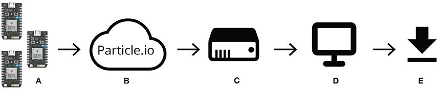
Figure 2. Data collection system overview. Data from an arbitrary number of microcontrollers (A) is published to Particle.io's Cloud API (B). Our server (C) scrapes the data, and stores it in an instance of InfluxDB, where client (D) can view the data in Grafana and download for analysis (E).

Nodes

The microcontrollers used afford great flexibility in the kinds of sensors we can record data from. Each node is built from a combination of the sensors in Table 1. We grouped sensors onto one of two nodes, based on power requirements and cost. We milled circuit boards to increase the robustness of deployed nodes over breadboards, and 3D printed cases to mitigate sensitivity to high velocity airflow in ducts. We produced 6 duplicates of each node configuration, a dozen nodes in total (Figure 3). The first node configuration included a factory calibrated high sensitivity CO₂ sensor, that returns digital values in parts per million. The second configuration had Ozone, formaldehyde, nitrogen dioxide, VOCs, humidity, and temperature. Except for temperature and humidity which are digital, these sensors return voltages which are read into the microcontroller with a resolution of 4,096 points.

TABLE 1

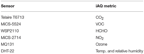
Table 1. All sensors used in node configurations.

FIGURE 3

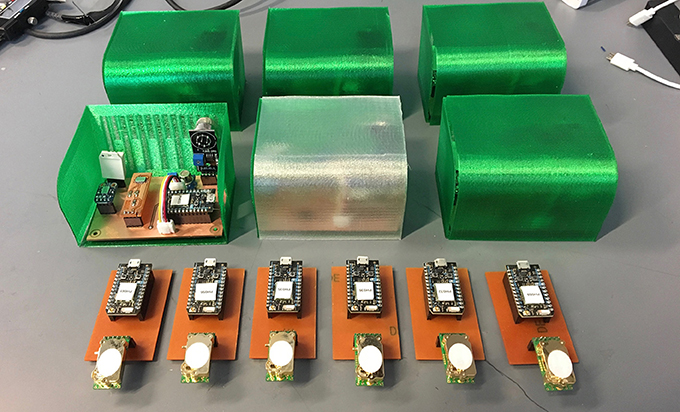
Figure 3. The six multi-iEQ parameter nodes, in their convection blocking enclosures, and six carbon dioxide nodes deployed to buildings on Princeton University's Campus.

Comparative Calibration

While the low-cost of the sensors selected make large scale deployments possible, they do require calibration. Many of the most common instrument calibration techniques and associated literature have been written or developed for absolute calibration (Osborne, 1991). Absolute calibration determines the calibration curve of a device whose measurements deviate from true values by an unknown amount, using the measurements of an instrument with known or negligible error. With these two data sets one may use linear regression—referred to as Eisenhart's Classical Estimator (Osborne, 1991) in the context of comparative calibration—to determine the calibration curve by considering the regression of Y on X (Shukla, 1972). Where Y represents the measurements made with the device to be calibrated, and X represents the measurements of the device whose readings are assumed to be the true values. Finding the slope (β₁) and Y intercept (β₀) of the line of best fit for Y | X will produce the estimator.

$E\left(Y|X=x\right)={\beta }_0+{\beta }_{1}x\left(1\right)$

Equation 1: Eisenhart's Classical Estimator.

We did not have absolutely calibrated instruments to calibrate our multi-parameter nodes with. In lieu of a set of true values, X, we created a substitute to calibrate the individual sensors against. While it is common in this scenario to choose one measuring device, and set it as the standard to calibrate the other measuring devices against, we elected to generate a new series that better accounted for the spread of measurements at any specific time. We started by placing the 6 multi-parameter nodes and 6 single parameter nodes on a table in the lab where they would not be disturbed. The configuration was like the arrangement in Figure 3, where all the sensors fit into a roughly 14″ × 14″ space, and would be exposed to the same changing conditions over time. We let the sensors record continuously for 3 days. We fed the resulting data to a python script that employed Eisenhart's Classical Estimator to generate calibration functions for each raw signal. For each iEQ parameter being recorded, a median signal was generated from the 6 raw signals. Each raw signal was then regressed with the median signal, using the polyfit function of Python's Numpy library. The function generates the line of best fit by minimizing the squared error, the operation used is found in Equation (2).

$\begin{array}{ll}E={\displaystyle \sum _{j=0}^k}{|p(x_j)-j_j|}^2& \left(2\right)\end{array}$

Equation 2: The statistical operation employed by Python polyfit function. Used for calibrating all sensor signals used in our experiments.

Units

The dissimilar nature of signals from specific types of low-cost gas sensors make using uniform units problematic. Some sensors are digital, and output values are within preprogrammed ranges. Some sensors are analog, and responses are translated from voltage to digital values by the microcontroller's analog-digital-converter (ADC). In some cases, we do not know the possible voltage range of analog signals, and by extension the range in possible ADC readings. In other cases, we know the range of voltages, and have been provided a translation function by the manufacturer. Due to these differences, it is not possible to convert all outputs to the same units for the comparison. As such, we will generally present data in generic “units.” We will be comparing signals of like sensors whose magnitudes, in units, change synchronously to changing chemical concentrations. This will be the case except when it is possible to use the actual units recorded; like when we are discussing ppm CO₂, or variation in ADC readings of the same model of sensor.

Deployment Locations

We deployed our iEQ nodes in two pilot experiments on Princeton University's campus. The first is to a large singe-volume fabrication building, the Embodied Computation Lab (ECL). The second is to a combination office and research lab space, the Andlinger Center for Energy and the Environment (ACEE).

In the deployment to the ECL, we placed sensor nodes at three points in the ventilation supply chain: the Fresh Air duct, the Supply diffuser, and across the space on a Flammable materials cabinet. Qualitatively, we hoped this selection of spatial positions would give us an understanding of the proportional increase/decrease of iAQ parameters as outdoor air entered the building, was affected by the air handler, and then diffused across the large assembly space, to the farthest point from the supply vent. In addition to being on the farthest wall from the supply vent, the cabinet was specifically chosen because we suspected it to be a major contributor of pollution to the interior environment. Presumably, this position would be representative of the worst-case scenario of air quality in the space. The nodes were left running for an 8-day period.

For the second experiment, we moved to the ACEE building, where we scaled up the deployment size to 6 points in the ventilation supply chain. For this deployment, we placed 3 sensors in the air handling unit; one at the fresh air intake, one after the filter, and one after the heating and cooling coils. Additionally, we placed 3 in an open-plan graduate student office, serviced by the air handler. We placed sensors at the more populated west side of the room, as well as at the less populated east side of the room. A sixth position was selected in front of the air return grill in the plenum of the space.

Results

Calibration

Using the outlined comparative calibration methodology, we significantly increased the relative precision of the calibrated sensor signals. For the 7 iEQ metrics being calibrated, we saw the average range in sensor responses decrease by 89.1%, and an 89.2% decrease in standard deviation. More specifically, the calibration methodology produced the greatest reduction in range of signals for the ozone sensors, with a 96.5% reduction in range. Similarly, the average standard deviation during the calibration experiment was reduced by 96.1%. The calibration methodology produced the lowest reduction in range for the signals produced by the NO2 sensors, where it was reduced by 75.7% on average, with a 76.7% reduction in standard deviation. The complete results of the calibration of sensor outputs are found in Table 2.

TABLE 2

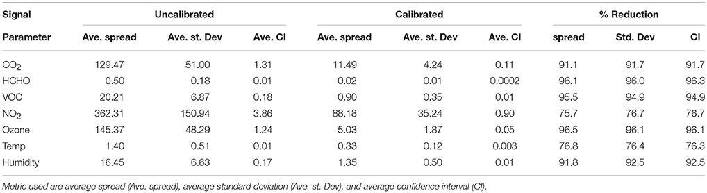
Table 2. Summary statistics from the uncalibrated and calibrated sensor signals, during the calibration experiment.

Our calibration methodology reduced the spread and standard deviation of the digital CO₂ sensor signals by 91%. The other gas sensors used were effectively comparatively calibrated to the precision needed for relational observations, as elaborated in the next section, but require further experimentation in a lab to correlate response curves to absolute ppm accuracy.

VOCs in the Embodied Computation Lab Building

After assessing the 7 iEQ parameters measured, the parameter with the clearest trends was VOC concentrations, shown in Figure 4. Periods where the sensor lost connectivity were removed for legibility. We plot first the raw ADC response for each of the three locations at the supply, the diffusor in the space, and in the space near the flammables cabinet. We then plot the difference between each of these points.

FIGURE 4

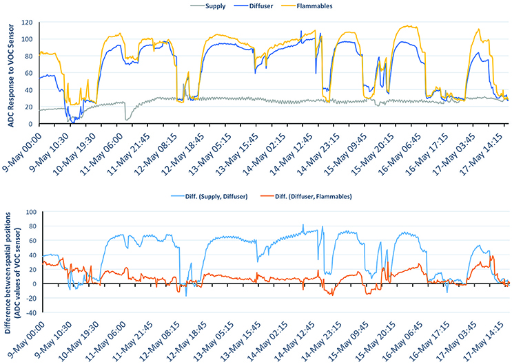
Figure 4. The calibrated VOC sensor signals recorded in the Supply air duct, at the supply air Diffuser and at Flammables cabinet in the Embodied Computation Lab (top). The difference between the calibrated ADC readings of the VOC sensors at the Supply and the Diffuser, and between the Diffuser and Flammables cabinet (bottom).

There are clear points where the buildings doors are open and the fresh air is mixing causing similar values at all sensors, and clear points where the VOC's rise in the room, both at the diffusor and near the flammables. There is a dramatic increase in VOC concentrations between when fresh air is brought into the building's ventilation system and when it mixes with the air in the main volume, on average a 177% increase. There is a much less dramatic increase in the VOC concentrations of the air between the point where fresh air is mixed with existing air, and a probable point source of VOCs, the flammables cabinet located about 50 feet away. This difference is only a 33.7% increase on average. Figure 4 shows that air with a low VOC content is consistently being brought into the ventilation system from outside. However, that fresh air becomes polluted with VOCs almost immediately after exiting the diffusor, suggesting a high volatility and diffusivity of the pollutant in the air volume.

Multi-Parameter iEQ Monitoring at ACEE Building

Figure 5 shows the VOC signals from 6 comparatively calibrated sensors. The calibration of these sensors yielded a comparative precision of ±0.7 units (2σ). We found that the graduate student space consistently had VOC levels higher at desk height (PhD East and PhD West) than the buildings fresh air stream. The difference between the mean desk height VOC reading in the graduate space and the fresh air stream was a 7.5% increase on average (1.3 units). The post filter air consistently had the lowest VOC levels in the supply chain; on average 40.4% lower (7.2 units) than the fresh air stream. Between the post coil section of the air handler and the desks of the graduate room, an average increase of 56.1% in VOC levels (6.4 units) occurred. With regard to the spatial evolution of pollutants across the entire ventilation supply chain, this dataset suggests that the air handling unit's filter consistently lowers the VOC content in the air. By the time the air passes the heating and cooling coils in the air handler VOC levels rise slightly. Supply air in the graduate space is provided at ceiling level, by desk height the air consistently sees the highest levels of VOCs in the supply chain. While the difference between the west (more populous), and east (less populous) part of the graduate student area was close to the 2σ (two standard deviation) margin of error for calibration, there does appear to be a consistently higher VOC concentration in the west part of the room from the 16th of August to the 20th. The air in the plenum (in front of the exhaust duct) appears to have roughly the same VOC content as the fresh air stream of the building.

FIGURE 5

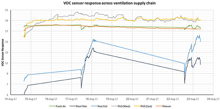
Figure 5. The comparatively calibrated signals of 6 VOC sensors across the ACEE ventilation supply chain.

In Figures 6, 7 we investigate the inter-parameter iEQ relationships in the PhD West (more populous) side of the graduate space, facilitated by the 7 low-cost sensors included in each cluster. The 7th parameter, ozone, has been omitted from the graph and subsequent analyses; a bug in the firmware rendered the values recorded unrepresentative of the true ozone concentrations in the space. Narrowing the focus of the probe to one spatial location allows us to investigate questions of periodicity, and the correlation of periodicity between parameters. We produced 24-point curves, where each point represents the average hourly value over the 8-day experimental period. Several of these graphs are found in Figure 7. For NO₂ and VOC levels, the highest concentration appears at 6 a.m. and 5 a.m., respectively. This is likely an indication that the concentration of these chemicals builds up over the course of the night, when the air is being replaced at a reduced rate due to setbacks, and drop away over the course of the day, once the ventilation systems switches to its day turnover rates at 6 a.m. The correlation of these two parameters are studied in Figure 7A, where the average hourly VOC values are regressed against the average hourly NO₂ values. The same is done for HCHO and relative humidity (RH) in Figure 7B. The resulting R² value for VOC and NO₂ is 0.475, indicating a likelihood of being similarly influenced by setback controls. However, for HCHO and RH the R² value is 0.051, indicating the unlikeliness of a common influence on those parameters.

FIGURE 6

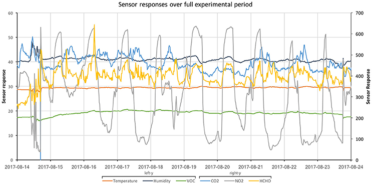
Figure 6. All iEQ parameters measured at the west location in the PhD student office (PhD West) over the full duration of the ACEE experiment (Except ozone).

FIGURE 7

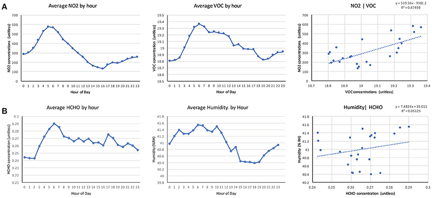
Figure 7. Average hourly values from the NO₂ and VOC sensors at the PhD West location (A), demonstrating an R² of 0.47, indicating the likelihood of a common influence. Average hourly values from the HCHO and relative humidity sensors (B), R² of 0.05, indicates an unlikely common influence.

To demonstrate the ability of our low-cost iAQ sensor network to identify more complex pollutant evolution drivers, we investigated CO₂ levels in the graduate student office (Figure 8). Predictably, we found that they directly correlated with occupancy in the room. The highest levels of the day occurred at 11 a.m. (510 ppm), followed by a decline in levels while occupants left for lunch. We saw a mild increase in CO₂ after the return of occupants from lunch. The lowest CO₂ levels of the day were observed between 7 p.m. and 8 p.m., after which they begin to rise, corresponding to the ventilation system entering night mode. This reiterates the trends seen in the gradual rise of NO₂ and VOCs in the space overnight. The plenum—which feeds the exhaust air duct—showed consistently higher CO₂ levels than the desk height sensors.

FIGURE 8

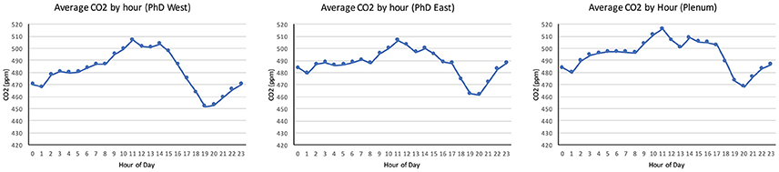
Figure 8. Average hourly CO₂ levels in the graduate office of ACEE, for the whole experimental period.

Discussion

Significance of Results

The initial results from the ECL space characterize a ventilation system that is consistently unable to dilute indoor concentrations of VOCs. The ECL deployment showed through the analysis of VOC levels over time, and through space, that low-cost distributed sensor clusters can be used to identify where pollutants are being introduced in a simple ventilation supply chain, even at a low spatial resolution. The investigation of iAQ in the ECL was an initial investigation, and the broader deployment used at the ACEE building can easily be used to refine the anlaysis in future work.

We were able to derive meaningful insights about the spatial and temporal evolution of air quality in ACEE. Focusing on the spatial evolution of iEQ, the data describes a building with internally driven VOC concentrations. More specifically, VOC levels in ACEE were found to be highest at desk height in the office. Finer resolution still, we found that the more occupied part of the office consistently had higher VOC levels than the less occupied part. With this spatial resolution of data, we can begin to demonstrate evidence of a correlation between occupancy and the evolution of VOC levels, which is useful then to justify investigation into the exact mechanisms that cause VOC levels to be affected by occupancy. The BMS system of ACEE has no capacity to measure VOCs, so it would require at least as many expensive unconnected handheld sensors as spatial positions in our experiment—with operators recording the data—to arrive at the same conclusion. The data provided by our multi-parameter nodes also describe a building with NO₂ and VOC concentrations driven by ventilation set-backs, and CO₂ concentrations driven by both occupants and ventilation set-backs. Again, the BMS system of ACEE has no capacity for measuring NO₂ or CO₂. To arrive at the same conclusions about periodicity and correlation, we would have had to purchase another set of expensive gas sensors. If it were possible to source the necessary handheld sensors with data logging capability, independent of the associated expense, there is still the issue of data aggregation and time-stamp synchronization. In our Internet of Things (IoT) based solution, aggregation and synchronization of data become standard parts of the way the system works, rather than another task a researcher must do before knowledge can be generated from data streams. A distributed, IoT based system of low-cost iEQ sensors dramatically lowers the barrier to collect data on the spatial and temporal evolution of iEQ. We believe that this kind of system opens the opportunity for a much larger base of researchers to study this topic than have historically, and will empower that body of researchers to study more buildings, more quickly, and with less resources than traditional methods.

Infrastructure and Nodes

When trying to spatially and temporally evaluate the evolution of iEQ parameters, the flexibility and ease of hardware revision afforded by cloud connected microcontrollers creates important new opportunities for deployment. The ability to tweak firmware wirelessly is of great advantage when air quality is being monitored in places that are not easily accessible. This proved valuable in the ductwork of ACEE and the ECL. Likewise, when many devices have been deployed through a space, all firmware revisions can be handled remotely, removing the need to collect and redeploy sensors, and minimizing the time spent on-site. After catching the ozone sensor bug mentioned in section VOCs in the Embodied Computation Lab Building, all 6 of the affected nodes were quickly reprogrammed from our lab. The built-in Wi-Fi radio makes deployments plug-and-play at most locations on campus. Without the need for additional infrastructure, costs were kept down; allowing us to buy more sensors and build more nodes.

Particle's cloud services limit each microcontroller to one data publish per second. We wrote a simple encoding structure that we used to publish around 10 sensor readings, per node, per second. This made the maximum temporal resolution—every second—independent of the number of sensors on each node, invaluable as the number of sensors per node grew. This temporal resolution is much higher than that of the BMS system in the test buildings (~1 reading per 2 min). The primary limitation of Particle.io's infrastructure, that published data is not stored, was overcome with relative ease by writing an aggregation and archiving script. To this end InfluxDB proved to be a strong choice for its time-series functionality, making querying archives simple, and connectivity to graphing software like Grafana low-effort. Being open source was very much in line with our desire to keep costs as low as possible. Real-time visualization proved useful for providing real-time feedback about the conditions in the test buildings, and was very helpful for detecting circuitry and connectivity issues.

We built sensor nodes at a cost that was consistently an order of magnitude less expensive than handheld iAQ measuring equipment, and less expensive than consumer iAQ like Netatmo™. Distributing sensors across multiple nodes was a helpful design choice, prohibiting hardware failure of one node from stopping all data collection at a particular location, because they were physically on different circuits.

We endeavored to understand and develop the techniques to describe the evolution of air quality from intake, through building systems, and into occupied spaces, using data from low-cost iEQ sensors. The deployment to the ECL had an additional position to the three previously discussed. The 4th position was in the exhaust air duct, which we chose to give a more complete cross section of the evolution of air quality in the space. Wi-Fi connectivity proved too problematic to maintain in that part of the ventilation system, and we experienced hardware failure of one of the two nodes at that location. We tried in vain to improve connectivity in the duct by adding an external antenna. The node that failed was one of our prototype bread boarded nodes and a short circuit destroyed it. This confirmed it was necessary to use only milled circuit boards for all our deployments from then onwards.

In the ACEE building, we designed an experiment that would increase the complexity and completeness of the ventilation supply chain cross-section being studied. Three of our six spatial positions were in an office, and availability of power outlets let us run the nodes over the full experimental period. For the other three, which were placed in the office's air handling unit, wired power could not be delivered, and we were limited to collecting data for the duration allowed by lithium-ion batteries. Our 10 ampere hour batteries lasted about 20 h per charge, and we replaced them three times. The air handler is pressurized, and we required the assistance of Princeton Facilities to shut it down before entering the unit. This precluded us from swapping batteries more often, and speaks the necessity of working closely with the test building's owner, operator, or managers for this kind of research.

Calibration

For the purposes of our immediate research, we desired to test the ability of low-cost hardware to monitor the spatial and temporal evolution of indoor air pollutants. In this context, we believe it was more valuable to have many sensors, relatively calibrated, than it was to have a few absolutely calibrated sensors. The makers of many low-cost iAQ sensors leave calibration to the user, so it would require lab testing to determine response curves to exact levels of gases. We theorized it would be possible to spatially identify pollution sources in a ventilation supply chain using low-cost iEQ sensors. However, since absolute values of the iEQ parameters measured by these sensors are not known, it is especially important to have well-correlated responses from like sensors. To this end, we statistically synchronized the outputs of like sensors as closely as possible. Looking at the difference between the readings of sensors measuring the same conditions, we found some sensors had offset error and some also had gain error, necessitating comparative calibration. Though much less literature is available discussing comparative calibration techniques than absolute calibration techniques (Osborne, 1991), we saw a strong improvement in relative precision after applying our linear calibration functions to the sensor signals. To ensure the time/expense of calibrating large numbers of sensor kits was kept minimal, a python script was written to automate this process of finding the calibration function of each sensor. The time and expense required to obtain a dataset that can be used to absolutely calibrate low-cost sensors is prohibitive in some cases, and runs counter to the desire to use low-cost equipment.

Conclusions

We have developed a low-cost distributed sensor system for studying the spatial and temporal evolution of iAQ parameters. Most of the low-cost sensors used did not record at the accuracy of ppm/ppb, so to maximize the usefulness of data we developed an effective comparative calibration technique which was used to quickly, and with no associated cost, synchronize sensor outputs. After cross-calibrating the 7 iAQ signals from each of the 6 nodes, our methodology decreased the range between signals from different nodes by 89.1% on average. The standard deviation in these signals also decreased by 89.2% on average.

The ECL deployment characterized a building where the evolution of VOC levels was internally driven, and illustrated that low-cost distributed sensor clusters can be used to identify where pollutants are being introduced in a simple ventilation supply chain. The ACEE deployment increased the spatial resolution of VOC monitoring, and found variation between all spatial positions. The variation again described a building with internally driven VOC evolution. Having a spatial resolution Finer than the scale of a room, we detected a trend toward higher VOC levels where more people are present. This deployment also allowed us probe periodicity in iEQ evolution, which correlated to occupancy and HVAC set-backs.

We demonstrate through deployments on Princeton's campus that low-cost, IoT based, iEQ sensing systems have the capacity to detect spatial and temporal evolution of indoor environment quality, making this kind of research more accessible. We believe this kind of research will help close the knowledge gap of how exterior and interior air quality are dynamically linked.

Future Work

Future work will include node refinement, larger deployments, and further engagement with building managers as the research serves as an important opportunity for using the campus as a living laboratory, bringing research and practice together. We have begun to purchase high-cost, factory calibrated gas sensors, to comparatively calibrate our low-cost sensors to. Following this, we plan to further investigate new modes of calibration and refine our workflow to quickly and easily calibrate large numbers of sensors. These two steps will add the dimension of severity of exposure to indoor pollutants to the dimensions of spatial and temporal evolution. As our deployments increase in scale, we also plan to broaden the iEQ parameters measured to include metrics like carbon monoxide, and particulate (pm 2.5–10). We may also include parameters of thermal, visual, and acoustic comfort as well. Further development on the nodes will involve the fabrication of weather resistant enclosures and the addition of larger batteries, such that nodes can be used more reliably indoors and out. With these new node designs, we will investigate the full evolution of chemical concentrations from the outside of buildings inwards, and investigate the ability of HVAC systems to dilute or remove pollutants once they have entered the building envelope. Our long-term goal is to generate a data set capable of illuminating how effectively different ventilation systems and schemas deliver health and well-being promoting environments through the protection of iAQ.

Author Contributions

JC: hardware, software, infrastructure development, research and author of paper; FM: hardware development, experimental design, research, author of paper.

Funding

Funding awarded by Campus As A Lab, Office of Sustainability, Princeton University.

Conflict of Interest Statement

The authors declare that the research was conducted in the absence of any commercial or financial relationships that could be construed as a potential conflict of interest.

Acknowledgments

This work was supported by the Andlinger Center for Energy and the Environment, and the School of Architecture at Princeton University. This study was made possible by funds from Campus as a Lab, which is supported by the Office of the Dean for Research, the Princeton Environmental Institute, the Andlinger Center for Energy and the Environment, the High Meadows Foundation Sustainability Fund, the Office of the Dean of the College and Facilities. This study was funded in part by the US National Science Foundation's Sustainability Research Network Cooperative Agreement # 1444758. This work builds upon the precedents put forth by Jovan Pantelic, Adam Rysanek, Clayton Miller, Yuzhen Peng and Arno Schlüter. The ongoing support and guidance of Eric Teitelbaum, and the daily assistance of Justin Hinson were invaluable to the timely execution of the project. We would also like to specifically thank Princeton Facilities for their time, accommodation and cooperation throughout the testing and data collection phases of the project.

References

Abraham, S., and Li, X. (2016). Design of a low-cost wireless indoor air quality sensor network system. Int. J. Wireless Inf. Netw. 23, 57–65. doi: 10.1007/s10776-016-0299-y

CrossRef Full Text | Google Scholar

Allen, J. G., MacNaughton, P., Satish, U., Santanam, S., Vallarino, J., and Spengler, J. D. (2016). Associations of cognitive function scores with carbon dioxide, ventilation, and volatile organic compound exposures in office workers: a controlled exposure study of green and conventional office environments. Environ. Health Perspect. 124:805. doi: 10.1289/ehp.1510037

PubMed Abstract | CrossRef Full Text | Google Scholar

ASHRAE. (2009). Indoor Air Quality Guide: Best Practices for Design, Construction, and Commissioning. Atlanta, GA: American Society of Heating, Refrigerating and Air-Conditioning Engineers.

Blondeau, P., Iordache, V., Poupard, O., Genin, D., and Allard, F. (2005). Relationship between outdoor and indoor air quality in eight french schools. Indoor Air 15, 2–12. doi: 10.1111/j.1600-0668.2004.00263.x

PubMed Abstract | CrossRef Full Text | Google Scholar

Chan, W. R., Parthasarathy, S., Fisk, W. J., and McKone, T. E. (2015). Estimated effect of ventilation and filtration on chronic health risks in U.S. offices, schools, and retail stores. Indoor Air 26, 331–343. doi: 10.1111/ina.12189

PubMed Abstract | CrossRef Full Text | Google Scholar

Chatzidiakou, L., Mumovic, D., and Summerfield, A. (2015). Is co2 a good proxy for indoor air quality in classrooms? Part 1: The interrelationships between thermal conditions, co2 levels, ventilation rates and selected indoor pollutants. Build. Serv. Eng. Res. Technol. 36, 129–161. doi: 10.1177/0143624414566244

CrossRef Full Text | Google Scholar

Emmerich, S. J., and Persily, A. K. (1997). Literature review on co2-based demand-controlled ventilation. Trans. Am. Soc. Heat. Refriger. Air Cond. Eng. 103, 229–243.

Google Scholar

Fisk, W. J., and de Almeida, A. T. (1998). Sensor-based demand-controlled ventilation: a review. Energy Build. 29, 35–45. doi: 10.1016/S0378-7788(98)00029-2

CrossRef Full Text | Google Scholar

Jin, M., Bekiaris-Liberis, N., Weekly, K., and Bayen, A. M. (2017). Sensing by proxy: occupancy detection based on indoor co2 concentration. ResearchGate. Available online at: https://www.researchgate.net/publication/275951311_Sensing_by_Proxy_Occupancy_Detection_Based_on_Indoor_CO2_Concentration (Accessed August 23, 2017).

Kim, J.-J., Jung, S. K., and Kim, J. T. (2010). Wireless monitoring of indoor air quality by a sensor network. Indoor Built Environ. 19, 145–150. doi: 10.1177/1420326X09358034

CrossRef Full Text | Google Scholar

Kurvers, S. R., and Leyten, J. L. (2010). “Robust design as a strategy for higher workers' productivity-a reaction to rehva guide no 6 indoor climate and productivity in offices,” in Adapting to Change: New Thinking on Comfort (Windsor, ON).

Google Scholar

Nest Labs. (2017). Meet the Nest Learning Thermostat. Nest. Available online at: https://www.nest.com/thermostat/meet-nest-thermostat/ (Accessed June 19, 2017).

Osborne, C. (1991). Statistical calibration: a review. Int. Stat. Rev. 59, 309–336. doi: 10.2307/1403690

CrossRef Full Text | Google Scholar

Pantelic, J., Rysanek, A., Miller, C., Peng, Y., Teitelbaum, E., Meggers, F., et al. (2018). Comparing the indoor environmental quality of a displacement ventilation and passive chilled beam application to conventional air-conditioning in the tropics. Build. Environ. 130, 128–142. doi: 10.1016/j.buildenv.2017.11.026

CrossRef Full Text | Google Scholar

Shukla, G. K. (1972). On the problem of calibration. Technometrics 14, 547–553.

Google Scholar

Spengler, J. D., and Sexton, K. (1983). Indoor air pollution: a public health perspective. Science 221, 9–17.

PubMed Abstract | Google Scholar

US EPA OAR. (2015). Why Indoor Air Quality is Important to Schools. Overviews and Factsheets. US EPA. Available online at: https://www.epa.gov/iaq-schools/why-indoor-air-quality-important-schools (Accessed October 27, 2015).

Wargocki, P. (ed.). (2006). Indoor Climate and Productivity in Offices. Brussels: Rehva.

Google Scholar

White, L. E., Clarkson, J. R., and Chang, S. N. (1987). Health effects from indoor air pollution: case studies. J. Commun. Health 12, 147–155.

PubMed Abstract | Google Scholar

Yu, T.-C., Lin, C.-C., Chen, C.-C., Lee, W.-L., Lee, R.-G., Tseng, C.-H., et al. (2013). Wireless sensor networks for indoor air quality monitoring. Med. Eng. Phys. 35, 231–235. doi: 10.1016/j.medengphy.2011.10.011

PubMed Abstract | CrossRef Full Text | Google Scholar