System Identification of Tunnel Response to Ground Motion Considering a Simplified Model

Introduction

Underground structures are less susceptible to earthquake-induced damage as displacements and total accelerations increase per the free surface (Towhata, 2008). However, due to their significant construction cost, tunnels may become bottlenecks in transportation routes in case their functionality is even slightly impaired by these events, leading to large downtime, direct and indirect losses. This motivates careful consideration of the effects of seismic motions for design, construction and management of tunnels.

Deployment of structural health monitoring systems (SHMS) can be beneficial in terms of enhancing the seismic resilience of tunnels for the following reasons (Ogie et al., 2017): (a) they allow for assessment of accelerations, displacements and strains in tunnel linings in real time, ensuring that the desired performance levels under serviceability conditions and in the aftermath of extreme seismic events are met; (b) they facilitate implementation of adaptive management by learning from the response observed in previous occurrences of disruptive seismic excitations; and (c) they can help to take timely action to protect roadway users from life threatening conditions (e.g., preventive closure).

However, deployment of SHMS in tunnels has not been as widespread as for other infrastructure assets, such as bridges and buildings (Fraser et al., 2010; Dolce et al., 2017), mainly due to the lack of a standardized approach resulting from the special nature of each project and the harsh environment faced by sensors (Bhalla et al., 2005). Fortunately, such issues have recently been addressed (Bennett et al., 2010; Tondini et al., 2015; Li et al., 2016) resulting to an increase in their deployment (Dikmen, 2016; Wang et al., 2017).

There are two basic approaches for assessing the output of SHMS with regard to system identification: non-parametric and parametric. In the first case, the fundamental behavior is evaluated by involving solely collected data (Celebi, 2007; Mikael et al., 2013; Saaed Alqado et al., 2015; Loh and Chen, 2017). This can be seen as a “black-box” approach, where the supporting framework does not allow clear explanation of the observed results. In parametric system identification, a model of the structure is formulated and its parameters are adjusted until the measured response is replicated. Detailed numerical models (Hatzigeorgiou and Beskos, 2010; Wu and Gao, 2013; Yu et al., 2016a) can be used for this purpose, but convergence to finding a proper solution can be time consuming (if not impossible) due to the large number of parameters involved.

Another approach to parametric system identification is the use of simplified models. For tunnels, such models typically consist of beams on independent Winkler-type springs (Winkler, 1867), involving both numerical (e.g., Anastasopoulos et al., 2007; Yu et al., 2017; Oh and Moon, 2018) and analytical schemes (St. John and Zarah, 1987; Karadeniz, 2001; Sanchez-Merino et al., 2009; Yu et al., 2016b). However, the seismic response of continua (i.e., soil) can be modeled better by including a shear beam over the Winkler base, allowing for interaction among individual springs (Girija-Vallabhan and Das, 1991), rather than using a single layer of independent springs (Nogami and Lam, 1987). In geotechnical earthquake engineering, a similar approach has been employed for assessing the seismic response of piled foundations (Valsangkar and Pradhanang, 1988) and retaining walls (Younan et al., 1997).

This paper develops a tunnel system identification method that uses recorded acceleration time histories. The analysis is performed by modal superposition of the response of a simplified model comprising coupled flexural and shear beams supported by Winkler-type springs. The inspiration comes from Osawa (1965) and Miranda (1999), who successfully developed a similar approach for the assessment of the seismic response of buildings. Its scope has recently been widened to system identification of large sets of buildings (more than 60 cases) in California (Alimoradi et al., 2006).

Model Description and Assumptions

As previously mentioned, a simplified model is developed, comprising Winkler-springs supporting a Bernoulli and a shear beam coupled with axial links, in such way that they are subjected to the same transverse displacements in the y direction (vertical) as shown in Figure 1. The model is based on the following assumptions and simplifications:

a) The response is purely elastic, allowing for superposition;

b) No axial loads along the tunnel axis are considered, the only loading stems from the ground motion;

c) The far-field ground motion along the subgrade is the same along the tunnel length;

d) There is no interaction between axial and transverse displacements, or among out of plane displacements, and therefore the response in this direction can be superimposed directly;

e) The effects of rotational inertia are not accounted for;

f) The deformation of the cross section of the flexural beam follows Bernoulli's hypothesis; and

g) The tunnel and subgrade materials are uniform.

FIGURE 1

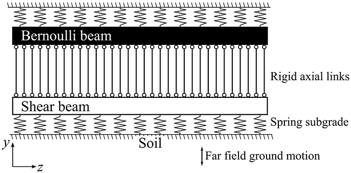
Figure 1. Outline of the developed simplified model.

The equation of motion describing the vibration of the model under the above assumptions can be described as follows (Yu et al., 2016b):

$\begin{array}{cc}\begin{array}{l}EI\frac{{\partial }^{4}u(z,t)}{\partial z^4}-AG\frac{{\partial }^{2}u(z,t)}{\partial z^2}+\rho \frac{{\partial }^{2}u(z,t)}{\partial t^2}+\\ ku(z,t)=-\rho \frac{{\partial }^2{u}_g(z,t)}{\partial t^2}\end{array}& (1)\end{array}$

where: z is the ordinate along the tunnel length, t is time, u is the vertical deflection of the tunnel, EI is the flexural stiffness of the Bernoulli beam, AG is the shear stiffness of the shear beam, k is the Winkler subgrade reaction modulus, ρ is the unitary mass of the tunnel per length, and u_g denotes the far–field uniform vertical ground motion under the foundation.

Equation (1) can be solved through modal analysis. Firstly, its free vibration is governed by the following differential equations:

$\begin{array}{cc}\begin{array}{l}\frac{d^{2}q(t)}{d{t}^2}+\left[{\psi }^2+\frac{k}{\rho }\right]q(t)=0\end{array}& (2)\end{array}$

$\begin{array}{cc}\begin{array}{l}\frac{d^4\varphi (x)}{d{x}^4}-{\alpha }^2\frac{d^2\varphi (x)}{d{x}^2}-{\psi }^2{\tau }^2\varphi (\text{x})=0\end{array}& (3)\end{array}$

where: q determines the temporal nature of the response, φ is the mode shape and ψ [1/s] is the coupling parameter between Equations (2) and (3) that will define the system response; and take a set of discrete infinite values, each one related to a different mode shape. Furthermore, the variable z has been normalized by the tunnel length H (x = z/H) in Equation (3), introducing the following parameters:

$\begin{array}{cc}\begin{array}{l}\alpha =\sqrt{\frac{AG{H}^2}{EI}};\tau =\sqrt{\frac{\rho H^4}{EI}}\end{array}& (4)\end{array}$

where: α is the non-dimensional ratio of shear to flexural stiffness, effectively controlling the role of coupled shear deformation among the supporting springs (Pasternak, 1954; Miranda and Taghavi, 2005), and τ is the tunnel mass parameter normalized by length and flexural stiffness, allowing for definition of a non-dimensional frequency parameter, as ωτ.

From Equation (2) the modal, non-dimensional, circular vibration frequency of the i-th mode is:

$\begin{array}{cc}\begin{array}{l}{\omega }_i\tau =\sqrt{{{\psi }_i}^2{\tau }^2+{k_b}^2}\end{array}& (5)\end{array}$

where k_b is the non-dimensional ratio between subgrade and flexural stiffness defined below,

$\begin{array}{cc}\begin{array}{l}{k}_b=\sqrt{\frac{k{H}^4}{EI}}\end{array}& (6)\end{array}$

The general solution of Equation (3) is given by the following expression:

$\begin{array}{cc}\begin{array}{l}{\varphi }_i(x)=A_{1}sin({\gamma }_{i}x)+A_{2}cos({\gamma }_{i}x)+A_{3}sinh({\beta }_{i}x)+A_{4}cosh({\beta }_{i}x)\end{array}& (7)\end{array}$

where: A₁, A₂, A₃, A₄ are coefficients that depend on the end boundary conditions. The variables γ_i and β_i, which describe the i-th mode shape, are related to model parameters as follows:

$\begin{array}{cc}\begin{array}{l}{{\gamma }_i}^2+{\alpha }^2={{\beta }_i}^2\end{array}& (8)\end{array}$

$\begin{array}{cc}\begin{array}{l}{{\gamma }_i}^4+{{\gamma }_i}^2{\alpha }^2={{\psi }_i}^2{\tau }^2\end{array}& (9)\end{array}$

Consequently, if γ_i and β_i are found, they will define the non-dimensional product ψ_iτ according to Equation (9). With this in hand, it is possible to use Equation (5) to calculate the normalized, non-dimensional, modal circular vibration frequencies. Furthermore, if modal vibration periods are scaled by the first fundamental period, T₁, the following is obtained:

$\begin{array}{cc}\begin{array}{l}\frac{{{\gamma }_i}^4+{{\gamma }_i}^2{\alpha }^2+{k_b}^2}{{{\gamma }_1}^4+{{\gamma }_1}^2{\alpha }^2+{k_b}^2}={\left(\frac{T_1}{T_i}\right)}^2\end{array}& (10)\end{array}$

The above equations fully define the simplified model. Its response to ground motion can be obtained by setting these four parameters: α, k_b, T₁ and the fraction of critical damping for each mode ξ_i.

Fixed–fixed end boundary conditions at the ends are considered, being representative of a tunnel spanning two close-by underground stations. Under such fixed supports at both beam extremities, the following boundary conditions apply for each mode:

$\begin{array}{cc}\begin{array}{l}{{\varphi }_i(x)|}_{x=0}=0_{}{;}_{}{{{\varphi }_i}^{\prime }(x)|}_{x=0}=0_{}{;}_{}{{\varphi }_i(x)|}_{x=1}=0_{}^{}{;}_{}{{{\varphi }_i}^{\prime }(x)|}_{x=1}=0\end{array}& (11)\end{array}$

Applying the above boundary conditions to Equation (7) defines the following system of equations in matrix form:

$\begin{array}{cc}\begin{array}{l}\left[\begin{array}{cccc}0& 1& 0& 1\\ {\gamma }_i& 0& {\beta }_i& 0\\ sin({\gamma }_i)& cos({\gamma }_i)& sinh({\beta }_i)& cosh({\beta }_i)\\ {\gamma }_{i}cos({\gamma }_i)& -{\gamma }_{i}sin({\gamma }_i)& {\beta }_{i}cosh({\beta }_i)& {\beta }_{i}sinh({\beta }_i)\\ \end{array}\right]\left[\begin{array}{c}{A}_1\\ A_2\\ A_3\\ A_4\\ \end{array}\right]=\left[\begin{array}{c}0\\ 0\\ 0\\ 0\\ \end{array}\right]\end{array}& (12)\end{array}$

In order to avoid a null solution to the above system, the determinant in Equation (12) must be zero, leading to the following modal characteristic equation:

$\begin{array}{cc}\begin{array}{l}{\left[{{\gamma }_i}^2-{{\beta }_i}^2\right]}^{}sinh({\beta }_i)sin({\gamma }_i)+2{\gamma }_i{\beta }_i\left[cos({\gamma }_i)cosh({\beta }_i)-1\right]=0\end{array}& (13)\end{array}$

The roots of Equation (13) define the β_i and γ_i parameters needed for evaluating the period ratios in Equation (10), and the following mode shapes:

$\begin{array}{cc}\begin{array}{l}{\varphi }_i(x)={\eta }_{i}sin({\gamma }_{i}x)-cos({\gamma }_{i}x)-\frac{{\gamma }_i}{{\beta }_i}{\eta }_{i}sinh({\beta }_{i}x)+cosh({\beta }_{i}x)\end{array}& (14)\end{array}$

where η_i is:

$\begin{array}{cc}\begin{array}{l}{\eta }_i=\frac{cos({\gamma }_i)-cosh({\beta }_i)}{sin({\gamma }_i)-\frac{{\gamma }_i}{{\beta }_i}sinh({\beta }_i)}\end{array}& (15)\end{array}$

It must be noted that the mode shapes are independent of the value of the subgrade reaction modulus, k_b, as they only depend on γ_i and β_i. This is valid because a uniform support is used as a simplification.

Response to Ground Motion and Modal Properties Verification

Equation (1) can be solved through modal decomposition, and so the displacement is given by (Paz, 2006):

$\begin{array}{cc}u(x,t)={\displaystyle \sum _{i=1}^{N}U{g}_i{r}_i(t)}& (16)\end{array}$

Equation (16) constitutes an exact solution only if an infinite number of modes N is considered, but usually up to 5 modes are sufficient (Miranda and Taghavi, 2005). The values of r_i can be found after solving the following ordinary differential equation:

$\begin{array}{cc}\begin{array}{l}{{\omega }_i}^2{r}_i+2{\xi }_i{\omega }_i{ṙ}_i+{\ddot{r}}_i=-U{g}_i(t)\end{array}& (17)\end{array}$

where Ug_i is the equivalent ground motion for each mode:

$\begin{array}{cc}\begin{array}{l}U{g}_i=\frac{{\displaystyle \underset{0}{\overset{1}{\int }}}{u}_g(x,t){\varphi }_i(x)dx}{{\displaystyle \underset{0}{\overset{1}{\int }}}{{\varphi }_i}^2(x)dx}\end{array}& (18)\end{array}$

However, evaluation of Equation (18) requires knowledge of the ground motion field at all times and positions under the Winkler base. This information cannot be expected to be available under normal circumstances, as it would require deployment of dense sensor networks within the support medium around the tunnel, and would still not provide the exact u_g(x, t) function. Therefore, a more practical and realistic source of excitation data is out-of-site strong motion recording stations. Hence, a more convenient approach is to assume uniform base excitation, in which case Equation (17) becomes:

$\begin{array}{cc}\begin{array}{l}{{\omega }_i}^2{r}_i+2{\xi }_i{\omega }_i{ṙ}_i+{\ddot{r}}_i=-{\Gamma }_i{ü}_g(t)\end{array}& (19)\end{array}$

where parameter Γ_i is given by:

$\begin{array}{cc}\begin{array}{l}{\Gamma }_i=\frac{{\displaystyle \underset{0}{\overset{1}{\int }}}{\varphi }_i(x)dx}{{\displaystyle \underset{0}{\overset{1}{\int }}}{{\varphi }_i}^2(x)dx}\end{array}& (20)\end{array}$

Equation (19) is the same with the one that governs the equation of motion of a Single Degree of Freedom (SDOF) oscillator, except that it is scaled by Γ_i. For the stated model hypotheses, closed form expressions for this parameter are given in Equation (A.1) in Appendix A. In this study, the algorithm developed by Nigam and Jennings (1969) is employed to solve Equation (19) for each mode. Total acceleration is found by taking the second derivative of Equation (16), considering Equation (20) and adding the base ground motion:

$\begin{array}{cc}\begin{array}{c}{ü}_T(x,t)={\displaystyle \sum _{i=1}^N{\Gamma }_i{\varphi }_i(x){\ddot{r}}_i(t)+{ü}_g(t)}\end{array}& (21)\end{array}$

Verification of Modal Parameters

The developed simplified model is verified against the results of a dense finite element (FE) model, which is used as a benchmark. Its correctness will be assessed in the future against field measurements and laboratory tests. The closed–form expressions proposed for both modal period ratios and mode shapes considering the fixed-fixed boundary conditions are used for the comparison.

The FE model is implemented in SAP 2000 (Wilson, 2002). Two beams, comprising 1,000 beam elements each (with a unitary length) are placed next to each other (separated by an unitary distance) and they are subjected to equal vertical displacements. For one of the two beams, the rotation is also constrained (set to zero), while its flexural stiffness is adjusted to represent the shear stiffness associated with the α value being considered. The flexural stiffness of the other beam is set to a unitary value, while its nodes are coupled with springs and unitary (translational) masses. The stiffness of the Winkler springs is adjusted to represent the k_b values.

For buildings, values of α range between 0 and 30 (Alimoradi et al., 2006). As tunnels usually have large length-to-diameter ratios, they are usually idealized as thin-walled cylinders (Kouretzis et al., 2006, 2011). It is expected that their deformation patterns resemble more what is observed in flexural (Bernoulli) beams, rather than shear beams. Consequently, as a first approximation, values between 0 and 20 were considered in this study. Previous research regarding the dynamic behavior of beams on Pasternak foundations considered values up to α = 3 (Valsangkar and Pradhanang, 1988; Filipich and Rosales, 2002).

The parameter k_b takes values between 4 × 10⁻³ H² and 3 × 10⁻² H². The derivation of these values is presented in Appendix B and was achieved by considering the tunnel design recommendations of the Japanese Railway Research Institute, which are based on data inferred from plate tests (Zhang et al., 2014), while adopting a tunnel cross-section similar to the one of the T3 Santiago de Chile Metro Line, which is idealized as a hollow circle of 10 m outer diameter and 0.5 m wall thickness, and concrete modulus of elasticity of 30 GPa. Furthermore, tunnel lengths (H) between 100 and 250 m were considered, which constitute a reasonable spacing between successive metro stations in dense urban areas.

The above values result in k_b limit values of 40 and 1,000. Beyond this upper value, tunnel flexibility is so large that its displacement follows the ground motion, rendering pseudo-static analysis valid (Valsangkar and Pradhanang, 1988)—less interesting in the context of this paper. Hence, based on the above, the following cases are considered: α = 0 and k_b = 5; α = 0 and k_b = 25; α = 7 and k_b = 1; α = 7 and k_b = 1,000; α = 20 and k_b = 10; α = 20 and k_b = 100, representing extreme values. As shown in Figure 2, for all cases examined the comparison proves the correctness of analytical solution, with overall differences between the closed-form solution for period ratios, mode shapes and the benchmark numerical simulations being < 0.1%.

FIGURE 2

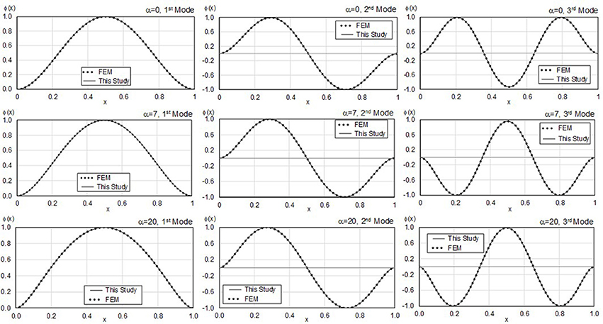
Figure 2. Verification of the simplified model against a dense FE model, assuming fixed ends.

System Identification Algorithm and Results

The simplified model, defined by four parameters, can be used to undertake system identification under the assumption that sensor networks are available to measure actual tunnel response. Setting proper values for parameters describing the model can be done by involving system identification procedures on both frequency (McVerry, 1980) and time domain (Beck and Jennings, 1980) following the outline described in Figure 3.

FIGURE 3

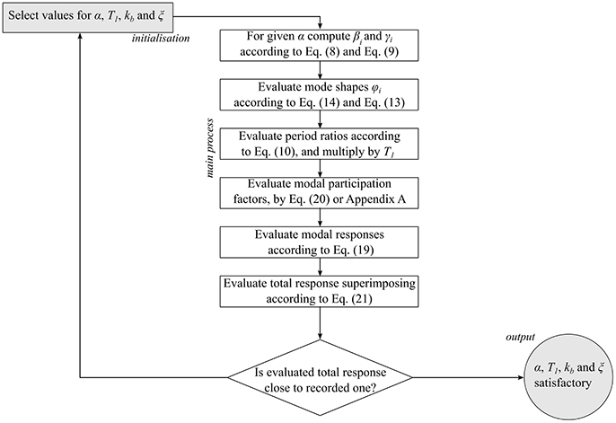
Figure 3. Outline of the System Identification procedure.

The procedure starts by defining an initial set of parameters, which is iteratively updated until the difference between modeled and measured response at the desired locations becomes less than a threshold. In principle, gradient dependent methods (Arora, 2015) could be employed. However, they are prone to yield local instead of global optimal values. An alternative is to use heuristic methods (Bozorg-Haddad et al., 2017), which mimic biological and physical phenomena to systematically search a dominion of plausible values, allowing for aleatory search beyond regions where local minima are observed. It must be stressed that heuristic algorithms cannot guarantee that an absolute minimum is achieved; consequently, it is common practice that the final results based on multiple runs are critically reviewed. In this paper, the square difference between measured and predicted total acceleration time histories is set as the objective function (OF) to be minimized:

$\begin{array}{cc}\begin{array}{l}OF(\alpha ,k_b,T_1,\xi )={\displaystyle \sum _{j=1}^n}{\left[{ü}_T(\alpha ,k_b,T_1,\xi ,x_j)-{ü}_{T_M}(x_j)\right]}^2\end{array}& (22)\end{array}$

where: n is the number of total acceleration time histories recorded (ü_TM) at locations x_j.

Genetic Algorithms

Among Heuristic methods, Genetic Algorithms (GA) and GA-based procedures have been employed widely to solve problems in geomechanics, including the estimation of lateral load capacity of piles, undrained side resistance of drilled shafts, tunneling-induced ground motion settlements, and soil liquefaction (Gandomi and Alavi, 2012).

GA are programming schemes for searching a domain space involving a process that mimics natural selection of biological species (Affenzeller et al., 2009); firstly, initial values (“first generation”) of parameters are generated randomly. Each full set of parameters (α, k_b, T₁, and ξ) constitutes an individual. Once the first generation is produced, the OF for all individuals is calculated and the best performing become “parents”. These parents are then combined through a process called crossover to define new individuals, called “children”. In this study, crossover is done through roulette selection, in such way that the chances of being selected for crossover are proportional to the inverse value of the OF, i.e., the lower the OF it is, the higher the possibility of being combined with another high-valued individual.

Crossover is made through a weighted average of parameters that comprise each parent. Weights are defined according to the value of OF for each one of them. Therefore, parameters in children will resemble mostly the parent with the lowest OF value. Also, the algorithm introduces aleatory modifications randomly in children parameters, following a prescribed probability of occurrence. This process is called “mutation”. Finally, all samples are ranked. The best suited individuals are included in the next generation, while the worst performing ones are discarded. The process continues until no meaningful improvement in minimizing the OF is found. In this study, the algorithm is implemented using Matlab Optimization Toolbox function GA (The Mathworks, 2016), with the following parameters: population size of 50 individuals, 400 maximum allowable generations, a stop criterion if changes in the OF are < 10⁻⁶ and 5% chance of mutation.

Investigated Cases

Ten discrete samples were selected from a wide range of possible values for each one of the four parameters describing the model. A range of indicative values is considered for each variable: α ranges from 1 to 19; k_b between 1 and 400; T₁ between 0.3 and 1.2 s (Wang et al., 2015); and ξ (which was considered uniform for all modes) between 0.5 and 5%. Then, 10 random combinations of these parameters were created, leading to the test cases outlined in Table 1.

TABLE 1

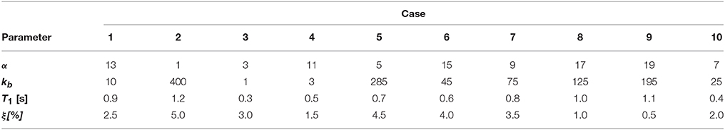
Table 1. Test cases.

The vertical component of two ground motions were selected to excite the model at its base: the Hulverstone Drive Pumping Station (HDPS) record, obtained within the city of Christchurch, during its 2011 M_w 6.2 earthquake, and the CHY080 record obtained during the 1999 M_w 7.6 Chi-Chi Taiwan earthquake mainshock. Both records are characterized by high peak ground acceleration (PGA) values in the vertical direction, i.e., 10.5 m/s² for HDPS and 7.50 m/s² for CHY80. The different acceleration spectral response of each motion is presented in Figure 4 (Pacific Earthquake Engineering Research Center, 2018).

FIGURE 4

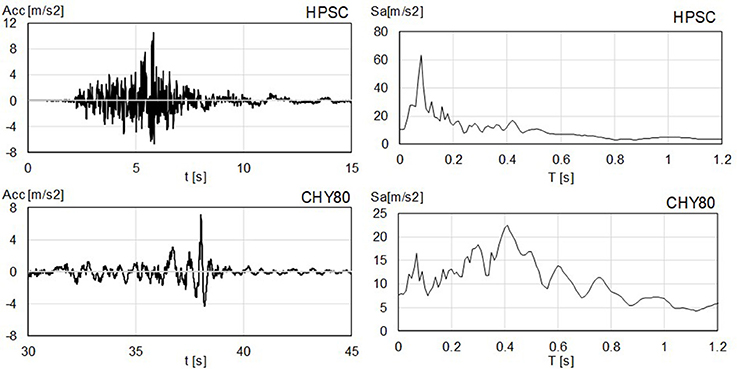
Figure 4. Ground motions considered in this study. Time histories on left, acceleration response spectra (ξ = 2%) on right.

The model response was recorded at 9 locations, considering 3 configurations: uniformly spaced along the full length; clustered in the middle between x = 0.3 and x = 0.7 considering spacing half the one employed in the uniform case; and deployed just in the first half (x ≤ 0.5) again with half the spacing of the uniform layout. Additionally, the records of all sensors were compromised by adding independent white Gaussian noise with a variance equal to the one observed for the ground motion. Finally, a reduced network of only 5 sensors, deployed at x = 0.2, 0.4, 0.5, 0.6, 0.8 was assessed fora subset made by the best performing tests cases, i.e., 1, 6 and 7 (see Table 1 for naming convention).

Results

As summarized in Table 2, for values of T₁ < 0.5 s the algorithm is unable to recover a useful solution. Beyond this limit, the algorithm successfully recovers model parameters, with divergences < 5% in more than 75% of all runs as long the fundamental period is < 1 s and in more than 50% for values beyond that threshold. Among successfully obtained parameters, differences between estimates and target values are < 1% in more than 90% of successful runs, and in all cases < 2%. Indicative target against estimated responses are shown in Figure 5.

TABLE 2

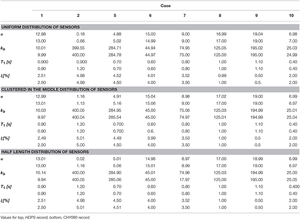
Table 2. Best recovered parameters.

FIGURE 5

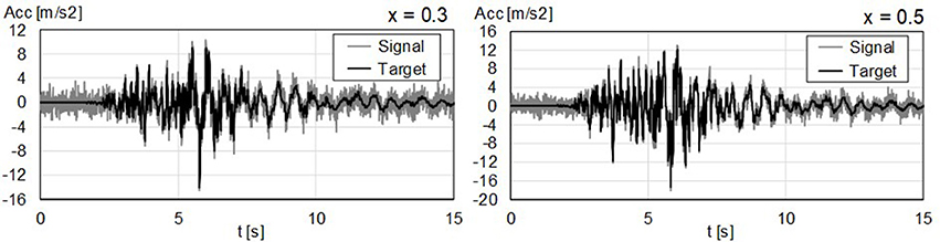
Figure 5. Target (in black) and simulated model response. Case 6, HPSC ground motion.

Case 2 is particularly interesting because the α value is not well estimated, ranging between 0 and 1.3. This is because for values of α below 3.0 the influence of this parameter in the acceleration response is small: this was observed by the small variations in the mode shapes and period ratios for α < 3 as shown in Figure 6. In other words, for this range of values, considering the Bernoulli Beam on a spring base is a reasonable approximation, as changes in a value for this range produce slight changes on acceleration response. Beyond 3.0, the effects of α become more pronounced, noticeably influencing acceleration response and therefore, allowing the algorithm to capture them more accurately.

FIGURE 6

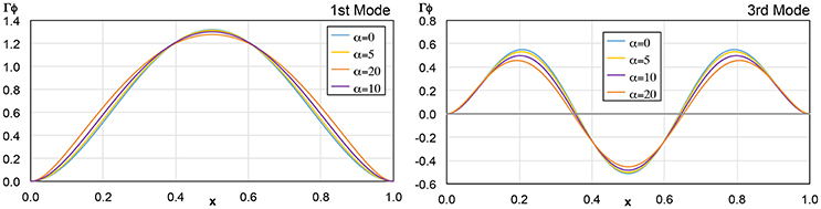
Figure 6. Effect of α in mode shapes. First and third modes.

Effects of changes in sensor arrangement on finally predicted results are not significant. Relevant predicted parameters can be recovered from any of the assessed sensor layouts. Also, results for the reduced array of just 5 sensors were proven satisfactory (Table 3). Furthermore, recovered parameters match closely the target values, showing results that are comparable to what was observed for the denser 10 sensor arrangement.

TABLE 3

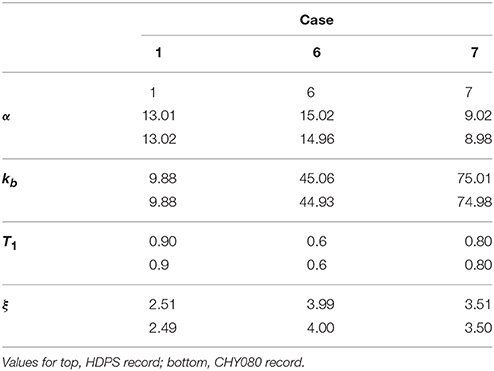
Table 3. Best recovered parameters, arrangement of 5 sensors.

Conclusions

The use of a simplified model for system identification of tunnels considering earthquake–induced ground motion is presented in this paper. The model includes coupled flexural and shear beams, supported by Winkler-type springs, in such way that they are subjected to the same vertical accelerations. The proposed model effectively extends a previous model, which was developed for buildings. Closed form solutions for modal assessment of response were obtained in terms of trigonometric and hyperbolic functions. These solutions were verified against the results of a dense FE model, used as a benchmark.

It was shown that the proposed simplified model can be properly defined by 4 parameters only; the first mode period T₁; the ratio α of shear to flexural stiffness; the ratio k_b between subgrade stiffness and flexural beam stiffness; and the overall damping ratio ξ for each mode.

Using a simple genetic algorithm and the proposed simplified model, it was shown that a system identification can be performed for variable conditions. The model was tested for two different earthquakes of varied frequency content, and the influence of sensor distribution along the tunnel length was parametrically investigated. The output of tests was intentionally compromised by adding white Gaussian noise with a variance equal to the one observed in the ground motion. It was observed that for α values >3.0 (i.e., when the effect of the shear beam is of significance), model parameters can be successfully recovered. Hence, for such conditions, the proposed approach can be used to recover important dynamic properties of the tunnel (e.g., T₁ or α), but also soil-structure interaction by tracking changes of k_b following earthquakes. For values < 3, the Bernoulli beam with a Winkler Base is a valid representation, observing differences with a model including a Pasternak foundation to be marginal.

The different sensor distributions and the reduced number of sensors did not lead to significant differences in the final results. This initially shows that sensor position is not the dominating parameter for the case of 5 sensors along a tunnel length fixed at both ends, and the uniform ground conditions and other assumptions made in the paper. Further tests should be conducted on real data and sensors to study the influence of other aspects such as sensor noise.

List of Variables

A: coefficients of the general modal solution.

AG: shear stiffness. [N]

EI: flexural Stiffness. [Nm²]

H: tunnel length. [m]

k: Winkler grade reaction modulus. [N/m/m]

k_b: non-dimensional, normalized Winkler reaction coefficient by flexural stiffness.

i: mode index.

OF: Objective Function.

q(t): time variation of modal ordinate during free vibration.

r: time variation of modal ordinates when subjected to ground motion.

T: mode vibration period.

u: vertical deflection of the tunnel. [m]

u_g: displacement at the base of the Bernoulli beam. [m]

ü_T: total tunnel acceleration.

ü_TM: measured tunnel acceleration.

U_g: generalized displacement at the base. [m]

x: normalized length ordinate by tunnel length.

x_j: normalized location of j-th sensor.

z: ordinate along tunnel length. [m]

α: non-dimensional ratio between shear and flexural stiffness.

β_i: parameter of the i-th mode shape.

γ_i: parameter of the i-th mode shape.

Γ_i: i-th mode Participation Factor.

η_i: parameter of the i-th mode shape.

φ_i(x), i-th mode shape.

ψ: coupling parameter between Equation (2) and Equation (3).

ξ_i: damping coefficient to the critical (for mode i).

ρ: mass per unit length. [kg/m]

τ: normalized mass parameter normalized by flexural stiffness. [1/s]

ω: circular vibration frequency of mode i. [1/s].

Author Contributions

AA-R: Development of the model and implementation of the Test Algorithm; RF: Development of the model and revision of paper draft; NN: Development of tests cases, definition of the Test Algorithm; JK and GK: Definition of Range of test parameters, Review of Paper and Validation of the Model; IA: Definition of the System Identification Algorithm, Final review of the document.

Conflict of Interest Statement

The authors declare that the research was conducted in the absence of any commercial or financial relationships that could be construed as a potential conflict of interest.

Acknowledgments

This work was sponsored by a Newton Fund Initiative, supported jointly by the Engineering and Physical Sciences Research Council of the UK and the National Commission for Scientific and Technological Research of Chile, grant EP/N03435X/1. Strong motion records employed in this work were obtained from the PEER NGA 2 database, hosted by the Pacific Earthquake Engineering Research Center.

References

Affenzeller, M., Winkler, S., Wagner, S., and Beham, A. (2009). Genetic Algorithms and Genetic Programming. Boca Raton, FL: CRC Press.

Google Scholar

Alimoradi, A., Miranda, E., Taghavi, S., and Naeim, F. (2006). Evolutionary modal identification utilizing coupled shear-flexural response-implications for multistory buildings. Struct. Des. Tall Spec. Build. 15, 51–65. doi: 10.1002/tal.343

CrossRef Full Text | Google Scholar

Anastasopoulos, I., Gerolymos, N., Drosos, V., Kourkoulis, R., Georgarakos, T., and Gazetas, G. (2007). Nonlinear response of deep immersed tunnel to strong seismic shaking. J.Geotech. Geoenviviron Eng. 133, 1067–1090. doi: 10.1061/(ASCE)1090-0241(2007)133:9(1067)

CrossRef Full Text | Google Scholar

Arora, R. K. (2015). Optimization: Algorithms and Applications. London: Chapman and Hall/CRC.

Google Scholar

Beck, J. L., and Jennings, P. C. (1980). Structural Identification using linear models and earthquake records. Earthquake Eng. Struct. Dyn. 8, 145–160. doi: 10.1002/eqe.4290080205

CrossRef Full Text | Google Scholar

Bennett, P. J., Kobayashi, Y., Soga, K., and Wright, P. (2010). Wireless sensor network for monitoring transport tunnels. ICE Geotech. Eng. 163, 147–156. doi: 10.1680/geng.2010.163.3.147

CrossRef Full Text | Google Scholar

Bhalla, S., Yang, Y. W., Zhao, J., and Soh, C. K. (2005). Structural health monitoring of underground facilities – technological issues and challenges. Tunnel. Underground Space Technol. 20, 487–500. doi: 10.1016/j.tust.2005.03.003

CrossRef Full Text | Google Scholar

Bozorg-Haddad, O., Solgi, M., and Loaiciga, H. A. (2017). Meta-heuristic and Evolutionary Algorithms for Engineering Optimization. Hooboken, NJ: Wiley-Blackwell.

Google Scholar

Celebi, M. (2007). “On the variation of fundamental frequency (period) on an undamaged building – a Continuing Discussion,” in International Conference on Experimental Vibration Analysis for Civil Engineering Structures. Porto.

Google Scholar

Dikmen, S. U. (2016). Response of marmaray submerged tunnel during the 2014 Northern Aegean Earthquake (Mw = 6.9). Soil Dyn. Earthquake Eng. 90, 15–31. doi: 10.1016/j.soildyn.2016.08.006

CrossRef Full Text | Google Scholar

Dolce, M., Nicoletti, M., De-Sortis, A., Marchesini, S., Spiuna, D., and Talanas, F. (2017). Osservatorio sismico delle strutture: the italian structural seismic monitoring network. Bull. Earthquake Eng. 15, 621–641. doi: 10.1007/s10518-015-9738-x

CrossRef Full Text | Google Scholar

Filipich, C., and Rosales, M. B. (2002). A further study about the behaviour of foundation piles and beams in a Winkler-Pasternak Soil. Int. J. Mech. Sci. 44, 21–36. doi: 10.1016/S0020-7403(01)00087-X

CrossRef Full Text | Google Scholar

Fraser, M., Elgamal, A., He, X., and Conte, J. P. (2010). Sensor network for structural health monitoring of a highway bridge. J. Comput. Civil Eng. ASCE 24, 11–24. doi: 10.1061/(ASCE)CP.1943-5487.0000005

CrossRef Full Text | Google Scholar

Gandomi, A., and Alavi, A. (2012). A new multi-gene genetic programming approach to non-linear system modeling. Part II: geotechnical and earthquake engineering problems. Neural comput. Appl. 21, 189–201. doi: 10.1007/s00521-011-0735-y

CrossRef Full Text | Google Scholar

Girija-Vallabhan, C. V., and Das, Y. C. (1991). A refined model for beams on elastic foundations. Int J. Solids Struct. 27, 629–637. doi: 10.1016/0020-7683(91)90217-4

CrossRef Full Text | Google Scholar

Hatzigeorgiou, G. D., and Beskos, D. E. (2010). Soil-Structure interaction effects on seismic inelastic analysis of 3-D Tunnels. Soil Dyn. Earthquake Eng. 30, 851–861. doi: 10.1016/j.soildyn.2010.03.010

CrossRef Full Text | Google Scholar

Karadeniz, H. (2001). Earthquake analysis of buried structures and pipelines based on Rayleigh wave propagation. Int. J. offshore Polar Eng. 11, 133–140. Available online at: http://legacy.isope.org/publications/journals/journalJune01.htm

Google Scholar

Kouretzis, G. P., Bouckovalas, G. D., and Gantes, C. J. (2006). 3-D shell analysis of cylindrical underground structures under seismic shear (S) wave action. Soil Dyn. Earthquake Eng. 26, 909–921. doi: 10.1016/j.soildyn.2006.02.002

CrossRef Full Text | Google Scholar

Kouretzis, G. P., Bouckvalas, G. D., and Karamitros, D. K. (2011). Seismic verification of long cylindrical Underground structures considering Rayleigh wave effects. Tunel. Underground Space Technol. 26, 789–794. doi: 10.1016/j.tust.2011.05.001

CrossRef Full Text | Google Scholar

Li, H., Ren, L., Jia, Z., Yi, T., and Li, D. (2016). State-of-the-art in structural health monitoring of large and complex civil infrastructures. J. Civil Struct. Health Monit. 6, 3–16. doi: 10.1007/s13349-015-0108-9

CrossRef Full Text | Google Scholar

Loh, C., and Chen, J. (2017). Tracking modal parameters from building seismic response data using recursive subspace identification algorithm. Earthquake Eng. Struct. Dyn. 46, 20163–22183. doi: 10.1002/eqe.2900

CrossRef Full Text | Google Scholar

McVerry, G. H. (1980). Structural identification in the frequency domain from earthquake records. Earthquake Eng. Struct. Dyn. 8, 161–180. doi: 10.1002/eqe.4290080206

CrossRef Full Text | Google Scholar

Mikael, A., Gueguen, P., Bard, P., Roux, P., and Langlais, M. (2013). The analysis of long-term frequency and damping wandering in buildings using the random decrement technique. Bull. Seismol. Soc. Am. 113, 236–246. doi: 10.1785/0120120048

CrossRef Full Text | Google Scholar

Miranda, E. (1999). Approximate seismic lateral deformation demands in multistory buildings. J. Struct. Eng. 125, 417–425. doi: 10.1061/(ASCE)0733-9445(1999)125:4(417)

CrossRef Full Text | Google Scholar

Miranda, E., and Taghavi, S. (2005). Approximate floor acceleration demands in multi-story buildings I: formulation. J. Struct. Eng. ASCE 131, 203–211. doi: 10.1061/(ASCE)0733-9445(2005)131:2(203)

CrossRef Full Text | Google Scholar

Nigam, N. C., and Jennings, P. C. (1969). Calculation of response spectra from strong-motion earthquake records. Bull. Seismic. Soc. Am. 59, 909–922.

Google Scholar

Nogami, T., and Lam, Y. C. (1987). Two-parameter layer model for analysis of slab on elastic foundation. J. Eng. Mech ASCE 113, 1279–1291. doi: 10.1061/(ASCE)0733-9399(1987)113:9(1279)

CrossRef Full Text | Google Scholar

Ogie, R. I., Perez, P., and Dignum, V. (2017). Smart infrastructure: an emerging frontier for multidisciplinary research. Smart Infrastruct. Construct. ICE 170, 8–16. doi: 10.1680/jsmic.16.00002

CrossRef Full Text | Google Scholar

Oh, J., and Moon, T. (2018). Seismic design of a single bored tunnel: longitudinal deformations and seismic joints. Rock Mech. Rock Eng. 51, 891–910. doi: 10.1007/s00603-018-1434-0.

CrossRef Full Text | Google Scholar

Osawa, Y. (1965). Response analysis of tall buildings to strong earthquake motions. Part 1: linear response of core-wall buildings. Bull. Earthquake Res. Inst. 43, 803–817.

Pacific Earthquake Engineering Research Center, P. E. E. R. (2018). NGA-West 2 Peer Ground Motion Database. Available online at: https://ngawest2.berkeley.edu/site (Accessed April 18, 2018).

Pasternak, P. (1954). On a New Method of Analysis of an Elastic Foundation by Means of Two Foundation Constants. Moscow:Gosudarstvenrwe Izdatelslvo Literaturi po Stroitclstvu i Arkhitekture (In Russian).

Paz, M. (2006). Structural Dynamics: Theory and Computation. 5th Edn Berlin: Springer.

Saaed Alqado, T. E., Nikolakopoulos, G., and Jonasson, J. (2015). Comfort level identification for irregular multi-storey buildings. Automat. Const. 50, 40–49. doi: 10.1016/j.autcon.2014.10.009

CrossRef Full Text | Google Scholar

Sanchez-Merino, A., Fernandez-Saez, J., and Navarro, C. (2009). Simplified longitudinal response of tunnel linings subjected to surface waves. Soil Dyn. Earthquake Eng. 29, 579–582. doi: 10.1016/j.soildyn.2008.06.003

CrossRef Full Text | Google Scholar

St. John, C., and Zarah, T. (1987). Aseismic design of underground structures. Tunnel. Underground Space Technol. 2, 165–197. doi: 10.1016/0886-7798(87)90011-3

CrossRef Full Text | Google Scholar

The Mathworks I. N. C. (2016). Natick, MA: MATLAB V.2016b.

Tondini, N., Bursi, O., Bonelli, A., and Fassin, M. (2015). Capabilities of the Fiber Bragg Sensor System to monitor the inelastic response of concrete sections in new tunnel linings subjected to earthquake loading. Comput. Aid. Civil Infrastruct. Eng. 30, 636–656. doi: 10.1111/mice.12106

CrossRef Full Text | Google Scholar

Towhata, I. (2008). Geotechnical Earthquake Engineering. Berlin, Germany: Springer Science & Business Media.

Google Scholar

Valsangkar, A. J., and Pradhanang, R. (1988). Vibrations of beam-columns on two-parameter elastic Foundations. Earthquake Eng. Struct. Dyn. 16, 217–225. doi: 10.1002/eqe.4290160205

CrossRef Full Text | Google Scholar

Wang, B., Zhang, Z., He, C., and Zheng, H. (2017). Implementation of a long-term monitoring approach for the operational safety of highway tunnel structures in a severely seismic area of China. Struct. Control Health Monitor. 24, 1–18. doi: 10.1002/stc.1993

CrossRef Full Text | Google Scholar

Wang, Z.Z., Jiang, Y.-J., Zhu, C.A., and Sun, T.C. (2015). Shaking table tests of tunnel linings in progressive states of damage. Tunnel. Underground Space Technol. 50, 109–117. doi: 10.1016/j.tust.2015.07.004

CrossRef Full Text | Google Scholar

Wilson, E. (2002). Sap2000 Integrated Software for Structural Analysis and Design, Analysis Reference Manual. Berkeley, CA: Computers and Structures Inc.

Winkler, E. (1867). Die Lehre von der Elasticitaet und Festigkeit. Theil, 2. Prague: H. Dominicus (in German).

Wu, D., and Gao, B. (2013). Dynamic analysis of tunnel entrance under the effect of Rayleigh wave. Electron. J. Geothech. Eng. 18, 4231–4246.

Google Scholar

Younan, A., Veletsos, A., and Bandyopadhyay, K. (1997). Dynamic Response of Flexible Retaining Walls. Report BNL 52519, Department of Advanced Technology, Brookhaven National Laboratory, Upton, NY.

Google Scholar

Yu, H., Cai, C., Guan, X., and Yuan, Y. (2016b). Analytical solution for long lined tunnels subjected to travelling loads. Tunnel. Underground Space Technol. 58, 209–215. doi: 10.1016/j.tust.2016.05.008

CrossRef Full Text | Google Scholar

Yu, H., Chen, J., Bobet, A., and Yuan, Y. (2016a). Damage observation and assessment of the Longxi tunnel during the Wenchuan earthquake. Tunnel. Underground Space Technol. 54, 102–116. doi: 10.1016/j.tust.2016.02.008

CrossRef Full Text | Google Scholar

Yu, H., Yuan, Y., and Bobet, A. (2017). Seismic analysis of long tunnels, a review of simplified and unified methods. Underground Space 2, 73–87. doi: 10.1016/j.undsp.2017.05.003

CrossRef Full Text | Google Scholar

Zhang, D., Huang, H., Phoon, K. K., and Hu, Q. A. (2014). Modified solution of radial subgrade modulus for a circular tunnel in elastic ground. Soils Found. 54, 225–232. doi: 10.1016/j.sandf.2014.02.012

CrossRef Full Text | Google Scholar

Appendices

Appendix A

The solution to Equation (20) is provided below for completeness.

$\begin{array}{l}{\Gamma }_i=\frac{{\Gamma }_{i}NFF}{{\Gamma }_{i}DFF}\\ {\Gamma }_{iNFF}=\frac{{\eta }_i-{\eta }_i\cos ({\gamma }_i)}{{\gamma }_i}+\frac{{\gamma }_i{\eta }_i}{{\beta }_i{}^2}-\frac{\sin ({\gamma }_i)}{{\gamma }_i}+\frac{1}{2}\left[\frac{1}{{\beta }_i}-\frac{{\gamma }_i\eta }{{\beta }_i{}^2}\right]e^{{\beta }_i}-\frac{1}{2}\left[\frac{1}{{\beta }_i}+\frac{{\gamma }_i{\eta }_i}{{\beta }_i^2}\right]e^{-{\beta }_i}\\ {\Gamma }_{i}DFF=\frac{1}{4}\left(-\frac{2{\eta }_i}{{\gamma }_i}+\frac{2{\gamma }_i{\eta }_i}{{\beta }_i{}^2}+\frac{2{\eta }_i\cos (2{\gamma }_i)}{{\gamma }_i}-\frac{{\eta }_i{}^2-1}{{\gamma }_i}\sin (2{\gamma }_i)\right)+\frac{1}{4{\beta }_i{}^3}\left(4{\beta }_i{}^3+2{\beta }_i({\beta }_i-{\gamma }_i)({\beta }_i+{\gamma }_i){\eta }_i{}^2\right)\\ +\frac{\left(A_i+B_i+C_i\right)}{8}{e}^{{\beta }_i}+\frac{\left(B_i+C_i-A_i\right)}{8}{e}^{-{\beta }_i}+\frac{\left(D_i+E_i\right)}{8}{e}^{2{\beta }_i}+\frac{\left(D_i-E_i\right)}{8}{e}^{-2{\beta }_i}\\ A_i=-\frac{8({\beta }_i-{\gamma }_i{\eta }_i)(\beta +{\gamma }_i{\eta }_i)\cos ({\gamma }_i)}{{\beta }_i({\beta }_i{}^2+{\gamma }_i{}^2)};B_i=-\frac{8\sin ({\gamma }_i){\gamma }_i(1+{\eta }_i{}^2)}{{\beta }_i{}^2+{\gamma }_i{}^2};\\ C_i=\frac{8\sin ({\gamma }_i){\eta }_i}{{\beta }_i};D_i=\frac{-2{\gamma }_i{\eta }_i}{{\beta }_i{}^2};E_i=\frac{{\beta }_i{}^2+{\gamma }_i{}^2{\eta }_i{}^2}{{\beta }_i{}^3}.& (\mathrm{A.1})\end{array}$

Appendix B

Reference values are based on the cross section of the Santiago Metro L3 line. Its section can be idealized as circular, with 9m internal and 10m external diameter. Consequently, the second moment of inertia is:

$$\begin{array}{ll}I=\frac{\pi }{4}·\left(5^4-{4.5}^4\right)=170m^4& (\mathrm{B.1})\end{array}$$

and the outer, perimeter:

$\begin{array}{ll}P=\pi ·10=31.4m& (\mathrm{B.2})\end{array}$

Zhang et al. (2014), based on specifications by the Japanese Railway Research Institute and Chinese standards, outline design values for plate reaction modulus of tunnels (k_p) between 3 and 150 MPa/m. This would lead to the following thresholds for the base spring coefficient

$\begin{array}{cc}\begin{array}{l}k=k_p{P}_{}^{}\end{array}& (\mathrm{B.3})\end{array}$

$\begin{array}{cc}\begin{array}{l}{k}_{low}=31.4x0.3=100MN/m;\\ k_{high}=31.4x150=4700MN/m\end{array}& (\mathrm{B.4})\end{array}$

If concrete with 28 day cylinder strength of 35 to 50 MPa is assumed as material with Young's modulus of 35 GPa, the threshold values for the k_b parameter can be computed as:

$\begin{array}{l}{k}_{blow}=\sqrt{\frac{4700H^4}{35x1000x170}}=0.028H^2;\\ \begin{array}{l}{k}_{bhigh}=\sqrt{\frac{10H^4}{35x1000x170}}=0.004H^2\end{array}& (\mathrm{B.5})\end{array}$