Deployment and Shape Change of a Tensegrity Structure Using Path-Planning and Feedback Control

1. Introduction

Many deployable structures today, such as retractable roofs (Gantes et al., 1989; Akgün et al., 2011) and spacecraft appendages (Pellegrino, 1995; Liu et al., 2014) deploy along one-degree of freedom. Tensegrity structures are light-weight and deformable structures that are useful in applications such as flat roofs (Csölleová, 2012), floors (Fest et al., 2004; Motro et al., 2006), shells (Skelton et al., 2001), and towers (Schlaich, 2003). These structures are composed of bars in compression surrounded by a network of cables in tension to maintain stability (Pellegrino and Calladine, 1986; Motro, 2011; Snelson, 2012). Since members are closely coupled, they provide opportunities for testing advanced control algorithms for deployment (Sultan and Skelton, 2003). Tensegrity structures require self-stress; otherwise the structure is unstable due to mechanisms (Schenk et al., 2007). In order to control the structure, either struts (Averseng and Dubé, 2012; Amendola et al., 2014) or cables (Sultan, 2014) have been actuated for shape control.

Experimental testing of a near-full-scale multi-module hollow-rope pedestrian bridge, originally proposed by Motro et al. (2006), has established that deployment with continuous cables was feasible (Veuve et al., 2015). In the first deployment stage, it was observed that empirical deployment resulted in large variations in end-node coordinates. In a second stage, control feedback, proposed by Veuve et al. (2016), has enabled subsequent control-commands that join the connector nodes and ensure successful locking of the two halves. Although control cases were reused by Veuve et al. (2017) for faster and effective control during midspan connection, the deployment trajectory was often uneven, thus limiting efforts to further reduce deployment time.

Sultan and Skelton (2003) presented work of a deployment trajectory close to the equilibrium manifold of a small-scale tensegrity tower approximately 40 [cm] tall. Rhode-Barbarigos et al. (2010a) developed a deployment-path space to avoid strut contact of a pentagonal modular tensegrity structure that deploys along several degrees of freedom. An improvement by Bel Hadj Ali et al. (2011) on the fluidity of control involved the use of actuated continuous cables. This reduced the number of actuators required for effective control as had been proposed by Moored and Bart-Smith (2009).

When a trajectory is uncertain, path planning algorithms such as rapidly exploring random trees (RRT) (Kuffner and La Valle, 2000), including a quick-convergence extension called RRT star (RRT*) (Islam et al., 2012), for example, support navigation of a search space around obstacles. This algorithm is applied in robotics such as work by Pharpatara et al. (2017) for aerial vehicles in 3-D space for a near-optimal trajectory. RRT* was applied for path planning (Xu et al., 2014) and for simulation of structural control. No experimental application of the RRT algorithm on a physical tensegrity structure has been found.

The RRT path-planning algorithm simulates movement of the tensegrity structure (Ashwear and Eriksson, 2017). Boundaries of the search space are defined by the location of struts to avoid element contact and the resulting unwanted bending forces. Basic RRT algorithm fills the search space (Kuffner and La Valle, 2000) with a process called EXTEND, from an origin with vertices. In large search spaces, the random search quickly explores the space where the Voronoi regions are tessellations originating from a seed point. The probability of a vertex being selected for the EXTEND process is proportional to the area of the Voronoi region using a greedy algorithm. This tree growth is continued and navigates around boundaries by comparing the position of the new point with the limitations of the model.

Using the methodology of RRT connect (Xu et al., 2014), two search trees are created, one at the current position and one at the target position. The goal is to find the path between two configurations, which is discretized into a sequence of configurations for the collision avoidance. The search space is filled with vertices starting from these two origins until the trees meet and fill the entire search space, a process is called CONNECT. RRT-CONNECT continues to expand the two trees until either a boundary is contacted or configuration of the current step is achieved. At this point, roles of the two trees are swapped to allow both trees to extend into the search space. Path-planning is successful when vertices from the initial and target positions are connected while remaining in the search space.

Shape control of tensegrity structures is a challenge due to factors such as friction effects at nodes. These effects were accommodated using the minimum-time method to optimize simulated structural control (Aldrich and Skelton, 2003). As the scale and degree of movement in a tensegrity structure increases, Rieffel et al. (2009) and Rhode-Barbarigos et al. (2010b) observed that challenges associated with construction of the nodes connecting struts and cables also increased. These challenges often increased the difference between simulated and measured deployment behavior. Deployment of a near-full-scale tensegrity structure without significant end-node position variation has not been possible in the laboratory (Veuve et al., 2016, 2017). It is therefore unlikely that a similar full-scale structure in service would be able to achieve repeatable deployed nodal positions. This provides an opportunity to develop and test algorithms that accommodate such variation.

An adaptive modular tensegrity structure was used to study control commands for small deflections (Domer and Smith, 2005). Hierarchical selection for multi-objective shape control of an adaptable tensegrity structure by Adam and Smith (2008) has employed objectives sequentially to reduce the solution set until one solution remained. Strategies such as multiple-limit criteria decision-making have not yet been studied for deployment control algorithms.

Soft constraints are limits that can be relaxed should the deviation from that limit show overall improvement to performance of the system (Tanrikulu et al., 1997). Hard constraints cannot be relaxed. A combination of hard and soft constraints has been used for multi-modulus blind frequency analysis (Abrar et al., 2005; Akande et al., 2016). In the field of structural engineering Smith and Boulanger (1994) explored the use of soft constraints for structural design decision making.

This paper describes a novel methodology for deployment of a near-full-scale pedestrian bridge. Development of a feedback control method of deployment is proposed to adjust predetermined control commands based on variation between measurements and simulation. Then, a description is presented of a path-planning method involving sequential implementation of the following three stages for deployment: (i) use of a path-planning algorithm, (ii) even deployment of all cables, and (iii) feedback-based midspan connection. Finally, a formulation of a stress control method provides the primary optimization criterion for shape control and movement. For self-stress, a multi-criteria strategy is proposed to ensure desired shape and axial forces in elements. Two algorithms, soft-constraint and hard-constraint, are evaluated by simulating self-stress in the tensegrity structure after deployment.

2. Experimental Study

2.1. Tensegrity Structure

The topology shown in Figure 1 is called a “hollow-rope” and it was proposed by Motro et al. (2006) for a pedestrian footbridge. The analytical model of the structure does not include the deck. At full-scale, the center opening of the 16 m-long bridge would be large enough for pedestrian traffic. The structure used for the experiment takes advantage of a closely-coupled multi-element configuration that deploys along several degrees of freedom.

FIGURE 1

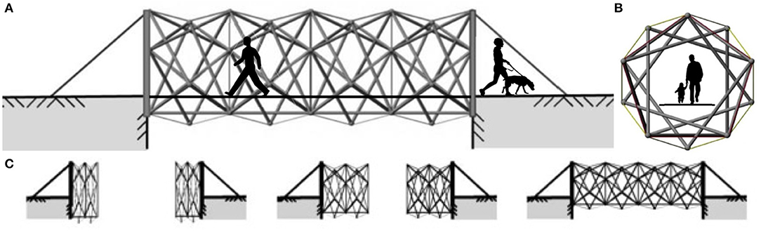
Figure 1. Side (A) and front (B) views of tensegrity footbridge. Deployment of the structure (C) is shown in three stages.

Figure 2 shows a 1/4-scale tensegrity structure from above in a folded state before deployment (a) and after deployment and connection at midspan (b). Numbers correspond to the continuous (active) cables that move the structure. Number of active cables is determined by the topology of the tensegrity structure, which is a pentagonal “hollow rope” (Motro et al., 2006) and therefore, five active continuous cables per half of the structure were installed. Springs, electromagnets, and continuous cables are labeled. The structure is 4 m long and each bridge half weighs 100 kg.

FIGURE 2

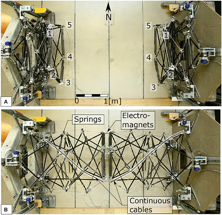
Figure 2. Top view of the tensegrity structure before (A) and after (B) deployment and connection at midspan using electromagnets. Actuation is facilitated by continuous cables and springs on each half of the structure [Credit: IMAC, EPFL].

Self-weight of the structure causes a deflection such that it is necessary to connect node pairs sequentially. A discontinuous cable is a segment of cable that mechanically joins two nodes. A continuous cable has at least one intermediate sliding contact point along its length between its terminal nodes. All continuous cables start from motors at the support nodes and end at the midspan nodes. Actuation of the structure originates from motors through winding and unwinding of cables onto drums at the supports. The structure is kinematically indeterminate and stable under self-stress.

Each pentagonal ring module has fifteen springs, twenty discontinuous cables, thirty struts, and five continuous active cables. Struts are 1.35 m long, 28 mm in diameter, and 1.5 m thick S355 steel tubes. Cables are stainless steel 3 mm in diameter and braided. Steel springs are less stiff at the supports (2.0 kN/m) than in the rest of the structure (2.9 kN/m).

Figure 3 shows five degrees of movement: overall lengthening, helical rotation, constriction, translational movement, and vertical movement. Length change of the structure is generated by the extension and retraction of continuous cables running through the structure. Continuous cables are connected to nodes that form an arc that avoid acute angles formed at joints. This causes the structure to rotate and the diameter to reduce throughout the deployment process. To accommodate this change in diameter, the supports of the structure are placed on rails (Veuve et al., 2015).

FIGURE 3

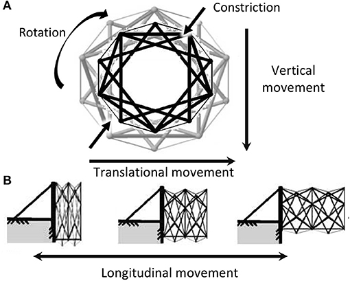
Figure 3. Front (A) and side (B) views of translations, vertical, longitudinal movements of the deployable tensegrity structure. The sketch does not show the effect of gravity and translational movement of the section due to continuous cable positions.

Deflection at midspan is due to self-weight of the structure. Control for one of these movements does not produce repeatable outcomes for the other types of movement. Effective feedback control is achieved when each degree is controlled explicitly. On the tensegrity structure, the end-node 3D coordinates for one bridge half are monitored using optical tracking equipment.

The deployment and connection of two halves are ensured by active cables (five for each side). Deployment is aided by energy stored in springs. Dynamic relaxation is employed for form-finding and static analysis. Five continuous cables run along the length of each half and slide through channels at nodes that were assumed to be frictionless connections until further improvement to the dynamic relaxation algorithm is presented in Sychterz and Smith (2017) and Bel Hadj Ali et al. (2017).

A program has been developed to control cable length changes. PGSL and DR have been included in the program to evaluate stresses and position from cable length changes. Without the presence of self-stress, a tensegrity structure would not be stable under service loading. Two properties that describe tensegrity structures are the number of self-stress states and the number of infinitesimal mechanisms (Pellegrino and Calladine, 1986). The near-full-scale tensegrity structure has no infinitesimal mechanisms and six independent states of self-stress.

2.2. Measurement Equipment

Measurement equipment for both position tracking and element strain are used for this work: optical-tracking markers on the end-nodes, with load cells on continuous cables, and strain gauges on cables and struts. A motion-capture system by OptiTrack^© used eight Prime 13^® cameras installed on the supports of the structure. These cameras tracked 3-dimensional position and rotation of the five end-nodes of the module with submillimeter precision. The optical-tracking system clearly is capable of measuring vibration effects of the structure and small cable-control commands. The software used to collect position tracking information is called Motive 1.10.0 and is running on a machine with Windows 7 Enterprise. Information is sent through IP.

To capture forces in the continuous cables, HBM^© 10 [kN] 1 [mV/V] load cells were installed at the end-nodes of the cables. Installed on the discontinuous cables and struts were HBM^© 350 Ω±0.35 % strain gauges. Tensegrity structures require stress in cables for stability. Relaxing stress on cables of the structure makes a mechanism possible for folding and deployment operations (Pellegrino, 1990). Strain gauges and motor control data are collected by direct wiring to a National Instruments PXI NI 1042Q machine running Windows 7 Enterprise. LabView 2015 32-bit collects data from the PXI machine and the position tracking information through IP. Feedback control uses Matlab R2013a within the LabView code for calculation. Results of calculations determine control commands for the actuators. This equipment is thus configured for efficient closed-loop control.

2.3. Midspan Connection

The initial midspan connection accounted for variation error associated with the deployment of the tensegrity structure using a particular actuation sequence. On the west half of the structure (see Figure 2), midspan nodes had a cone with an internal diameter of 60 mm, which is the maximum variation in end-node position that was observed by Veuve et al. (2015). A pin was attached to each midspan node on the east half of the structure and placement of a small rod through cone and pin locks a node together.

This pin and cone connection system is replaced with an electromagnet and receptor disk. The 45 mm diameter and 20 mm thick cylindrical Kuhse GTo 65.50 electromagnet has a tension capacity of 1 kN. The receptor disk is plain steel of the same diameter and thickness as the electro-magnet. Using the same node construction as the previous system, both magnet and receptor disk are mounted on a two-dimensional rotation system of plates. Figure 4 shows the electromagnets at end-nodes of the tensegrity structure halves prior to midspan connection (a) and after midspan connection (b). The angle of rotation is limited by adjusting screws so that electro-magnets and receptor disks are aligned.

FIGURE 4

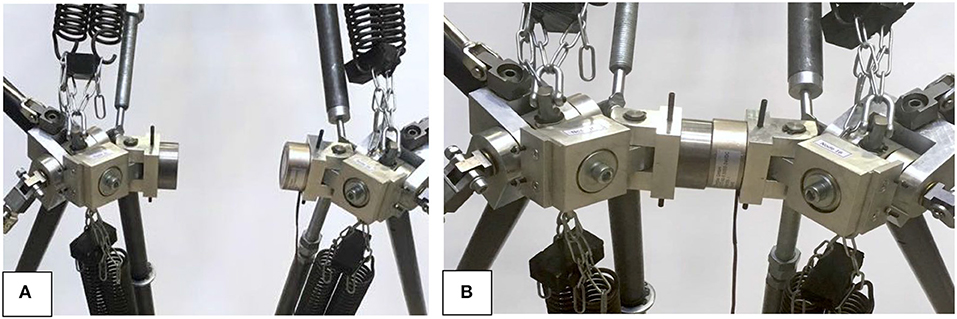
Figure 4. Electromagnets at end-nodes of the tensegrity structure halves prior to midspan connection (A) and after midspan connection (B).

3. Testing Methodologies

Presented in this work are three control phases and the respective goals of the tensegrity footbridge. Firstly, deployment involves the greatest shape change of all the phases. The next phase, self-stress, is important once the two halves of the structure are connected since this determines behavior in service. Self-stress sets the structure in an optimal configuration with respect to geometric and internal forces. In the last phase, the goals are to ensure that internal forces are within elastic limits and that structural deflections are acceptable. This paper focuses on control algorithms for the first and second phases, deployment and self-stress.

Control-commands, that which moves the tensegrity structure, are governed by the minimization of a cost function based on maximum element forces and minimal nodal distances between design and deployment. The algorithm for finding control-commands includes a stochastic-search method, Probabilistic Global Search Lausanne (PGSL), and dynamic relaxation (DR).

3.1. Feedback Method Compared With Empirically Predetermined Control Commands

Feedback for midspan connection that was previously developed by Veuve et al. (2015) used measurements. Simulation of the deployable tensegrity structure did not include sliding-friction of continuous-cables over joints and uncertainties due to construction. Deployment control-commands are carried out while avoiding strut contact and over-stressing of elements. Cable-length changes are a maximum of 5 [cm] per control command.

A sensitivity analysis is executed to study effects of the number of feedback cycles on deployment. Change in overall structure length is used for testing feedback cycles are 1 [cm], 2 [cm], 8 [cm], 20 [cm], and 50 [cm] corresponding to 160, 80, 20, 8, and 4 cycles. The first two lengths for the feedback cycle are too small given the variation in position of each of the five end-nodes of the structure. The greatest improvement in deployment is observed between the overall structure length change between 50 [cm] and 8 [cm] which corresponds to four-cycle and twenty-cycle feedback processes.

The empirically-determined deployment cable-length changes lengths of cables at different rates in order to avoid strut contact and bending of the struts. Prior to midspan connection, the final 50 [cm] of cable lengthening is carried out uniformly from all actuators. When these commands are used with the feedback method, measurements are compared with simulation values for the same length of cable relaxation at the break in each cycle.

Since there are empirically-determined commands and previous behavior of the structure is known, the feedback method is similar to PID control discussed by Astrom and Hagglund (1984) and Han (2009). PID control was chosen due to its long-standing usefulness and efficiency for closed-loop control of large structures. No fine adjustment of PID setting was required since no control loop was faster than approximately 10 s. Equation (1) shows the adjustment factor ($\overline{E_{p,k,i}}$) for each end-node (i) between measurements (p_{M, k, i}) and simulated positions (p_{S, k, i}) of the current deployment step, k. When step number is greater than k = 1, the adjustment factor, $\overline{E_{p,k,i}}$, is the mean of E_{p, k, i} and E_{p, k−1, i} (Equation 1). Adjustment factors are limited to twice the cable-length-change shown in the empirically-determined set of control commands

$\begin{array}{cc}\overline{E_{p,k,i}}=\left\{\begin{array}{cc}\frac{p_{M,k,i}-p_{S,k,i}}{p_{M,k,i}}& \text{ if }k=1\\ \frac{E_{p,k-1,i}+E_{p,k,i}}{2},& \text{ if }k>1\end{array}\right\}& (1)\end{array}$

This process was repeated for each global coordinate direction x (longitudinal), y (translational), and z (vertical), and tension in each continuous cable (E_{u, k, i}), shown in Equation (2). The adjustment factor ($\overline{E_{u,k,i}}$) for each end-node (i) between measured tension values (u_{M, k, i}) and simulated tension values (u_{S, k, i}) of the current deployment step, k. When step number is greater than k = 1, the adjustment factor, $\overline{E_{u,k,i}}$, is the mean of E_{u, k, i} and E_{u, k−1, i}.

$\begin{array}{cc}\overline{E_{u,k,i}}=\left\{\begin{array}{cc}\frac{u_{M,k,i}-u_{S,k,i}}{u_{M,k,i}}& \text{ if }k=1\\ \frac{E_{u,k-1,i}+E_{u,k,i}}{2},& \text{ if }k>1\end{array}\right\}& (2)\end{array}$

3.2. Path-Planning Method

The path-planning method consists of three parts, the path-planning algorithm (RRT*-connect), even cable-length changes, and feedback search. Table 1 shows the overall length of the structure during deployment and the stages used in this method. The first stage using RRT is applied to the structure from the folded state to 100 [cm] length, a position that no longer is at risk for element collision. The overall length to end RRT*-connect is determined by measurement and simulation to ensure strut elements do not risk contact following subsequent commands. Next, all cables are deployed evenly until approximately 180 [cm] which is near midspan connection. The overall length to end the even deployment of active cables is until the first node pair is within approximately 5 [cm] of connection and this is measured from tests. Lastly, the feedback search connects end-nodes of each half of the tensegrity structure sequentially.

TABLE 1

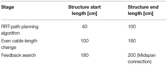
Table 1. Stages of the path-planning method and corresponding structure deployment length.

3.2.1. Simulation of the RRT*-Connect Algorithm for the Tensegrity Structure

The following section presents the simulation of the RRT*-connect algorithm developed for the deployable tensegrity structure. Boundaries of the search space are defined by spaces occupied by current positions of struts and cables to avoid element collision and over-stress. Collision avoidance involves preventing that two bars develop unwanted contact forces when the structure is in its folded and near-folded states. The RRT*-connect algorithm includes the dynamic relaxation model of the tensegrity structure to check if the newly proposed deployment point, q_rand, crosses through a structural element. In the model, elements are defined by two nodes and by an index as to which nodes are connected to form elements.

Since the elements move in space and relative to each other during deployment, the path is discretized into a sequence of intermediate steps for collision and over-stress avoidance. For each step, an initial point and a target point are defined as well as the search space populated with points defined by Voronoi regions of the search space. A sensitivity analysis is completed for the number of steps of the RRT*-connect algorithm where the distance to the next point in the tree, ϵ, is a maximum value of 5 [cm]. This value is confirmed by the increment determined for the sensitivity analysis for the feedback algorithm.

Collision and overstress avoidance of nodes that are not end-nodes, called interior nodes, restrict movement to the deployment trajectory of end-nodes (Figure 5A). The rectangle defines the outer most boundary of the search space. Depth of the 2D-section shows path around boundaries possible in three dimensions. Trees grown from the initial interior node to the target interior node are shown in black and gray respectively. Control commands of all active cables are the variables of the RRT*-connect algorithm and the objective is expressed as the Euclidian coordinates of the end-nodes. Variables and objectives are related by applying cable-length changes of the control commands to the dynamic relaxation model of the tensegrity structure to find new nodal positions.

FIGURE 5

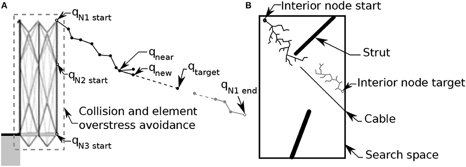
Figure 5. Path of an end-node is shown for collision and over-stress avoidance. A sample longitudinal 2D-section of the tensegrity structure (A) shows the RRT*-connect algorithm navigation around structural elements possible in three dimensions. A schematic of the RRT*-connect algorithm notation for one step (B). Successful points for two trees, one from the start point and one from the end, are shown in black and gray respectively.

The tree is extended from the start point by adding a new vertex in an optimal direction based on the search space using a greedy algorithm at a maximum radius from the current vertex. In Figure 5B, a new successful point, q_new, added to the tree connected to q_near. The new point is in the optimal direction, q, at a distance, ϵ, which is the control command and the variable of the RRT*-connect algorithm.

The goal is to find a feasible path between a folded and deployed state of the tensegrity structure. Using the methodology of RRT-connect (Xu et al., 2014), two search trees are created, one at the start point and one at the target point (Figure 6). Successful points for two trees, one from the initial point and one from the target, are shown in black and gray respectively in Figure 5B. When feasible points have been found, primary and secondary roles of the two trees are exchanged to allow both trees to extend into the search space.

FIGURE 6

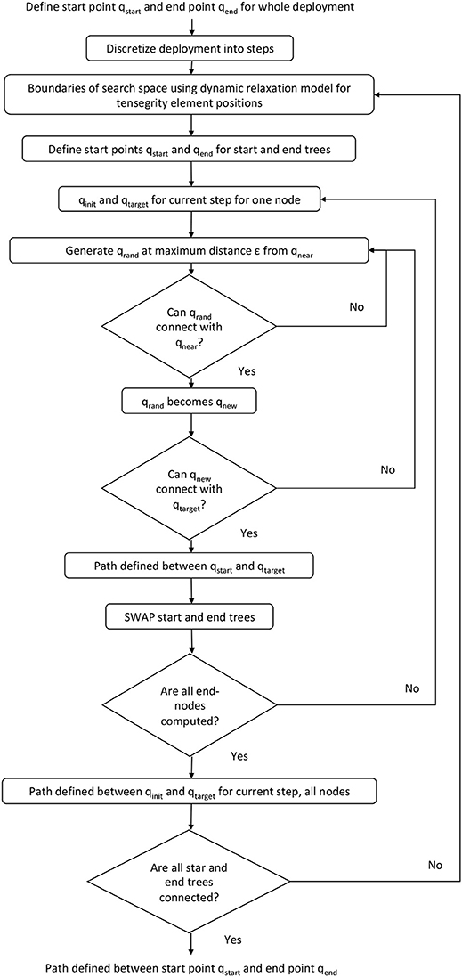
Figure 6. RRT path-planning procedure for movement of the tensegrity structure.

3.2.2. Application of RRT*-Connect Algorithm on the Tensegrity Structure

Although it is possible to implement RRT*-connect for complete deployment of the tensegrity structure, the benefits for collision and element over-stress avoidance are highest when the structure is in its folded state. RRT*-connect is implemented in simulation with struts having a diameter 2 [cm] and cables having a diameter 1 [cm] larger than that of the element. This margin is intended to account for construction and modeling uncertainty and is determined by the drift of 1 [cm] observed in the end-nodes when using the RRT*-connect algorithm on the near-full-scale tensegrity structure. For new proposed points q_rand for nodes, geometrical limitations due to bars and force limitation of elements are checked. If these limitations are not exceeded and no collisions occur, the proposed value of q_rand is retained as q_new.

Control commands for the first deployment phase were constrained to result in movement only in the direction of deployment and maximum distance, ϵ, to the next node in the tree. Twenty tests were executed for each step of the RRT*-connect algorithm. Average control commands were calculated and simulated with the dynamic relaxation model of the tensegrity structure to determine feasibility. Simultaneously, the RRT algorithm were run for five end-nodes to move from their original points in the folded configuration to their respective target points.

In the folded state, active cables have a higher tension value and the five active cables have more similar tension values than in the deployed state. Additionally, implementing RRT*-connect throughout the entire deployment lengthens execution time due to calculation when the benefits of path-planning are not utilized. Therefore, an incremental active cable-length change directly correlates to the movement of that given end-node without greatly affecting positions of other end-nodes. The first phase of deployment with the RRT*-connect algorithm involves the assumption that within each 5 [cm] segment per active cable (see section 4.2), is locally linear and independent of other active cables. Actuation of each active cable is coupled following the first phase of the deployment process.

Recall that the variable of the RRT*-coonect algorithm is active cable-length change to move the structure from q_near to q_new for each end-node. The objective is expressed as Euclidean nodal coordinates of the target using the variable value of cable-length change. Since the RRT algorithm discretizes the trajectory, the path between q_near and q_new is linearized. The vector of the trajectory, ϵ, to move from the nearest node, q_near, to target node, q_target, has a rotation expressed in quaternions (Equation 3) proportional to the end-node due to an active cable-length change (Equation 4), shown in Equation (5). H_step and H_act are the set of quaternions (for each step and complete deployment trajectory respectively) for a given rotation written in a linear combination where a, b, c, and d are real numbers and î, ĵ, $\widehat{k}$, and $\widehat{1}$ are the quaternion in the complex plane. The following equation is applied separately to all five end-nodes.

$\begin{array}{cc}\begin{array}{r}{H}_{\mathrm{\text{step}}}=a_{\mathrm{\text{step}}}·1+b_{\mathrm{\text{step}}}·î+c_{\mathrm{\text{step}}}·ĵ+d_{\mathrm{\text{step}}}·\widehat{k}\end{array}& (3)\end{array}$

$\begin{array}{cc}\begin{array}{r}{H}_{\mathrm{\text{act}}}=a_{\mathrm{\text{act}}}·1+b_{\mathrm{\text{act}}}·î+c_{\mathrm{\text{act}}}·ĵ+d_{\mathrm{\text{act}}}·\widehat{k}\end{array}& (4)\end{array}$

$\begin{array}{cc}\begin{array}{r}\frac{a_{\mathrm{\text{step}}}}{a_{\mathrm{\text{act}}}}=\frac{b_{\mathrm{\text{step}}}}{b_{\mathrm{\text{act}}}}=\frac{c_{\mathrm{\text{step}}}}{c_{\mathrm{\text{act}}}}=\frac{d_{\mathrm{\text{step}}}}{d_{\mathrm{\text{act}}}}\end{array}& (5)\end{array}$

Therefore, linear distance between Euclidean coordinates of q_near to q_target equates to the control command for active cable-length change of the given end-node, l_actuation (Equation 6) with a maximum value of ϵ.

$\begin{array}{cc}\begin{array}{r}{l}_{\mathrm{\text{actuation}}}=\sqrt{{(x_{q_{\mathrm{\text{target}}}}-x_{q_{\mathrm{\text{near}}}})}^2+{(y_{q_{\mathrm{\text{target}}}}-y_{q_{\mathrm{\text{near}}}})}^2+{(z_{q_{\mathrm{\text{target}}}}-z_{q_{\mathrm{\text{near}}}})}^2}\end{array}& (6)\end{array}$

3.2.3. Even Cable-Length Changes

For the second phase, control commands of this method are all even cable-length changes for all end-nodes from an approximate structural length of 100 [cm] to 180 [cm]. There is no risk of element collision or overstress beyond 100 [cm] as observed experimentally and through simulations. At the end of this phase, the end-nodes at the top of each half of the structure are closer to one another, approximately 7 [cm], than the end-ends at the bottom prior to the phase for midspan connection.

3.2.4. Search for Midspan Connection

The last phase uses a search for control commands to achieve midspan connection. Although each node is connected sequentially, cable-length changes occur in all active cables for successful connection at midspan of one pair of end-nodes.

Similar to the algorithm described by Veuve et al. (2017), the objective is to reduce the distance between the selected pair of end-nodes to zero, thus establishing a connection. The maximum incremental movement of active cables is set at 1 [cm] so that the goal is not surpassed. Measurements of the current pair of end-nodes are compared with the simulation (using the PGSL search algorithm) of the tensegrity structure to determine cable-length changes for the current step. Previous work tested all combinations of active cable-length changes and implemented the case that reduced the most distance between a pair of end-nodes.

This procedure is repeated for the connection of every pair of end-nodes. Since the measured end-node positions are never exactly the same, the control commands computed by the simulation also changed each test. The procedure of the search for midspan connection is repeated thirty times, each test taking the cumulative average of the control commands determined by the simulation of all tests. Convergence of control commands is observed after approximately eight tests.

3.3. Algorithms for Self-Stress

The shape of the structure after midspan connection is irregular and not necessarily aligned between the two supports. In Figure 7A the structure is above the reference line whereas in Figure 7B, the structure is centered. Node positions are more similar to the design configuration after self-stress than before. Irregular configurations risks unexpected joint angles and undesirable internal forces. Two self-stress algorithms for shape correction are studied restore configuration of the tensegrity structure regardless of position after midspan connection.

FIGURE 7

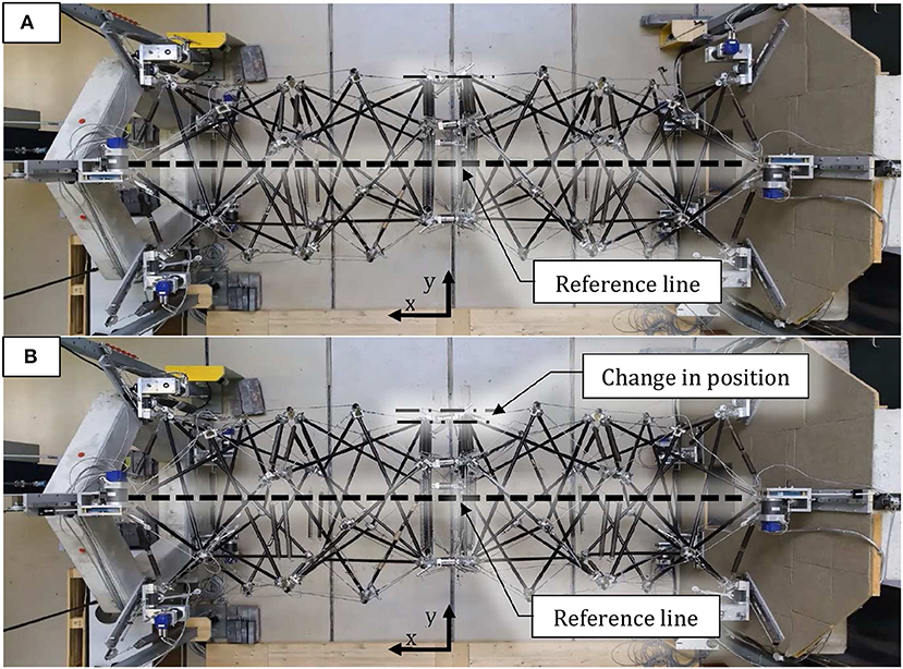
Figure 7. View from above of the tensegrity structure (A) post midspan connection and (B) after an initial self-stress imposed. In (B), the reference line becomes the center-line of the structure.

In addition to providing strength and stability to the structure, goals during self-stress are to remove slack in cables and to align the structure. Configuration has been verified using an optical tracking system with eight infrared cameras, four on each bridge support. Cable tension has been measured using a handheld spring-actuated cable tension-measuring device. The self-stress phase improves the tensegrity structure node positions to obtain a well-aligned, uniform shape that is close to the design configuration. The PGSL search algorithm was implemented to find control commands for midspan connection of the two bridge halves. Although many algorithms have been investigated, such as those proposed by Papalambros and Wilde (1989), algorithms based on two types of constraint are investigated in this paper.

The cost function to be minimized includes a term that represents the distance between the end-nodes on each bridge half. Figure 8 shows a flow chart of the algorithm for self-stress. Two versions of this algorithm, hard-constraint and soft-contraint, that have been built on previous work (Veuve et al., 2015) are evaluated. Algorithms successfully prescribe cable-length changes to result in self-stress values that are close to the design configuration.

FIGURE 8

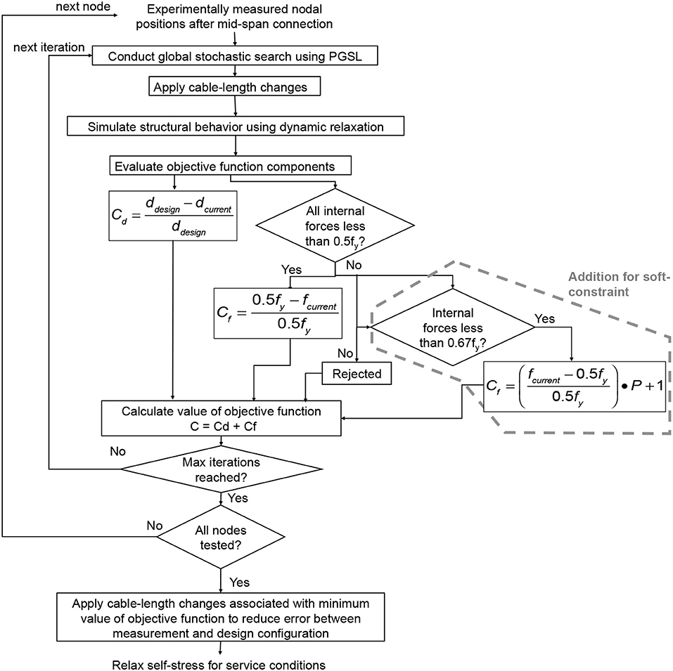
Figure 8. Procedure for multi-criteria objective function within the stochastic search algorithm, PGSL. Cable-length changes govern the objective function value.

Both algorithms involve the computation of an objective function value from the normalized nodal position distances and the normalized element internal forces. This configuration is evaluated based on the two criteria of the objective function; current distance away from design configuration in millimeters, (difference between d_current and d_design), and internal force limits. A hard-constraint algorithm, called the initial algorithm, rejects the element internal force in kilonewtons,f_current, if the axial forces are greater than half of the material yield value, 0.5f_y, for the element cross sectional area. This value is conventionally taken for the purposes of experimental work. A soft-constraint algorithm adds a condition where a penalty factor, P, of value 1.25 if the element internal force is greater than 0.5f_y and less than 0.67f_y, is applied to the surcharge of the objective function in PGSL.

The simulation ends after 400 iterations of PGSL were reached for all midspan nodes. This number was fixed a-priori to be 400 since it was observed that the value of the objective function did not change the overall result beyond 300 iterations.

Components of the objective function are expressed as follows:

$\begin{array}{cc}\begin{array}{r}{C}_d=\frac{d_{\mathrm{\text{design}}}-d_{\mathrm{\text{current}}}}{d_{\mathrm{\text{design}}}}\end{array}& (7)\end{array}$

If f_current < 0.5f_y, then

$\begin{array}{cc}\begin{array}{r}{C}_f=\frac{0.5f_y-f_{\mathrm{\text{current}}}}{0.5f_y}\end{array}& (8)\end{array}$

If 0.5f_y < f_current < 0.67f_y, then

$\begin{array}{cc}\begin{array}{c}{C}_f=\left(\frac{f_{\text{current}}-0.5f_y}{0.5f_y}\right)·P+1\end{array}& (9)\end{array}$

If f_current > 0.67f_y, then the control solution is rejected

The objective function is taken to be the total cost, C, which is the cost of the distance component, C_d, added to the axial force component, C_f (see Equations 8 and 9). The algorithms are intended for the full-structure in the design configuration with cables successfully having their prescribed self-stress values.

$\begin{array}{cc}\begin{array}{r}C=C_d+C_f\end{array}& (10)\end{array}$

The goal of both algorithms is to find a state of self-stress for the structure so that it is in the configuration closest to the design specification. Element axial forces must be relaxed to prepare for the service phase. Although nodal positions of the structure while in service may not be exactly as designed, the structure benefits from the self-stress phase that corrects for mis- aligned elements after midspan connection.

4. Results

4.1. Feedback Method

Testing of the feedback method for four cycles and twenty cycles is completed twenty times each. Figure 9 shows results from the average of corrected and uncorrected control commands with four cycles (a) and twenty cycles (b). There are no cycles when there is no feedback. Commands are executed sequentially without the check that occurs at the end of a cycle. The number of control commands is shown on the horizontal axis and the average actuation cumulative cable-length change of continuous cables shown on the vertical axis. The average cumulative cable-length change is shown over twenty tests without feedback control (gray dashed line) and with feedback control (black line). Error bars show two standard deviations, 2σ, for cable-length change commands per control command over twenty tests. When there are only four cycles, predetermined control-commands have a greater cumulative cable-length change than feedback-control (see Figure 9A). When the number of feedback cycles is increased, feedback control successfully arrives at the deployed state in fewer control commands than the four-cycle feedback control (see Figure 9B). Since the control commands without feedback are not modified in cycles, the average cumulative cable-length changes are the same for Figures 9A,B).

FIGURE 9

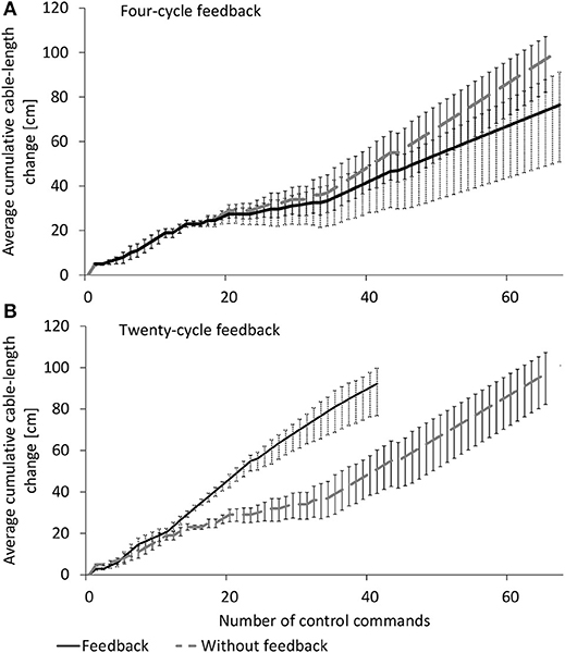
Figure 9. Average cumulative cable-length change for measured deployment with and without feedback control in (A) four cycles and (B) twenty cycles of equal structure deployment length for twenty trials. Two standard deviations of end-node position error are shown. Cable-length changes without feedback (gray dashed line) are the same for (A,B).

The number of cycles for the feedback method results in the shortest possible time of deployment considering calculation time and benefit of feedback control as shown in Equation 11. Variable t_{optimal,Noptimal} is the minimum time of deployment for the optimal number of cycles, N_optimal, t_{calc,Noptimal} is the time of calculation for a given number of cycles, and t_{feedback,Noptimal} is time due to deployment with feedback with a given number of cycles.

$\begin{array}{cc}\begin{array}{c}{t}_{\text{optimal},N_{\text{optimal}}}=\min \left(t_{\text{calc},N_{\text{optimal}}}+t_{\text{feedback},N_{\text{optimal}}}\right)\end{array}& (11)\end{array}$

As the number of cycles increases, the time of deployment decreases nonlinearly with decay as more cycles are introduced. Between four, ten, and twenty cycles, twenty cycles significantly reduces deployment time. However between twenty and one-hundred cycles, there is very little reduction of deployment time.

In contrast, calculation time increases with a polynomial complexity of ${O}(n)$. Despite there being nested loops to calculate mean overall structural length that determines when the structure has reached the next cycle, the length of the loops are independent of the number of cycles and thus not taken into consideration for complexity of the calculation. With the increasing calculation time and the decaying benefit of feedback control, the optimal number of cycles for the tensegrity structure is twenty.

Sources of uncertainty are the effects of geometry not present in simulation, such as eccentricities due to joint construction. Despite these uncertainties, modification of future deployment control-commands acting on cable-length changes based on the comparison between design shape and measured position moves the structure in the correct direction. Increasing the number of stages decreases real-time response time of the structure, resulting in smaller and regular changes compared with fewer stages.

Figure 10 shows a comparison of elapsed time of deployment trajectories without feedback (dashed gray line) and with feedback for four (dashed black line) and twenty (black line) cycles. The horizontal axis shows deployment time in seconds and the vertical axis is the overall structure length in centimeters. The standard deviation of 95%, 2σ, is shown in gray for each line. Error bars indicate the maximum and minimum end-node positions in the direction of deployment. Time of deployment is successfully reduced by introducing four-cycle and twenty-cycle feedback control compared with deployment without feedback. Fastest deployment occurs with twenty cycles and reduces elapsed time prior to midspan connection by approximately 50% compared with deployment without feedback.

FIGURE 10

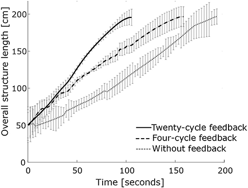
Figure 10. Comparison of deployment trajectories for twenty tests without feedback, four-cycle feedback, and twenty-cycle feedback. Two standard deviations of end-node position error are shown.

Due to self-weight of the structure, cables on the upper face of the structure are more in tension, making actuation of these cables more influential on structure shape. The feedback-controlled deployment trajectory successfully reduces deployment time compared with the original deployment trajectory.

Feedback control and sensing of the tensegrity structure is helpful for development toward a deployment trajectory that adapts to uncertainties. Cable-length changes using the difference between measurement and simulation does not create new deployment sequences. Instead, control commands for each continuous cable are modified by a scalar correction factor that is unique to each continuous cable. This computes faster than searching through the solution space for a new control command. The optimization mentioned previously in this work shows no improvement when the number of cycles is greater than twenty. Feedback with over fifty cycles is affected by variation in longitudinal positions of each end-node and therefore not implemented.

Correction factor values from several cycles of deployment tests vary within a small range due to non-repeatability of the tensegrity structure movement. Modification of deployment control-commands based on comparisons between design shape and measured position successfully results in a more efficient deployment trajectory. However, there is no assurance of collision avoidance. This leads to another strategy which is presented next.

4.2. Path-Planning Method

The path-planning method is compared with the feedback method to assess quality of movement. Least-squares is used to evaluate deployment trajectories. A trajectory curve is discretized into linear segments with an optimal discretization given sensitivity analysis which is every 5 [cm]. The summation is taken of the squared shortest distance from each measurement point to the linear segment. Low values of least-squares means points follow a deployment trajectory. Least-squares minimizes the sum where the residuals are the differences between measurement points and the fitted values. Since the curve is discretized and linearized, this fitted value creates the fitted curve of the deployment trajectory.

Applying the methodology for deployment trajectory, Figure 11 shows simulated and measured deployment trajectories for the feedback method and the path-planning method. Deployment ends just prior to midspan connection where the node pair at the top of the structure is approximately 5 [cm] apart, and thus not all nodes are shown to full deployed length. End-node positions are shown comparing measurement and simulation of the feedback method (a). End-node positions are also shown comparing measurement and simulation of the path-planning method (b). Hollow markers indicate simulated end-node positions and filled markers indicate measured end-node positions. Measured and simulated end-node positions are marked every 5 [cm] and average deployment trajectories are shown with a continuous line. Distances between the trajectory and the least-squares fitted curve are less for the path-planning method than with the feedback method.

FIGURE 11

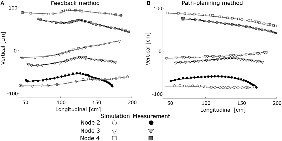
Figure 11. End-node positions are shown from simulation and measurement of (A) the feedback method and (B) the path-planning method. Three end-nodes are shown.

Although simulation and measurement for the feedback method show similar trends, end-node positions are not significantly correlated. For the path-planning method, simulation and measurement successfully show similar trends. Two of the three nodes are significantly correlated at the end of deployment for the path-planning method. Simulation of the path-planning method does not involve real-time feedback using measurements, thus only some end-node simulations and measurements are significantly correlated. Error in positions of paired end-nodes during the midspan connection of the two halves of the tensegrity structure is successfully reduced to approximately 1 [cm] (average over twenty tests) through feedback control at midspan.

For both simulation and measured positions, the path-planning method successfully reduces variation compared with the feedback method. Using the same motor speed for deployment as used by Veuve et al. (2016), the new deployment trajectory successfully enables deployment with greater than 68% reduction in deployment time. During deployment of the tensegrity structure, eccentricities at nodes incur shifts in nodal positions, as shown in Figure 11A at a structure length of approximately 120 [cm]. Node details are not modeled in the simulations. Feedback search in the last phase of deployment successfully resolves this difference and this process requires real-time comparison of simulation and measurements.

Although incorporating feedback control within the RRT*-connect is attempted, the resulting deployment of the first 60 [cm] of the structure was slower than without feedback. Real-time feedback is thus only involved in the last phase of the path-planning method. The measured nodal positions are compared to the simulated nodal positions to modify the deployment trajectory. However, measured nodal positions and element stresses are more consistent with the simulation when the structure is folded. Therefore there is minimal benefit to incorporating feedback of measured position for the RRT*-connect algorithm for this phase of deployment. Additionally, this comparison between measurement and simulation added approximately 20 s per RRT path-planning step of 5 [cm] and computational complexity to the deployment sequence.

4.2.1. Evaluation of Deployment Schemes

Table 2 shows a comparison of least-squares in [cm] of end-joint positions determined by simulation of the feedback method and the path-planning method compared with the ideal trajectory. The feedback method is consistently more irregular than the path-planning method for simulation and measurement. Variance of least-squares values from measurements from the path-planning method are lower than that of the feedback method.

TABLE 2

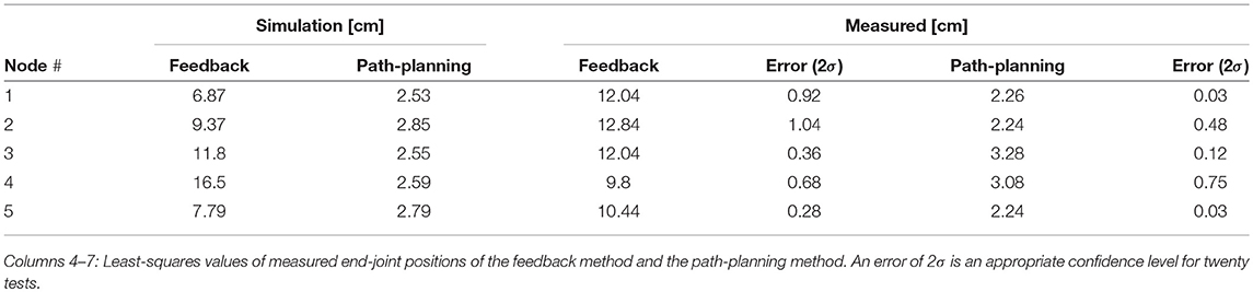
Table 2. Columns 2–3: Least-squares values of end-joint positions from simulations of the feedback method and the path-planning method.

4.3. Algorithms for Self-Stress

The goal of the self-stress algorithm is to realign the structure between the supports. To study the effects of self-stress-control-commands, element internal forces after midspan connection and after applying the initial self-stress algorithm are compared in Figure 12A. Results from a soft-constraint algorithm are presented in Figure 12B. The vertical axis is the axial force [kN] in elements where tension is positive. Element numbers are shown on the horizontal axis.

FIGURE 12

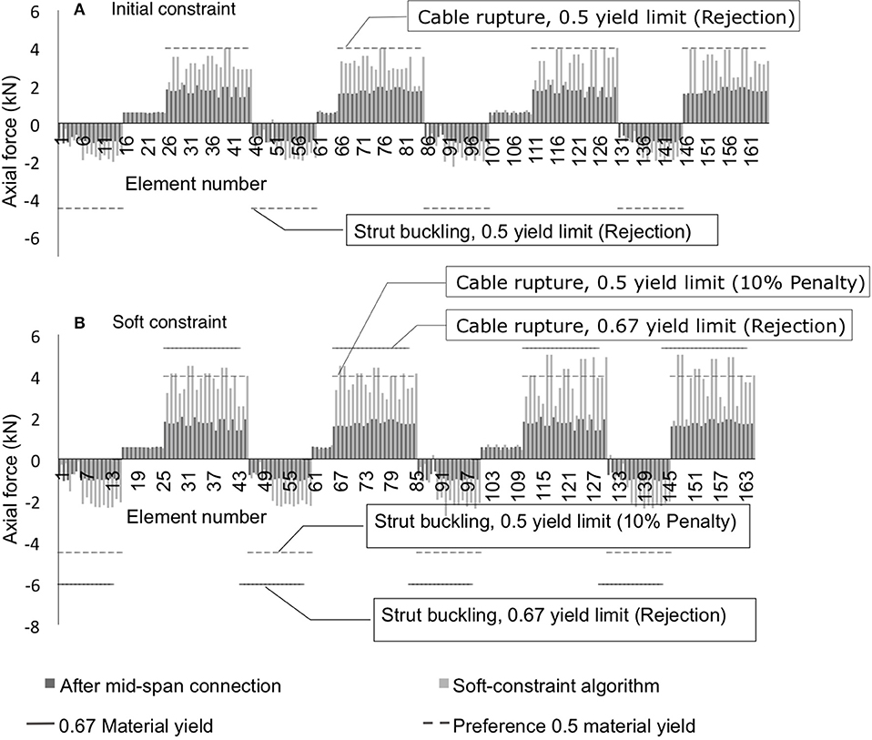
Figure 12. Comparison of simulated element internal forces using an initial self-stress algorithm (A), and soft-constraint self stress algorithm (B). The dark gray bars show the original element forces and the light gray bars show the element forces with application of each constraint algorithm.

Dark gray vertical bars indicate element internal forces after midspan connection. Light gray vertical bars denote results of the self-stress search function. Struts can sustain an axial force of 9 [kN] in compression whereas cables are able to resist 8 [kN] in tension. Limits shown with a horizontal dash line are set to be half of the material yield limit as described earlier. Since the tensile limit of struts is 31 [kN], it is not shown.

Using the initial algorithm, axial force in discontinuous cables increases with the application of the self-stress. Continuous cables that run from the end-nodes to the middle support nodes increase in tension whereas the remaining continuous cables decrease in tension. The active cables The minimum cable force is 1.33 [kN] and the maximum is 3.98 [kN] and the final value for C is 57.5 (Equation 10).

With the soft-constraint algorithm, axial forces in some cables increase by up to a factor of eight. Some of the continuous cables exceeded the soft constraint of 0.5f_y in the solution selected by the algorithm, probabilistic global search Lausanne (PGSL). The cable tension values are more uniform throughout the structure than with the initial algorithm and just after midspan connection. Since the structure has been designed for ideal near-uniform axial forces, behavior of the structure is expected to be more predictable when element forces are uniform. This results in a value for C of 50.6 (Equation 10). The minimum cable force is 2.53 [kN] and the maximum is 5.02 [kN]. Since the goal is to minimize the value of the objective function, which is the difference between the post midspan connect and design values for element forces and nodal positions, the soft-constraint self-stress algorithm is more successful than the initial algorithm for attaining uniform self-stress.

For each structural node, Figure 13 shows the distance to the design position after midspan connection, after applying the initial algorithm, and after applying the soft-constraint algorithm. By permitting some cables to carry tension above 0.5f_y, the soft-constraint algorithm successfully reduces the distance between measurement and design configuration.

FIGURE 13

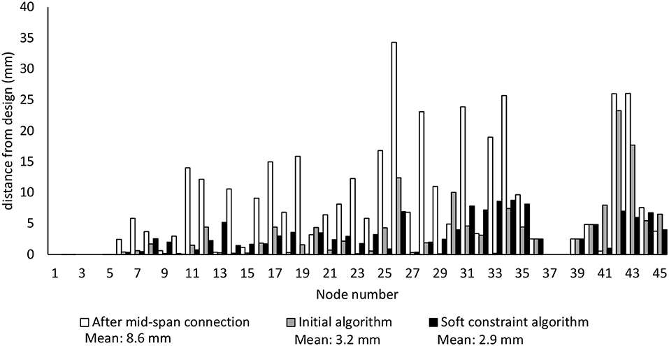
Figure 13. Comparison of simulated nodal position distances [mm] after midspan connection, after application of the initial self-stress algorithm, and after application of self-stress soft-constraint algorithm.

When the structure is put in service, self-stress values will be relaxed to a range of 12.5–20% of the yield stress (Rhode-Barbarigos et al., 2010a). End-node vertical displacements have been simulated when self-stress in active cables is lowered by approximately 20%. Implementing the feedback method with self-stress results in an average measured vertical end-node settlement of 5 [cm]. Implementing the path-planning method with self-stress results in an average measured vertical end-node settlement less than 1 [cm].

Active cables with no tension present two challenges, they do not respond to cable-length changes and more work is required by other active cables to move the structure. Therefore, if control commands result in active cables having no tension, movement of the structure toward the design configuration is a challenge which is the observation of deployment using the feedback method. However, the path-planning method maintains nodal positions and element stress values closer to the design configuration throughout deployment so that with a reduction of self-stress, the structure vertically settles less than with the feedback method.

5. Discussion

This section summarizes the generality and limitations of results found from this work.

5.1. Feedback Method

Feedback control developed for movement of the tensegrity structure is already widely applied in other situations. The novelty of this work is the real-time comparison of tests with simulations (model-based) of a full-scale deployable tensegrity structure. Re-use of this algorithm would be useful for other structures that deploy along several degrees of freedom. Even though control in real-time is computationally expensive, efficient deployment trajectories for the tensegrity structure provide the opportunity to increase the deployment speed without over-stressing elements.

The optimal number of cycles to reduce time of deployment is dependent on calculation time and benefit due to feedback for the given structure. Although the optimum for the tensegrity structure is twenty cycles, it is likely to be different for another structure. These factors are generalizable for any structure.

Differences between measurement and simulation are unavoidable. Although cable tension is checked to prevent over-stress, it is nodal position that is the primary feedback criterion. This methodology may be used on other structures involving complex movement.

Challenges of feedback control on the tensegrity structure are that maximum and minimum adjustment factors must be set on cable-control commands to prevent the structure from being over-stressed. When magnitude of nodal coordinates vary, calculation of the feedback coefficient does not affect large and small magnitude values equally. Continuous control is not the optimal choice since time of calculation increases and the increased benefit is low for the tensegrity structure.

Although the incremental movement using the feedback method is small at a length of 5 [cm], there is no assurance for collision and overstresss avoidance which add bending stresses as well as plastic deformation in struts. Scaling of control commands is based on already executed commands to compare simulation and measurement. Assuming deployment of the structure is slow (time greater than ten times first natural frequency) and considered to respond with quasi-static behavior, deriving equations of motion to predict positions of elements in the future using measurements is not relevant. To improve on collision and overstress avoidance, the path-planning method is proposed.

5.2. Path-Planning Method

Using the path-planning method when the structure is nearly folded, less variability is observed in structural movement than when the structure is near midspan connection. Therefore, the path-planning method for deployment through complex search spaces can be applied to deployment of other structures. When accuracy is required at the expense of longer time of deployment, control-command calculation could compare measurement and simulation in real-time.

The path-planning method uses a search for control commands to achieve midspan connection. Targeting restricted phases of deployment for small-increment search is useful to save energy and time rather than using the search method throughout deployment. This is applicable to deployment of other complex deployable structures. Determining phases of deployment requires previous knowledge which can be stored as training data. Given a new structure with unknown behavior, path-planning can be implemented. Once training sets are determined, control-command smoothing helps improve effectiveness and lowers deployment time.

Use of the path-planning method involves the assumption that the folded configuration is known precisely. In situations where this is not the case, image-recognition methods may be useful to improve knowledge of the folded configuration thus ensuring the effectiveness of path-planning.

5.3. Algorithms for Self-Stress

Similar to feedback control, algorithms for self-stress are useful for structures when there are large differences between ideal and real nodal positions following deployment. Generality is dependent on the type of active control. In cases where actuators are dispersed in the structure, self-stress algorithms would be simpler and more efficient than those used for this tensegrity structure. Actuators on this structure are placed at the supports to satisfy practical criteria associated with typical civil-engineering structures.

Future self-stressed structures may be designed to employ the benefits of a soft-constraint algorithm to optimize structure configuration. Allowing the structure to move beyond the operating range at a penalty results in several elements being stressed slightly more than allowable service levels. Before service, prestress is reduced to optimize load-carrying capacity.

6. Conclusions

The number of control cycles in feedback method should be determined according to factors contributing to time of deployment. The optimal number of cycles occurs at the shortest deployment time considering time of calculation of each cycle and time of deployment with feedback for the given number of cycles. Deployment with twenty cycles successfully reduces elapsed time by approximately 50% compared with deployment without feedback.

Advanced computing algorithms have potential to improve further the efficiency of complex deployment challenges. The path-planning method successfully enables deployment and connection at midspan with at least a 68% reduction in time compared with the feedback method, in addition to the previously mentioned reduction of elapsed time. Error in nodal positions at midspan is successfully reduced through the use of the path-planning method.

Constraint relaxation is useful for correcting nodal positions after deployment. The soft-constraint algorithm for self-stress that is described in this work successfully lowers variability of axial forces in cables as well as the discrepancy between real and ideal nodal positions. Similar to feedback control, algorithms for self-stress are useful for structures with uncertainty related to deployed nodal positions and element forces in the structure.

Author Contributions

AS developed the path-planning method for deployment and feedback and self-stress control using measurements. AS wrote the majority of the paper and conducted the research and simulations mentioned. IS was actively involved in the conception of the algorithms and wrote parts of the contribution. All authors reviewed and accepted the final version.

Funding

The research is sponsored by funding from the Swiss National Science Foundation under project number 200020_169026.

Conflict of Interest Statement

The authors declare that the research was conducted in the absence of any commercial or financial relationships that could be construed as a potential conflict of interest.

Acknowledgments

The authors would like to acknowledge Jacob Ritchie, Johanna Isaksson, and Arka Prabhata Reksowardojo for their help with simulations for this work.

References

Abrar, S., Zerguine, A., and Deriche, M. (2005). Soft constraint satisfaction multimodulus blind equalization algorithms. IEEE Signal Process. Lett. 12, 637–640. doi: 10.1109/LSP.2005.853042

CrossRef Full Text | Google Scholar

Adam, B., and Smith, I. F. (2008). Active tensegrity: a control framework for an adaptive civil-engineering structure. Comput. Struct. 86, 2215–2223. doi: 10.1016/j.compstruc.2008.05.006

CrossRef Full Text | Google Scholar

Akande, K., Iqbal, N., Zerguine, A., and Chambers, J. (2016). Normalised frequency-domain soft constraint satisfaction multimodulus blind algorithm. Electr. Lett. 52, 239–241. doi: 10.1049/el.2015.2845

CrossRef Full Text | Google Scholar

Akgün, Y., Gantes, C. J., Sobek, W., Korkmaz, K., and Kalochairetis, K. (2011). A novel adaptive spatial scissor-hinge structural mechanism for convertible roofs. Eng. Struct. 33, 1365–1376. doi: 10.1016/j.engstruct.2011.01.014

CrossRef Full Text | Google Scholar

Aldrich, J. B., and Skelton, R. E. (2003). “Control/structure optimization approach for minimum-time reconfiguration of tensegrity systems,” in Smart Structures and Materials 2003: Modeling, Signal Processing, and Control, Vol. 5049, ed R. C. Smith (San Diego, CA: SPIE), 448–459.

Google Scholar

Amendola, A., Carpentieri, G., de Oliveira, M., Skelton, R., and Fraternali, F. (2014). Experimental investigation of the softening stiffening response of tensegrity prisms under compressive loading. Compos. Struct. 117, 234–243. doi: 10.1016/j.compstruct.2014.06.022

CrossRef Full Text | Google Scholar

Ashwear, N., and Eriksson, A. (2017). Vibration health monitoring for tensegrity structures. Mech. Syst. Signal Process. 85, 625–637. doi: 10.1016/j.ymssp.2016.08.039

CrossRef Full Text | Google Scholar

Astrom, K., and Hagglund, T. (1984). Automatic tuning of simple regulators with specifications on phase and amplitude margins. Automatica 20, 645–651. doi: 10.1016/0005-1098(84)90014-1

CrossRef Full Text | Google Scholar

Averseng, J., and Dubé, J. (2012). Design, analysis and self stress setting of a lightweight deployable tensegrity modular structure. Proc. Eng. 40, 14–19. doi: 10.1016/j.proeng.2012.07.048

CrossRef Full Text | Google Scholar

Bel Hadj Ali, N., Rhode-Barbarigos, L., and Smith, I. F. C. (2011). Analysis of clustered tensegrity structures using a modified dynamic relaxation algorithm. Int. J. Solids Struct. 48, 637–647. doi: 10.1016/j.ijsolstr.2010.10.029

CrossRef Full Text | Google Scholar

Bel Hadj Ali, N., Sychterz, A. C., and Smith, I. F. (2017). A dynamic-relaxation formulation for analysis of cable structures with sliding-induced friction. Int. J. Solids Struct. 127, 240–251. doi: 10.1016/j.ijsolstr.2017.08.008

CrossRef Full Text | Google Scholar

Csölleová, Z. (2012). The analyses of triangular tensegrity prisms' pairs. Proc. Eng. 40, 74–78. doi: 10.1016/j.proeng.2012.07.058

CrossRef Full Text | Google Scholar

Domer, B., and Smith, I. F. C. (2005). An active structure that learns. J. Comput. Civil Eng. 19, 16–24. doi: 10.1061/(ASCE)0887-3801(2005)19:1(16)

CrossRef Full Text | Google Scholar

Fest, E., Shea, K., and Smith, I. F. C. (2004). Active tensegrity structure. J. Struct. Eng. 130, 1454–1465. doi: 10.1061/(ASCE)0733-9445(2004)130:10(1454)

CrossRef Full Text | Google Scholar

Gantes, C. J., Connor, J. J., Logcher, R. D., and Rosenfeld, Y. (1989). Structural analysis and design of deployable structures. Comput. Struct. 32, 661–669. doi: 10.1016/0045-7949(89)90354-4

CrossRef Full Text | Google Scholar

Han, J. (2009). From PID to active disturbance rejection control. IEEE Trans. Indust. Electr. 56, 900–906. doi: 10.1109/TIE.2008.2011621

CrossRef Full Text | Google Scholar

Islam, F., Nasir, J., Malik, U., Ayaz, Y., and Hasan, O. (2012). “RRT*-Smart: rapid convergence implementation of RRT* towards optimal solution,” in 2012 IEEE International Conference on Mechatronics and Automation, ICMA 2012 (Chengdu), 1651–1656.

Google Scholar

Kuffner, J. J. Jr., and La Valle, S. M. (2000). “Rrt-connect: an efficient approach to single-query path planning,” in Proceedings - IEEE International Conference on Robotics and Automation, San Francisco USA, Vol. 2 (San Francisco, CA) 995–1001.

Google Scholar

Liu, Y., Du, H., Liu, L., and Leng, J. (2014). Shape memory polymers and their composites in aerospace applications: a review. Smart Mater. Struct. 23:023001. doi: 10.1088/0964-1726/23/2/023001

CrossRef Full Text | Google Scholar

Moored, K., and Bart-Smith, H. (2009). Investigation of clustered actuation in tensegrity structures. Int. J. Solids Struct. 46, 3272–3281. doi: 10.1016/j.ijsolstr.2009.04.026

CrossRef Full Text | Google Scholar

Motro, R. (2011). Structural morphology of tensegrity systems. Meccanica 46, 27–40. doi: 10.1007/s11012-010-9379-8

CrossRef Full Text | Google Scholar

Motro, R., Maurin, B., and Silvestri, C. (2006). “Tensegrity rings and the hollow rope,” in IASS Symposium Beijing China (Beijing), 1–12.

Google Scholar

Papalambros, P. Y., and Wilde, D. J. (1989). Principles of optimal design-modeling and computation. Math. Comput. Simul. 31:286.

Google Scholar

Pellegrino, S. (1990). Analysis of prestressed mechanisms. Int. J. Solids Struct. 26, 1329–1350. doi: 10.1016/0020-7683(90)90082-7

CrossRef Full Text | Google Scholar

Pellegrino, S. (1995). Large retractable appendages in spacecraft. J. Spacecraft Rocket. 32, 1006–1014. doi: 10.2514/3.26722

CrossRef Full Text | Google Scholar

Pellegrino, S., and Calladine, C. (1986). Matrix analysis of statically and kinematically indeterminate frameworks. Int. J. Solids Struct. 22, 409–428. doi: 10.1016/0020-7683(86)90014-4

CrossRef Full Text | Google Scholar

Pharpatara, P., Herisse, B., and Bestaoui, Y. (2017). 3-D trajectory planning of aerial vehicles using RRT*. IEEE Trans. Control Syst. Technol. 25, 1116–1123. doi: 10.1109/TCST.2016.2582144

CrossRef Full Text | Google Scholar

Rhode-Barbarigos, L., Ali, N. B. H., Motro, R., and Smith, I. F. (2010a). Designing tensegrity modules for pedestrian bridges. Eng. Struct. 32, 1158–1167. doi: 10.1016/j.engstruct.2009.12.042

CrossRef Full Text | Google Scholar

Rhode-Barbarigos, L., Jain, H., Kripakaran, P., and Smith, I. (2010b). Design of tensegrity structures using parametric analysis and stochastic search. Eng. Comput. 26, 193–203. doi: 10.1007/s00366-009-0154-1

CrossRef Full Text | Google Scholar

Rieffel, J., Valero-Cuevas, F., and Lipson, H. (2009). Automated discovery and optimization of large irregular tensegrity structures. Comput. Struct. 87, 368–379. doi: 10.1016/j.compstruc.2008.11.010

CrossRef Full Text | Google Scholar

Schenk, M., Guest, S., and Herder, J. (2007). Zero stiffness tensegrity structures. Int. J. Solids Struct. 44, 6569–6583. doi: 10.1016/j.ijsolstr.2007.02.041

CrossRef Full Text | Google Scholar

Schlaich, M. (2003). Der Messeturm in Rostock - ein Tensegrityrekord. Stahlbau 72, 697–701. doi: 10.1002/stab.200302440

CrossRef Full Text | Google Scholar

Skelton, R. E., Adhikari, R., Pinaud, J.-P., and Chan, W. L. (2001). “An introduction to the mechanics of tensegrity structures,” in Conference on Decision and Control (Orlando, FL), 4254–4259.

Google Scholar

Smith, I. F. C., and Boulanger, S. (1994). Knowledge representation for preliminary stages of engineering tasks. Knowl. Based Syst. 7, 161–168. doi: 10.1016/0950-7051(94)90002-7

CrossRef Full Text | Google Scholar

Snelson, K. (2012). The art of tensegrity. Int. J. Space Struct. 27, 71–80. doi: 10.1260/0266-3511.27.2-3.71

CrossRef Full Text | Google Scholar

Sultan, C. (2014). Tensegrity deployment using infinitesimal mechanisms. Int. J. Solids Struct. 51, 3653–3668. doi: 10.1016/j.ijsolstr.2014.06.025

CrossRef Full Text | Google Scholar

Sultan, C., and Skelton, R. (2003). Deployment of tensegrity structures. Int. J. Solids Struct. 40, 4637–4657. doi: 10.1016/S0020-7683(03)00267-1

CrossRef Full Text | Google Scholar

Sychterz, A. C., and Smith, I. F. C. (2017). Joint friction during deployment of a near-full-scale tensegrity footbridge. J. Struct. Eng. 143, 1–10. doi: 10.1061/(ASCE)ST.1943-541X.0001817

CrossRef Full Text | Google Scholar

Tanrikulu, O., Constantinides, A. G., and Chambers, J. A. (1997). New normalized constant modulus algorithms with relaxation. IEEE Signal Process. Lett. 4, 256–258. doi: 10.1109/97.623042

CrossRef Full Text | Google Scholar

Veuve, N., Dalil Safaei, S., and Smith, I. (2016). Active control for mid-span connection of a deployable tensegrity footbridge. Eng. Struct. 112, 245–255. doi: 10.1016/j.engstruct.2016.01.011

CrossRef Full Text | Google Scholar

Veuve, N., Safaei, S., and Smith, I. (2015). Deployment of a tensegrity footbridge. J. Struct. Eng. 141, 04015021-1-04015021-8. doi: 10.1061/(ASCE)ST.1943-541X.0001260

CrossRef Full Text | Google Scholar

Veuve, N., Sychterz, A. C., and Smith, I. F. C. (2017). Adaptive control of a deployable tensegrity structure. Eng. Struct. 152, 14–23. doi: 10.1016/j.engstruct.2017.08.062

CrossRef Full Text | Google Scholar

Xu, X., Sun, F., Luo, Y., and Xu, Y. (2014). Collision-free path planning of tensegrity structures. J. Struct. Eng. 140:04013084. doi: 10.1061/(ASCE)ST.1943-541X.0000900

CrossRef Full Text | Google Scholar