Integrated Reverse Engineering Strategy for Large-Scale Mechanical Systems: Application to a Steam Turbine Rotor

Introduction

The largest proportion of electricity worldwide is produced using some kind of turbine (Steam, Hydro, Nuclear, etc.) As large density of energy flows through the turbines, the rotation speeds are extremely high, large inertia loads are developed, shaft and blade deform extensively, blades corrode and high levels of vibration occur, all leading to strong dynamic instabilities (Bavastri et al., 2008). Instability problems of turbines, especially when rotating at high speeds, can result in partial failures or system shutdown. Taking into account the size of these structures, it is necessary to avoid interruptions due to system failure, but most importantly, accidents that, in addition to financial damage, can cause serious injuries or even fatalities. This implies that detailed study and development of each turbine in various operating scenarios combined to proper maintenance, even outside the limits of normal use, are necessary.

Moreover, in the fast paces of today's most developed societies, industries are constantly trying to cope with rapid technological developments, increasing technology penetration in our everyday life, and enormous competition soaring as a result of globalization. Thus, it is imperative to minimize the time and cost, from design to production and maintenance, for a product to be developed and function as intended. So either for competition reasons, safety or reliability enhancements in addition to lack of information about a product, a widespread methodology is used, i.e., reverse engineering (Abella et al., 1994; Várudy et al., 1997; Wang et al., 2012; Ouamer-Ali et al., 2014; Dagli and Idowu, 2015). Reverse engineering is this process in which we extract knowledge, design information about the parts that make up a machine and the way they function. Issues that include developing the CAD and FE model of the examined structure, as well as experimental modal analysis procedures and the application of robust and effective computational finite element model updating techniques are taken into account.

The main objective of the present work is to demonstrate the advantages of a reverse engineering strategy applying a developed model updating computational framework (Giagopoulos and Arailopoulos, 2017) to handle large-scale linear and nonlinear models. The applicability of the framework is examined by calibrating the structural parameters of a high-fidelity FE model of a steam turbine rotor with several millions degrees of freedom, using experimentally identified modal parameters. Modal identification techniques (Eykhoff, 1974; Beck and Katafygiotis, 1998; Beck, 2011) are used to extract natural frequencies and modal damping ratios from acceleration measurements. Measured and predicted modal parameters are used to quantify the discrepancy between numerical and experimental models, defining both modal and response residuals (Giagopoulos and Arailopoulos, 2015a,b, 2016; Arailopoulos and Giagopoulos, 2016), in a single-objective optimization problem. Next, a free distribution of the non-gradient, non-intrusive optimization algorithm, Covariance Matrix Adaptation—Evolution Strategy (CMA-ES) (Hansen et al., 2003; Hansen, 2006, 2011), within Π4U framework (Hadjidoukas et al., 2015), coupled to robust and accurate FE Analysis software (DTECH, 2013) are applied in parallel computing, based on a parallel computing library, i.e., TORC (Hadjidoukas et al., 2012). Structural material model parameters, such as modulus of elasticity and density are tuned, in order to best match experimental and analytical data.

Moreover, in this work a simplified numerical model based on the updated full large-scale FE model of the steam turbine is introduced, in order to get deep insight of the rotordynamic behavior and gyroscopic phenomena of the examined rotor. The main purpose is to examine the axial, lateral, and torsional dynamic characteristics, so as to evaluate shaft's vibration levels and acquire experience of the acceptable vibration limits and the limits at which maintenance is needed. System stability and critical speeds are also being determined by plotting the Campbell diagram (Campbell, 1924; Meher-Homji and Prisell, 2005) of turbine's response spectrum as a function of spin speed. Its tolerance to normal or even abnormal vibration levels on critical speeds, define the adequacy of the turbine's performance. Hence, as damping bearing properties influence significantly the turbine's levels of vibration, an optimum design could be adopted by minimizing the imbalances in operational rotation speeds. Accumulated knowledge of the dynamic behavior of the steam turbine system, could be later implemented in order to evaluate stability or instability states, fatigue growth in the turbine blades, changes in the damping of the bearing system and perform necessary scheduled optimal and cost-effective maintenance strategies (Bavastri et al., 2008; Booysen et al., 2015; Plesiutschnig et al., 2016). Additionally, upon a series of scheduled experimental data collection, a permanent output-only vibration Structural Health Monitoring system could be installed and even a proper dynamic balancing could be investigated and designed.

The work deals with the study of a steam turbine rotor operating in the IV unit of a Greek Public Power Corporation (PPC) power plant. The steam turbine is a Leningradsky Metallichesky Zavod© (LMZ) K-300-170-1 steam turbine system of maximum nominal output power of 310 MW. The examined turbine shaft consists mainly of three rotors, high, intermediate, and low pressure, starting from left to right as shown in Figure 1. Between the intermediate and low pressure turbines there is a cylindrical part used to join the two sections together. The length of the high, intermediate, and low pressure turbines is 5.7, 6.9, and 5.9 m, consisting of 10, 17, and 10 stages (discs) that host 954, 1,948 and 1,224 blades, respectively. The total length of the turbine is 18.5 m, but in the assembly of the whole turbine system additional components may apply, in order to secure connection to the generator. So at 310 MW power output there are 37 stages with a total number of 4,126 blades. The stages of the right half of the low pressure turbine, consist of the same last five stages of the intermediate pressure turbine. On the other hand, the left half is consisted of the same stages, in a mirrored arrangement so that the induced momentum is the same as the momentum of the rest of the turbine. So for convenience, the blades of the low pressure will be referred to by names already given in the intermediate pressure shaft.

FIGURE 1

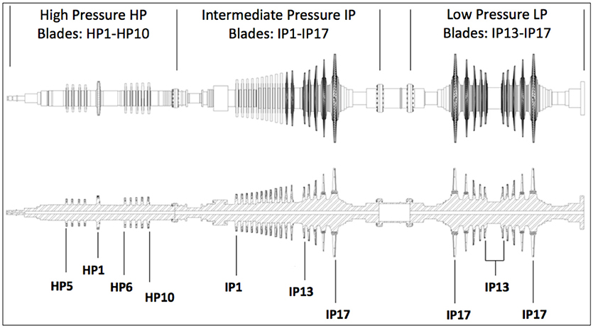
Figure 1. High, intermediate and low pressure turbines with numbered stages.

The organization of this work is set as follows. The theoretical formulation of the actual measure of fit of the updating methodology based on modal modes, modal frequencies and frequency response functions is briefly presented in section Formulation of Objective Function. Section Linear FE Model Updating Framework presents the implemented FE model updating methodology. Section Reverse Engineering Strategy presents the 3D digitization of the blades and the 2D designing of the three shafts of the individual sections of the complete turbine, as well as their combination leading to the final parametric CAD model. Next, the experimental modal identification procedure is described, in order to identify modal modes and frequencies of the actual structures of the intermediate pressure sections. The updating results of the parameterized intermediate pressure turbine is presented in section Finite Element Model Updating. Section Rotordynamic Analysis of the Simplified Equivalent Model of the Complete Steam Turbine presents a brief formulation and a rotordynamic analysis of the introduced simplified FE model based on Timoshenko beam and disk elements. Finally, some conclusions about the applicability and future work are summarized in section Conclusions.

Formulation of Objective Function

Modal Measure of Fit

We consider the data $D=\{{\widehat{\lambda }}_r,\underset{\_}{\widehat{{\phi }_r}}\in R^{N_{o,r}},r=1,\cdots ,m\}$ to be the squared of the measured modal frequencies, ${\widehat{\lambda }}_r={\widehat{\omega }}_r^2$ and the respective mode shapes $\underset{\_}{\widehat{{\phi }_r}}$ of the examined turbines, where N_o,r is the number of measured components for each r and m is the number of identified modes. Consider a parameterized linear FE model of the structures and let $\underset{\_}{\theta }\in R^{N_{\theta }}$ be a vector of free material model parameters to be tuned. The objective is to estimate the values of the parameter set θ so that the predicted modal frequencies and mode shapes $\{{\lambda }_r(\underset{\_}{\theta }),\underset{\_}{{\phi }_r}(\underset{\_}{\theta })\in R^{N_{0,r}},r=1,\cdots ,m\}$ at the corresponding N_0,r DOFs, diminishes discrepancies between modal frequencies identified in D. Thus, the modal frequency and mode shape residualsh are formulated as Mottershead et al. (2011); 2015a,b, Giagopoulos and Arailopoulos (2016), and Arailopoulos and Giagopoulos (2016):

${\epsilon }_{{\lambda }_r}^2(\underset{\_}{\theta })=\frac{{\left({\lambda }_r(\underset{\_}{\theta })-{\widehat{\lambda }}_r\right)}^2}{{\widehat{\lambda }}_r^2}\text{and }{\epsilon }_{\underset{\_}{{\varphi }_r}}^2(\underset{\_}{\theta })=\frac{{\Vert {\beta }_r(\underset{\_}{\theta })\underset{\_}{{\varphi }_r}(\underset{\_}{\theta })-\widehat{\underset{\_}{{\varphi }_r}}\Vert }^2}{{\Vert \widehat{\underset{\_}{{\varphi }_r}}\Vert }^2}(1)$

where ||Z||² = Z^TZ is the usual Euclidean norm, and ${\beta }_r(\underset{\_}{\theta })={\underset{\_}{\widehat{{\varphi }_r}}}^T\underset{\_}{{\varphi }_r}(\underset{\_}{\theta })/{\Vert \underset{\_}{{\varphi }_r}(\underset{\_}{\theta })\Vert }^2$ is a normalization constant that guaranties that the measured mode shape $\underset{\_}{\widehat{{\varphi }_r}}$ at the measured DOFs is closest to the model mode shape ${\beta }_r(\underset{\_}{\theta })\underset{\_}{{\varphi }_r}(\underset{\_}{\theta })$ predicted by the particular value of θ.

J₁(θ) and J₂(θ) are selected to represent the measure of fit between the measured and the model predicted frequencies and modes in the form:

$J_1(\underset{\_}{\theta })={\displaystyle \sum _{r=1}^m{\epsilon }_{{\lambda }_r}^2(\underset{\_}{\theta })}and{J}_2(\underset{\_}{\theta })={\displaystyle \sum _{r=1}^m{\epsilon }_{{\underset{\_}{\varphi }}_r}^2(\underset{\_}{\theta })}(2)$

Frequency Response Measure of Fit

A global shape correlation coefficient between experimentally identified and numerically predicted FRFs may be used (Grafe, 1995, 1999) for any measured frequency point λ_k as follows:

$\begin{array}{ll}{x}_s({\lambda }_k)=\frac{{\left|{\left\{H_X({\lambda }_k)\right\}}^H\left\{H_A({\lambda }_k)\right\}\right|}^2}{\left({\left\{H_X({\lambda }_k)\right\}}^H\left\{H_X({\lambda }_k)\right\}\right)\left({\left\{H_A({\lambda }_k)\right\}}^H\left\{H_A({\lambda }_k)\right\}\right)}& (3)\end{array}$

where {H_X(λ_k)} is the experimentally identified FRFs whereas as {H_A(λ_k)} are the numerically computed FRFs at matching excitation locations and response directions. As the MAC value, x_s(λ_k) assumes a value between zero and unity and indicates perfect correlation with x_s(λ_k) = 1. For x_s(λ_k) = 1, experimental and numerical data perfectly correlate contrary to the value of zero pertaining to no correlation at all. If only one measurement is utilized, {H_X(λ_k)} and {H_A(λ_k)} are reduced from column vectors to scalar and x_s = 1 across the full frequency spectrum for uncorrelated FRFs.

Thus, a supplementary amplitude correlation coefficient x_a(λ_k), for any measured frequency point λ_k is implemented quantifying the discrepancies in amplitude defined as:

$\begin{array}{ll}{x}_a({\lambda }_k)=\frac{2\left|{\left\{H_X({\lambda }_k)\right\}}^H\left\{H_A({\lambda }_k)\right\}\right|}{\left({\left\{H_X({\lambda }_k)\right\}}^H\left\{H_X({\lambda }_k)\right\}\right)+\left({\left\{H_A({\lambda }_k)\right\}}^H\left\{H_A({\lambda }_k)\right\}\right)}& (4)\end{array}$

defined to lie between zero and unity only if {H_A(λ_k)} = {H_X(λ_k)}.

J₃(θ) and J₄(θ) are selected to represent the measure of fit corresponding to the identified and predicted FRFs of the system:

$J_3(\underset{\_}{\theta })={\displaystyle \sum _{r=1}^m\left[1-x_s{({\widehat{\lambda }}_r,\underset{\_}{\theta })}^2\right]}\text{\hspace{0.17em}and\hspace{0.17em}}{J}_4(\underset{\_}{\theta })={\displaystyle \sum _{r=1}^m\left[1-x_a{({\widehat{\lambda }}_r,\underset{\_}{\theta })}^2\right]}(5)$

Objective Function

The overall measure of fit is formulated by a single objective function as follows:

$J(\underset{\_}{\theta };\underset{\_}{w})=w_1{J}_1(\underset{\_}{\theta })+w_2{J}_2(\underset{\_}{\theta })+w_3{J}_3(\underset{\_}{\theta })+w_4{J}_4(\underset{\_}{\theta })(6)$

using the weighting factors w_i ≥ 0, i = 1,2,3,4, with w₁ + w₂ + w₃ + w₄ = 1. The choice of weights scales each measure of fit according to the confidence in the experimental and FE predicted data, highly affecting the global minimum and the optimized solutions for the parameter set θ for given w are denoted by $\widehat{\theta }(w)$ (Christodoulou et al., 2008; Ntotsios and Papadimitriou, 2008; Papadimitriou et al., 2012; Giagopoulos et al., 2013).

Linear FE Model Updating Framework

As the objective function J(θ) is not an analytical expression, a stochastic black box search algorithm, namely the Covariance Matrix Adaptation Evolution Strategy (CMA-ES) (Hansen et al., 2003; Hansen, 2006, 2011) is implemented in this work as has been previously successfully applied for tuning linear and nonlinear FE models (Giagopoulos and Arailopoulos, 2017). The aim is to iteratively find the candidate solutions of the parameter set θ ∈ ${R}$ⁿ that produce the minimum J(θ), where the function values are sampled from a multivariate normal distribution in each iteration (Hansen, 2006, 2011).

CMA-ES avoids entrapment in local minima, reaching the global optimum of the sampled objective function. The algorithm is coupled to a commercial FE solver Dynamis (DTECH, 2013) surpassing the need of model reduction or sub-structuring techniques and taking advantage of the raw experimental measurements for increased accuracy. Thus, having the ability to compare modal modes and frequency response functions node by node and modal frequencies in a large frequency range overall fidelity of the updated FE models to the real structures is highly maintained. Moreover, due to the extremely large scale of the developed FE models and the numerous iterations needed to convergence a parallel computing scheme is applied in order to compensate for the computation time. Details on the formulation sequence of CMA-ES and the applied framework can be found in Giagopoulos and Arailopoulos (2017).

The minimum offsprings become parents in the next set of iterations and statistical values (mean and covariance matrix) are updated in a sequence of iterations with improved fitness values. The described framework runs in parallel in order to sample the prescribed population at once, in order to produce the total runs of each generation. Next, convergence criteria are checked. Introduced criteria include a given threshold of the objective function J(θ) = 0, being practically inapplicable and the difference of the best values of two consecutive sets of iterations ΔJ(θ) = 10⁻³.

Reverse Engineering Strategy

An integrated reverse engineering methodology is presented in total in this section on the steam turbine system currently operating at a thermal power plant of the Greek Public Power Corporation. The methodology combines modern techniques for geometry representation and development of the CAD and FE models, contemporary methods of modal identification and estimation of the dynamic characteristics of the physical structure from acceleration measurements and state-of-the-art model updating techniques, in order to produce a high fidelity FE model adequately simulating the steam turbine system.

The high, intermediate, and low pressure turbines are presented in Figures 2A–C respectively, under regular maintenance. The structure is made of steel with Young's modulus E = 210GPa, Poisson's ratio v = 0.3 and density ρ = 7850kg/m³ (Giagopoulos et al., 2017).

FIGURE 2

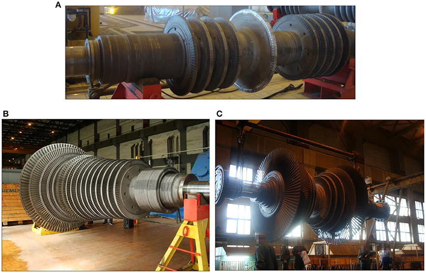
Figure 2. (A) High pressure turbine. (B) Intermediate pressure turbine. (C) Low pressure turbine.

Digitization and CAD Model of the Steam Turbine

At first, using two types of 3D scanner devices, i.e., a structured light and a laser scanner, the digital shape of each blade was reconstructed. The collection of the raw data and the consecutive processing to the development of the final CAD model are completed in four basic steps as demonstrated in Figure 3. First, the geometry of each blade was captured, so as to collect a raw stereo-lithography (STL) file. Due to various flaws and imperfections of the initial design such as holes, humps, coarse and non-continuous surfaces, the second step was to use compatible software in order to design the final STL file of the captured geometry, before designing the CAD model (Béchet et al., 2002; Bianconi, 2002; Rypl and Bittnar, 2006). The next step was the preparation of the consecutive foil sections that represent each blade. After aligning the scanned geometry, automated curves were created by section along the length of the main body of the blade at varying increments, depending on its length and complexity as well as on designing needs. These curves were parallel to each other as well as to base of the blades. Last, step was to select the most representable curves of each blade and use them to reconstruct the CAD models.

FIGURE 3

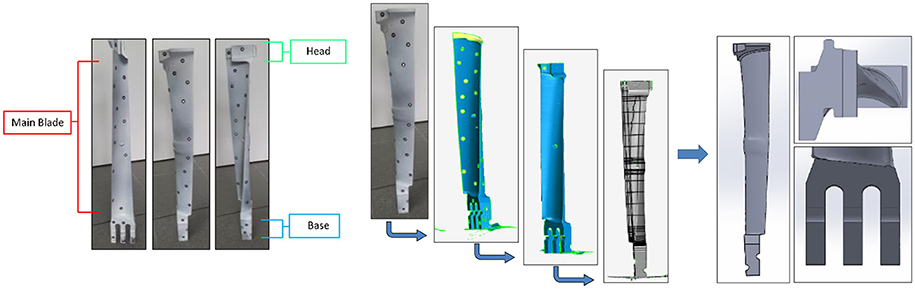
Figure 3. Digitization and final 3D CAD model of a single blade at stage IP 15 of the intermediate pressure turbine.

On top of designing the main body of the blades, bases, and heads were designed from scratch under meticulous measurements. Four blades were cover by heads that were designed separately and placed on top of the main body using vertical curves, in order to succeed the finest positioning. Additionally, all bases of the blades were designed separately taking into consideration their slight curvature, in order to tangently fit around the rotor shaft. Finally, the top of each base was designed flat in order to fit perfectly with the main body of the blade.

In order to design the rotor shafts of the steam turbine, the technical drawings were used. The blueprints were hardcopies of the high, intermediate, and low pressure turbines in manageable scale used in order to produce the 2D axisymmetric design of the shafts.

Combining the complete CAD models of the blades with the three rotor shafts, the final CAD model of the complete steam turbine was created. The following Figures 4A–C present the rotor shafts and the complete 3D CAD models of the high, intermediate and low pressure turbines respectively. Furthermore, the final 3D CAD model of the complete steam turbine is presented in Figure 4D.

FIGURE 4

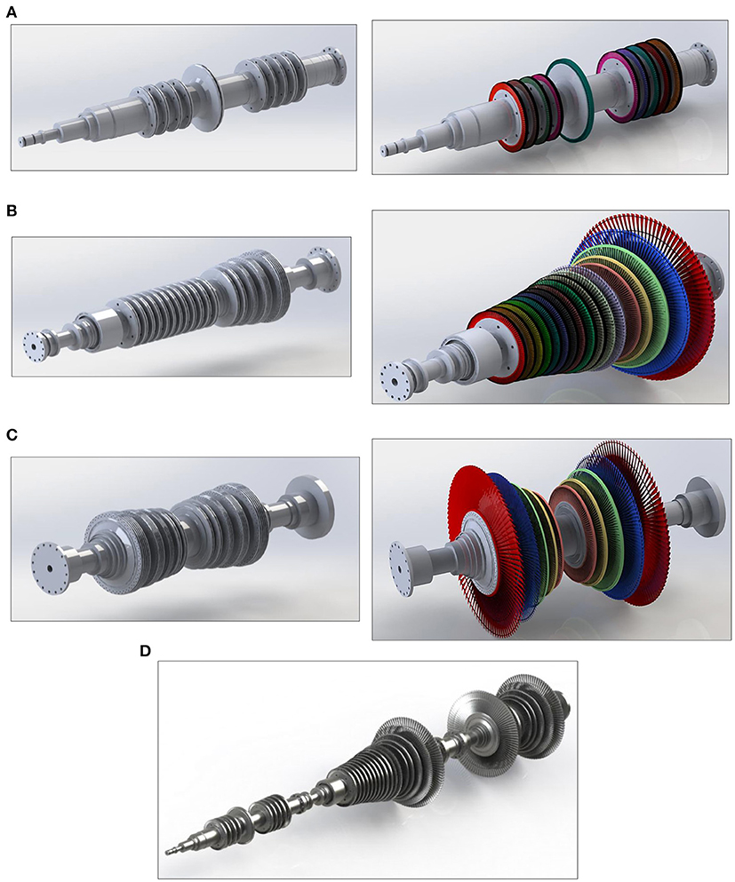
Figure 4. (A) Rotor shaft and complete 3D CAD assembly of the high pressure turbine. (B) Rotor shaft and complete 3D CAD assembly of the intermediate pressure turbine. (C) Rotor shaft and complete 3D CAD assembly of the low pressure turbine. (D) Final 3D CAD of the complete steam turbine.

FE Models of Steam Turbine Rotor

The geometry of the turbine sections is discretized by solid elements (tetrahedral). Due to the complex geometry of the structure, the total number of degrees of freedom of the high, intermediate, and low pressure sections were about 10,000,000, 20,000,000, and 19,500,000 respectively, whereas the resulting complete rotor model was about 55,000,000 degrees of freedom, including the connection parts between the sections. The detailed FE models of the high, intermediate and low pressure turbines are presented in Figure 5A respectively and Figure 5B depicts the final finite element model of the complete steam turbine. FE pre-processor software and FE analysis software were used in order to develop and analyze the FE model (DTECH, 2013; BETA CAE Systems, 2018). Indicative mode shapes of the three sections in a free-free state and the complete model with typical supports are presented in Figure 6.

FIGURE 5

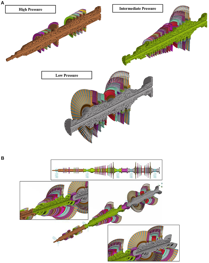
Figure 5. (A) Detailed FE models of the high, intermediate, and low pressure turbines. (B) Detailed FE models of the complete steam turbine.

FIGURE 6

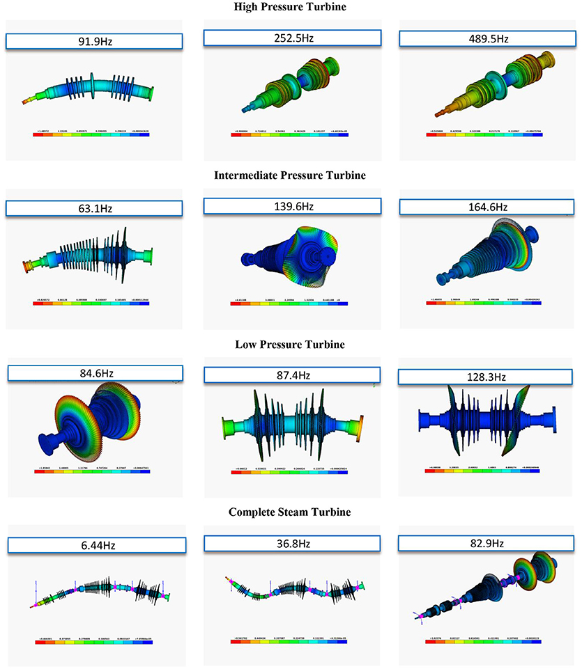
Figure 6. Indicative eigenmodes of the high, intermediate and low pressure sections and the complete steam turbine predicted by the nominal FEM.

Experimental Modal Analysis

In this section the dynamic characteristics of the complete steam turbine are identified in order to compute the measure of fit between numerical FE model and actual structure. In order to quantify the dynamic characteristics of the complete steam turbine, an experimental modal analysis of the three turbine sections was performed. Due to large size of the results, it is selected to present the results only for the intermediate pressure rotor.

An industrial size crane was used to mount each turbine separately, simulating a support-free state for the experimental procedure. Impulsive loading was imposed at various locations and directions on the structure in order to estimate the elements of the FRF matrix—Equation (7) (Ewins, 1984; Mohanty and Rixen, 2005; Giagopoulos and Natsiavas, 2007, 2015; Spottswood and Allemang, 2007).

$\begin{array}{ll}\left[\begin{array}{c}{ü}_1\\ {\ddot{v}}_1\\ {ẅ}_1\\ \cdots \\ {ẅ}_n\end{array}\right]={\left[\begin{array}{ccc}H{u}_1{u}_1& \cdots & H{u}_1{w}_n\\ H{v}_1{u}_1& \cdots & H{v}_1{w}_n\\ H{w}_1{u}_1& \cdots & H{w}_1{w}_n\\ ⋮& \ddots & ⋮\\ H{w}_n{u}_1& \cdots & H{w}_n{w}_n\end{array}\right]}_{3n\times 3n}{\left[\begin{array}{c}F{u}_1\\ ⋮\\ F{w}_n\end{array}\right]}_{{}_{3n\times 3n}}& (7)\end{array}$

The frequency range of 0–2048 Hz was obtained during measurements, including the numerical frequency range of interest, i.e., 0–200 Hz including the first ten modal frequencies. A schematic illustration of the measurement geometry for the modal analysis of the intermediate pressure rotor, with the real experimental set up of this test is presented in Figure 7. For instance, Figure 8 presents the magnitude of representative elements of the FRF matrix.

FIGURE 7

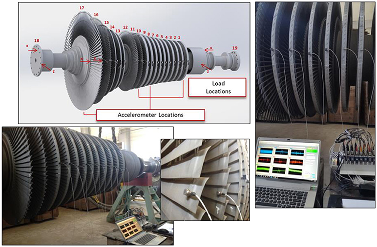
Figure 7. Experimental set-up of the intermediate pressure turbine.

FIGURE 8

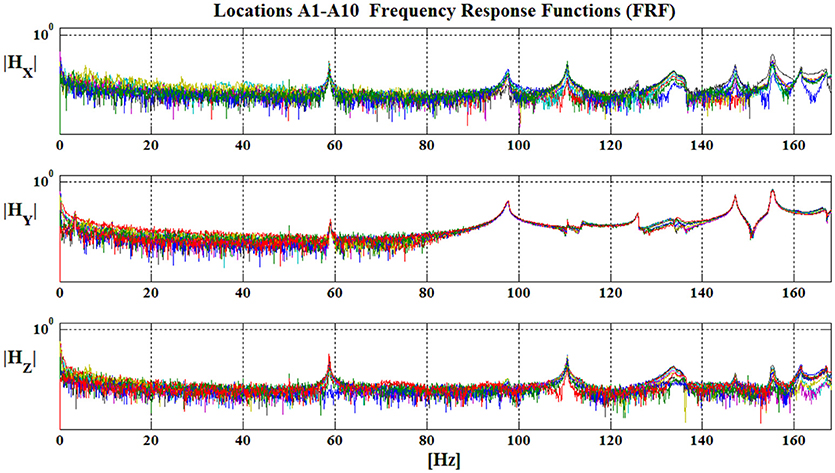
Figure 8. Typical elements of the experimental FRF matrix for the intermediate pressure rotor.

The Rational Fraction Polynomial Method (RFPM) (Richardson and Formenti, 1985; Friswell and Penny, 1990; Ntotsios and Papadimitriou, 2008) was used in order to estimate the experimental natural frequencies and the damping ratios of the intermediate pressure turbine, based on the measured FR functions.

Indicatively, two typical elements of the experimentally measured FRF matrix of the intermediate pressure turbines are compared to the estimated RFPM contours as presented in Figure 9. The same figure also presents the experimentally measured and analytically estimated time histories. The FR functions corresponding to accelerometers A3 and A7 of the intermediate pressure section at Y local component are presented in Figure 9. The red line corresponds to the experimentally measured FRF and time history compared to the dashed blue line corresponding to the estimated contour filtered with Welch's (1967) method. Additionally, all experimentally modal mode shapes are identified, in order to be used in the formulation of the measure of fit passed to the optimization algorithm.

FIGURE 9

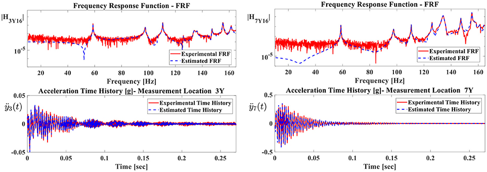
Figure 9. Comparison of FRFs and time histories of accelerations corresponding to frequency response functions |H_3Y16| and |H_7Y16| of accelerometers A3 and A7 at local direction Y.

Table 1 summarizes the experimental modal analysis results for the intermediate pressure turbine. The values of the lowest natural frequencies ω_rE, are presented in the second column of Table 1 whereas the fifth column list the corresponding damping ratios. The values of the natural frequencies predicted from the numerical model ω_rNFE using nominal material parameters using lumped mass matrix implemented in solver Dynamis (DTECH, 2013), are listed in the third column whereas a comparison is presented in the fourth column. The underestimation of the predicted natural frequencies of the nominal FE model, is attributed to the way Dynamis handles mass matrix. In spite of the fairly insignificant discrepancies between the nominal FE model and the experimental data, a subsequent FE model updating process is necessary to diminish these errors.

TABLE 1

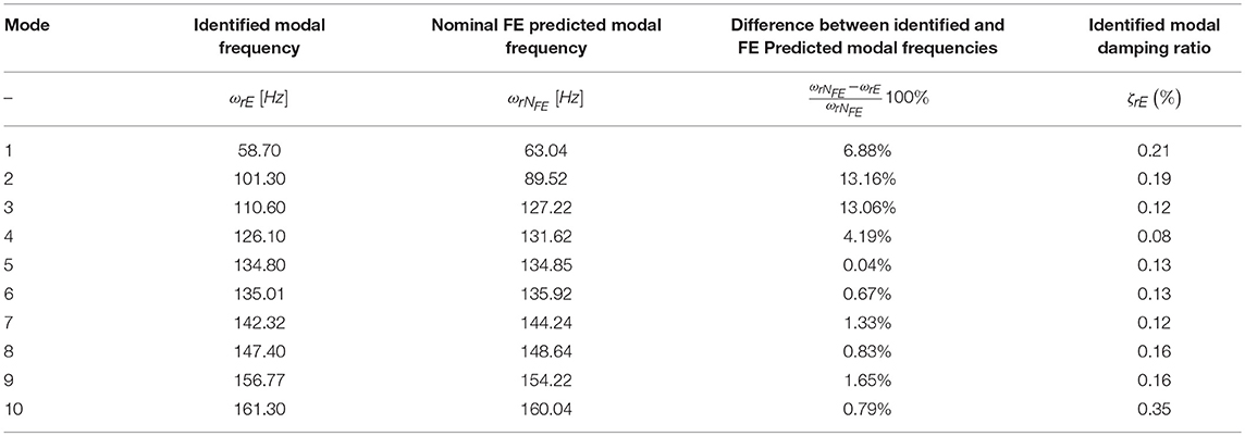
Table 1. Identified and nominal FEM predicted modal frequencies and modal damping ratios of the intermediate pressure turbine.

The accuracy of the experimental measurements highly depends on the quality of the experimental devices and the abilities of the users. Inaccurate measurement data could be produce by a defective apparatus or user mishandling. The reliability of the collected data during the experimental procedures was checked, from the small variation of the data. Such an examination is imperative as the experimental results highly affect the accuracy of the overall technique.

Finite Element Model Updating

Parameterization of FE Models

In this section, the parameterization of the finite element model of the intermediate section is introduced in order to apply the updating methodology. This model consists of about 23 million degrees of freedom. The parameterized model consisting of 44 parts which is shown in Figure 10. At each of these parts are used as design variables the Young's modulus and the density. Thus, the final number of the design parameters are eighty-eight (88) variables. The first parts describe the rotor shafts whereas each stage is modeled with two or three parts. Two parts are used to model the blades and their circumferential ring at small diameter stages, whereas three parts are used to model eight large diameter stages of the intermediate pressure assigning two parts for the blades and one for the circumferential ring. Although both the rotor shaft and the turbine blades have been built from a single material, steel, the mechanical treatment that all parts undertake in order to take their final form and shape as well as their assembly may change the overall stiffness of the structure related to an FE model where assumption are made beforehand. Specifically, molding of the steel during industrial manufacturing of the turbine parts may result in slight variation of the modulus of elasticity and density of the actual used material. Additionally, remaining stresses may develop that increase stiffness. Furthermore, the tight assembly of the blades on the rotor shaft and between each other, result in additional remaining stresses that could not be modeled in the FEM and could only be handled by tuning the material propertied. In this direction the parameter space for each design variable, was selected in the range of ± 10% of the nominal values, introducting the upper and lower constraints of material properties, in order to maintain realistic values and keep their physical meaning.

FIGURE 10

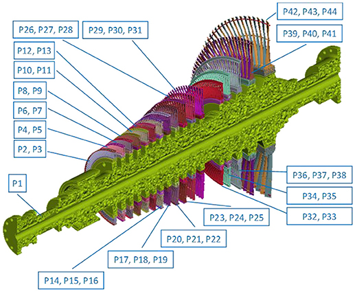
Figure 10. Parts of the parameterized FE models of the intermediate pressure turbines.

The finite element model is updated using the ten identified modal frequencies and mode shapes shown in Table 1. Components at all 17 sensor locations are used in identification of the mode shapes of the structure. Moreover, the total weight of the FE model is defined as a global behavioral design constraint, apart from the box constraints of the design variables in the optimization process. This global behavioral constraint was implemented in order to reject and resample the material parameters chosen from the design space of the boxed (lower and upper bound) constraints, that produce a total weight of the FE model that varies significantly from the actual weight of the structure.

Model Update Results and Verification

The CMA-ES framework introduced in previous work (Giagopoulos and Arailopoulos, 2017) is applied to update the developed FE models. During FE model analyses, no model reduction or sub-structuring methodologies were applied in order to increase accuracy with regard to the real structures. Furthermore, the large number of degrees of freedom of each FE model in conjunction with the numerous amount of sampling needed by CMA-ES for convergence, required prohibitive time, at high computational cost. Thus, a parallelized scheme of the applied algorithm, coupling FE solver Dynamis (DTECH, 2013) to CMA-ES was implemented, as has been previously demonstrated in Giagopoulos and Arailopoulos (2017), in order to counterbalance computational cost effectiveness and render possible and applicable such an optimization methodology at an extremely large scale FE model. Indicatively, the optimization process was running for ~15 days for the intermediate pressure turbine. The computer that was used, hosts two (2) Intel^® Xeon^® Processors E5-2630 v3 (20M Cache, 2.40 GHz) with 8-cores and 16-threads, resulting in a total number of thirty-two (32) logical (virtual) cores and 64 GB of RAM, on Linux Ubuntu 16.04 Operating System.

Table 2 presents the design vector of the optimized material properties of indicative parts of the intermediate pressure turbine. Part P1 corresponds to the rotor shaft, and the optimized parameters lie close to the nominal parameter values of steel, as it is the only part of the turbine that is almost intact and unaffected by its long time operation. Parts P3, P9, P27, P30, P33, P35, and P43 correspond to the optimized material properties that showed maximum deviation from the nominal values. All parts are related to blades. Blades are the most vulnerable parts of the turbine that corrode during operation and need regular maintenance. Additionally, all blades are tightly fixed with steel rods producing remaining stresses that increase stiffness.

TABLE 2

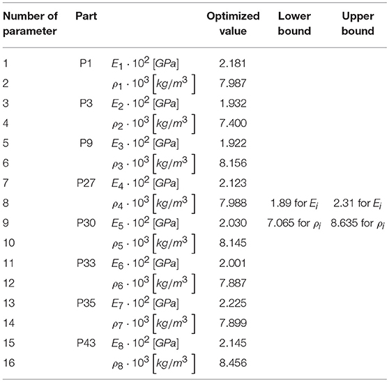
Table 2. Optimized parameter values of material properties for rotor shaft and indicative blades of the intermediate pressure turbine.

Convergence has been achived with respect to the objective function using the convergence critterion as defind in section Linear FE Model Updating Framework being the difference of the best values of two consecutive sets of iterations ΔJ(θ) = 10⁻³. In order to equally consider the contribution of the four residuals, equal weighting factors were chosen. Different weighting factors would account for increased reliability of the formulation of one of the four residuals, arisen from experience or experimental confidence.

Figure 11 presents the history of convergence, where the objective function value is presented against number of iterations where we can see the fast convergence rate and Table 3 presents the updated modal frequencies along a comparison between the identified (ω_rE) and optimized FE predicted modal frequencies (ω_rOFE). A slight difference between optimal and experimental modal frequencies is inevitable due to various uncontrolled uncertainties.

FIGURE 11

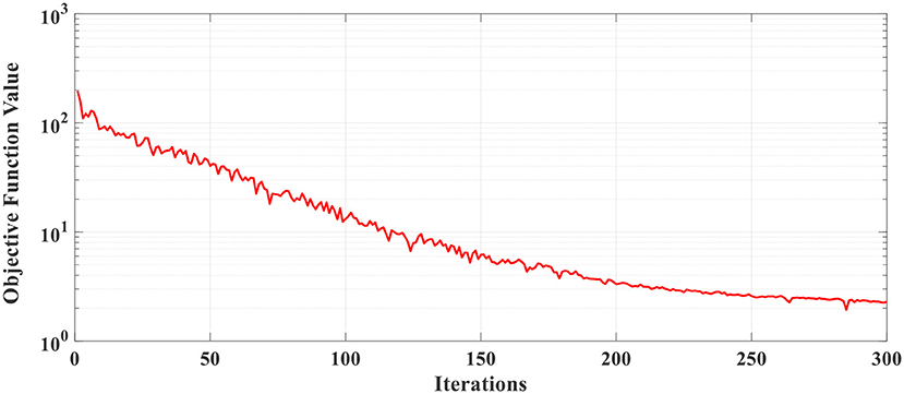
Figure 11. Objective function values diagram of intermediate pressure turbine.

TABLE 3

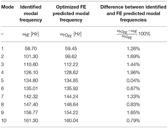
Table 3. Identified and optimized FE predicted modal frequencies of the intermediate pressure turbine.

Rotordynamic Analysis of the Simplified Equivalent Model of the Complete Steam Turbine

The analyses presented refer to the system in free oscillation, having omitted the rotation speed of the rotor and having no knowledge of the effect of gyroscopic and shear phenomena due to rotation. The large scale of the developed finite element model renders the rotordynamic analysis from extremely computationally expensive to impossible. Thus, a simplified model of the turbine, which takes into account the gyroscopic phenomena occurring during the rotation of the turbine, was introduced in Matlab (Mathworks, 2016) using the freeware scripts of rotor software (Friswell et al., 2010b) developed for analyzing the dynamics of rotating machines (Friswell et al., 2010a). The simplified model was tested for the accuracy of its results with the developed complete finite element model by modal analysis in idle position. Based on the full-scale steam turbine, the simplified FE model consists of 73 Timoshenko beam elements simulating the shaft and 37 disk elements simulating the stages of the blade elements of the turbine. The total number of nodes was 74 and at 5 nodes isotropic bearing elements were placed in all directions that refer to the bearing point of the rotor. Figure 12 illustrates the simplified model of the steam turbine, where cyan color is the shaft elements, green dots refer to the nodes, yellow color represents the blades of each stage and red triangles show the bearing of the rotor.

FIGURE 12

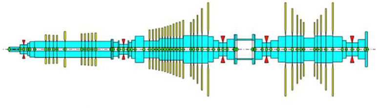
Figure 12. Schematic illustration of simplified FE model of the complete steam turbine.

The updated material parameters of the full model of the turbine were used, for the axis properties. The only difference is in the density of the disks. As each stage consists of a large number of blades that obviously have a gap between them, they cannot be modeled as solid disc. Thus, the density of the disk was adjusted according to the actual volume and the actual mass of the stage from the full-scale FE model. Firstly, frequencies of the simplified model at zero rotational speed (idle) were compared to those of the complete FE model as presented in Table 4. Specifically, the second and third columns present the frequencies of the simplified and full-scale FE models, whereas the last column presents the deviation between them.

TABLE 4

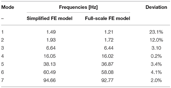
Table 4. Comparison between modal frequencies of the simplified FE model at idle state and the full-scale FE model.

Indicatively the 2nd, 4, and 5th modes of the full-scale and the simplified for zero rotation speed, FE models are presented in Figure 13. We notice that the modes are very similar to both models. Coloring the results of the simplified and full-scale model based on displacements, helps us understand the movement of the body at each mode. Thus, the coloration of the simplified model in red line correspond to the shaft and the blue lines to the displacements of the internal nodes, whereas the coloration of the full-scale FE model is depicted on the colored legend.

FIGURE 13

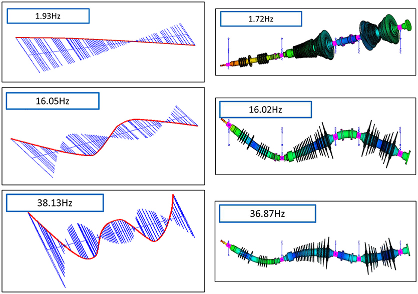
Figure 13. 2nd, 4, and 5th eigenmodes of the simplified FE model at idle state at 1.93, 16.05, and 38.13 Hz and equivalent eigenmodes of the full-scale FE model at 1.72, 16.02, and 36.87 Hz.

Moreover, at 50 Hz, which is the electric current frequency, the turbine will rotate at 3,000 rpm. Table 5 summarizes the 30 first rotational frequencies of the simplified model at 3,000 rpm rotational speed. Indicative modes are presented in Figure 14. The simplified FE model could be further updated in regard to the bearings for increased accuracy and fidelity to the real steam turbine structure at working state. Specifically, experimental vibration measurements could be collected at all bearing points under real working conditions, in order to update the stiffness and damping parameters at all supporting directions during rotation of the steam turbine at operational spin speed. The thick black line represents the rotor axis while the vertical circular lines represent the orbits of the nodes in a period of rotation.

TABLE 5

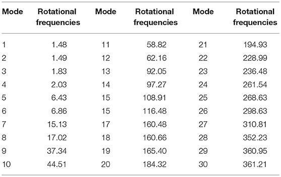
Table 5. Rotational eigenfrequencies of the simplified model at 3,000 rpm rotational speed.

FIGURE 14

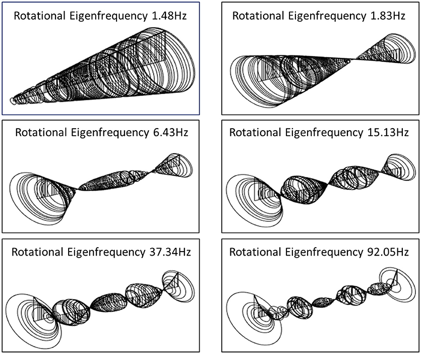
Figure 14. Indicative rotational eigenmodes 1, 3, 5, 7, 9, and 13 corresponding to 1.48, 1.83, 6.43, 15.13, 37.34, and 92.05 Hz of the simplified FE model at 3,000 rpm rotational speed.

Finally, Figure 15 presents the Campell diagram (Campbell, 1924; Meher-Homji and Prisell, 2005) of turbine's response spectrum as a function of spin speed, at a range of 0–4,500 rpm which represents the variation of the rotational frequencies as the rotation speed changes.

FIGURE 15

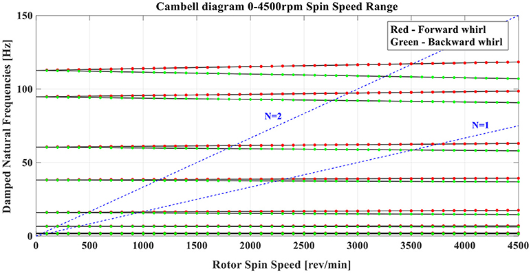
Figure 15. Cambell diagram at 0–4.500 rpm spin speed range.

Conclusions

An integrated reverse engineering methodology is presented in this work on a large-scale steam turbine rotor, taking into account issues related to the development of the CAD and FE model, experimental modal analysis procedures and the application of robust and effective computational finite element model updating techniques. Numerical and experimental methodologies were implemented in order to identify the model parameters and develop a high fidelity finite element model of the examined structure. An extensible framework of CMA Evolution Strategy for complex and computationally demanding physical models is implemented in order to finely tune material parameters, such as modulus of elasticity and density, in order to best match experimental and numerical data. Moreover, a simplified FE model based on the updated full large-scale FE model of the steam turbine is introduced, in order to get deep insight of the rotordynamic behavior and gyroscopic effects of the examined rotor. Accumulated knowledge of the dynamic behavior of the steam turbine system, could be later implemented in order to evaluate stability or instability states, fatigue growth in the turbine blades, changes in the damping of the bearing system and perform necessary scheduled optimal and cost-effective maintenance strategies. Additionally, upon a series of scheduled experimental data collection, a permanent output-only vibration SHM system could be installed and even a proper dynamic balancing could be investigated and designed.

Author Contributions

DG was involved in the development of the computational framework, finite element models and experimental modal analysis, AA with the development of the computational framework and the finite element model updating, while IZ and EP with the scanning of the surfaces and the development of three-dimensional geometry.

Conflict of Interest Statement

The authors declare that the research was conducted in the absence of any commercial or financial relationships that could be construed as a potential conflict of interest.

The reviewer, ARC, and handling editor declared their shared affiliation.

References

Abella, R. J., Daschbach, J. M., and McNichols, R. J. (1994). Reverse engineering industrial applications. Comp. Indus. Eng. 26, 381–385. doi: 10.1016/0360-8352(94)90071-X

CrossRef Full Text | Google Scholar

Arailopoulos, A., and Giagopoulos, D. (2016). “Finite element model updating techniques of complex assemblies with linear and nonlinear components,” in 34th IMAC, A Conference and Exposition on Structural Dynamics, 2016 (Orlando, FL: Springer New York LLC).

Google Scholar

Bavastri, C. A., Ferreira, E. M. D. S., Espíndola, J. J. D., and Lopes, E. M. D. O. (2008). Modeling of dynamic rotors with flexible bearings due to the use of viscoelastic materials. J. Br. Soc. Mech. Sci. Eng. 30, 22–29. doi: 10.1590/S1678-58782008000100004

CrossRef Full Text | Google Scholar

Béchet, E., Cuilliere, J. C., and Trochu, F. (2002). Generation of a finite element MESH from stereolithography (STL) files. Comput. Aided Des. 34, 1–17. doi: 10.1016/S0010-4485(00)00146-9

CrossRef Full Text | Google Scholar

Beck, J. L. (2011). “Bayesian updating, model class selection and robust stochastic predictions of structural response,” in Proceedings of the 8th International Conference on Structural Dynamics, EURODYN 2011 (Leuven).

Google Scholar

Beck, J. L., and Katafygiotis, L. S. (1998). Updating models and their uncertainties. I: Bayesian statistical framework. J. Eng. Mech. 124, 455–461.

Google Scholar

BETA CAE Systems, S.A. (2018). ANSA and META-Post. Thessaloniki: BETA CAE Systems. S.A.

Bianconi, F. (2002). Bridging the gap between CAD and CAE using STL files. Int. J. CAD CAM 2, 55–67.

Google Scholar

Booysen, C., Heyns, P. S., Hindley, M. P., and Scheepers, R. (2015). Fatigue life assessment of a low pressure steam turbine blade during transient resonant conditions using a probabilistic approach. Int. J. Fatig. 73, 17–26. doi: 10.1016/j.ijfatigue.2014.11.007

CrossRef Full Text | Google Scholar

Campbell, W. (1924). Protection of Steam Turbine Disk Wheels from Axial Vibration. Schenectady, NY: General electric Co.

Christodoulou, K., Ntotsios, E., Papadimitriou, C., and Panetsos, P. (2008). Structural model updating and prediction variability using Pareto optimal models. Comp. Methods Appl. Mech. Eng. 198, 138–149. doi: 10.1016/j.cma.2008.04.010

CrossRef Full Text | Google Scholar

Dagli, C. H., and Idowu, M. A. (2015). “Instantaneous modelling and reverse engineering of data-consistent prime models in seconds,” in Procedia Computer Science Complex Adaptive Systems (San Jose, CA), 373–380.

DTECH (2013). DYNAMIS 3.1.1. Thessaloniki: DTECH.

Ewins, D. J. (1984). Modal Testing: Theory and Practice. Somerset: Research Studies Press.

Eykhoff, P. (1974). System Identification Parameter and State Estimation. London, UK: John Wiley & Sons, Inc.

Friswell, M. I., and Penny, J. E. T. (1990). Updating model parameters from frequency domain data via reduced order models. Mech. Syst. Signal Process. 4, 377–391. doi: 10.1016/0888-3270(90)90064-R

CrossRef Full Text | Google Scholar

Friswell, M. I., Penny, J. E. T., Garvey, S. D., and Lees, A. W. (2010a). Dynamics of Rotating Machines. Cambridge Aerospace Series. Cambridge, CA: Cambridge University Press.

Google Scholar

Friswell, M. I., Penny, J. E. T., Garvey, S. D., and Lees, A. W. (2010b). Rotordynamics Software Manual, in Dynamics of Rotating Machines. Cambridge: Cambridge University.

Google Scholar

Giagopoulos, D., and Arailopoulos, A. (2015a). “Finite element model updating of geometrically complex structure through measurement of its dynamic response,” in 1st ECCOMAS Thematic Conference on Uncertainty Quantification in Computational Sciences and Engineering, UNCECOMP 2015 (Crete Island: National Technical University of Athens).

Giagopoulos, D., and Arailopoulos, A. (2015b). “Parameter identification of complex structures using finite element model updating techniques,” in ASME 2015 International Design Engineering Technical Conferences and Computers and Information in Engineering Conference, IDETC/CIE 2015 (Boston, MA: American Society of Mechanical Engineers (ASME)).

Google Scholar

Giagopoulos, D., and Arailopoulos, A. (2016). “Parameter estimation of nonlinear large scale systems through stochastic methods and measurement of its dynamic response,” in 7th European Congress on Computational Methods in Applied Sciences and Engineering, ECCOMAS Congress 2016 (Crete Island: National Technical University of Athens).

Google Scholar

Giagopoulos, D., and Arailopoulos, A. (2017). Computational framework for model updating of large scale linear and nonlinear finite element models using state of the art evolution strategy. Comp. Struct. 192, 210–232. doi: 10.1016/j.compstruc.2017.07.004

CrossRef Full Text | Google Scholar

Giagopoulos, D., Arailopoulos, A., Zacharakis, I., and Pipili, E. (2017). “Finite element model developed and modal analysis of large scale steam turbine rotor: quantification of uncertainties and model updating,” in 2nd ECCOMAS Thematic Conference on Uncertainty Quantification in Computational Sciences and Engineering (UNCECOMP) Rhodes Island: ECCOMAS.

Google Scholar

Giagopoulos, D., and Natsiavas, S. (2007). Hybrid (numerical-experimental) modeling of complex structures with linear and nonlinear components. Nonlinear Dynam. 47, 193–217. doi: 10.1007/s11071-006-9067-3

CrossRef Full Text | Google Scholar

Giagopoulos, D., and Natsiavas, S. (2015). Dynamic response and identification of critical points in the superstructure of a vehicle using a combination of numerical and experimental methods. Exp. Mech. 55, 529–542. doi: 10.1007/s11340-014-9966-z

CrossRef Full Text | Google Scholar

Giagopoulos, D., Papadioti, D.-C., Papadimitriou, C., and Natsiavas, S. (2013). “Bayesian uncertainty quantification and propagation in nonlinear structural dynamics,” in Topics in Model Validation and Uncertainty Quantification, Volume 5: Proceedings of the 31st IMAC, A Conference on Structural Dynamics, 2013, eds T. Simmermacher, S. Cogan, B. Moaveni, and C. Papadimitriou (New York, NY: Springer), 33–41.

Google Scholar

Grafe, H. (1995). Review of Frequency Response Function Updating Methods. BRITE-URANUS BRE2-CT94-0946.

Grafe, H. (1999). Model Updating of Large Structural Dynamics Models Using Measured Response Function. London: Department of Mechanical Engineering, Imperial College.

Google Scholar

Hadjidoukas, P. E., Angelikopoulos, P., Papadimitriou, C., and Koumoutsakos, P. (2015). Π4U: a high performance computing framework for Bayesian uncertainty quantification of complex models. J. Comput. Phys. 284, 1–21. doi: 10.1016/j.jcp.2014.12.006

CrossRef Full Text | Google Scholar

Hadjidoukas, P. E., Lappas, E., and Dimakopoulos, V. V. (2012). “A runtime library for platform-independent task parallelism,” in 2012 20th Euromicro International Conference on Parallel, Distributed and Network-based Processing. (Garching).

Google Scholar

Hansen, N. (2006). The CMA evolution strategy a comparing review. Towards New Evol. Comput. 192, 75–102. doi: 10.1007/3-540-32494-1_4

CrossRef Full Text | Google Scholar

Hansen, N. (2011). The CMA Evolution Strategy: A Tutorial. Research centre Saclay –Île-de-France Universite Paris-Saclay, LRI.

Hansen, N., Müller, S. D., and Koumoutsakos, P. (2003). Reducing the time complexity of the derandomized evolution strategy with covariance matrix adaptation (CMA-ES). Evol. Comput. 11, 1–18. doi: 10.1162/106365603321828970

PubMed Abstract | CrossRef Full Text | Google Scholar

Mathworks (2016). MATLAB, Natick, MA: Mathworks Inc.

Meher-Homji, C. B., and Prisell, E. (2005). Dr. Max Bentele—pioneer of the jet age. J. Eng. Gas Turb. Power 127, 231–239. doi: 10.1115/1.1807412

CrossRef Full Text | Google Scholar

Mohanty, P., and Rixen, D. J. (2005). Identifying mode shapes and modal frequencies by operational modal analysis in the presence of harmonic excitation. Exp. Mech. 45, 213–220. doi: 10.1007/BF02427944

CrossRef Full Text | Google Scholar

Mottershead, J. E., Link, M., and Friswell, M. I. (2011). The sensitivity method in finite element model updating: a tutorial. Mech. Syst. Signal Process. 25, 2275–2296. doi: 10.1016/j.ymssp.2010.10.012

CrossRef Full Text | Google Scholar

Ntotsios, E., and Papadimitriou, C. (2008). “Multi-objective optimization algorithms for finite element model updating,” in International Con- ference on Noise and Vibration Engineering (ISMA2008). Leuven: Katholieke Universiteit Leuven, 66–80.

Google Scholar

Ouamer-Ali, M.-I., Laroche, F., Bernard, A., and Remy, S. (2014). “Toward a methodological knowledge based Approach for partial automation of reverse engineering,” in 24th CIRP Design Conference (Elsevier), 270–275. doi: 10.1016/j.procir.2014.03.190

CrossRef Full Text | Google Scholar

Papadimitriou, C., Ntotsios, E., Giagopoulos, D., and Natsiavas, S. (2012). Variability of updated finite element models and their predictions consistent with vibration measurements. Struct. Control Health Monit. 19, 630–654. doi: 10.1002/stc.453

CrossRef Full Text | Google Scholar

Plesiutschnig, E., Fritzl, P., Enzinger, N., and Sommitsch, C. (2016). Fracture analysis of a low pressure steam turbine blade. Case Stud. Eng. Fail. Anal. 5–6, 39–50. doi: 10.1016/j.csefa.2016.02.001

CrossRef Full Text | Google Scholar

Richardson, M. H., and Formenti, D. L. (1985). “Global curve fitting of frequency response measurements using the rational fraction polynomial method,” in Third IMAC Conference (Orlando, FL).

Google Scholar

Rypl, D., and Bittnar, Z. (2006). Generation of computational surface meshes of STL models. J. Comput. Appl. Math. 192, 148–151. doi: 10.1016/j.cam.2005.04.054

CrossRef Full Text | Google Scholar

Spottswood, S. M., and Allemang, R. J. (2007). On the investigation of some parameter identification and experimental modal filtering issues for nonlinear reduced order models. Exp. Mech. 47, 511–521. doi: 10.1007/s11340-007-9047-7

CrossRef Full Text | Google Scholar

Várudy, T., Martin, R. R., Cox, J., Várady, T., Martin, R. R., and Cox, J. (1997). Reverse engineering of geometric modelsreverse engineering of geometric models—an introduction. Comput. Aided Des. 29, 255–268. doi: 10.1016/S0010-4485(96)00054-1

CrossRef Full Text | Google Scholar

Wang, J., Gu, D., Yu, Z., Tan, C., and Zhou, L. (2012). A framework for 3D model reconstruction in reverse engineering. Comp. Ind. Eng. 63, 1189–1200. doi: 10.1016/j.cie.2012.07.009

CrossRef Full Text | Google Scholar

Welch, P. (1967). The use of fast Fourier transform for the estimation of power spectra: a method based on time averaging over short, modified periodograms. IEEE Trans. Audio Electroacoust. 15, 70–73. doi: 10.1109/TAU.1967.1161901

CrossRef Full Text | Google Scholar