Critical Ground Motion for Resilient Building Design Considering Uncertainty of Fault Rupture Slip

Introduction

Many peculiar earthquake ground motions have been observed in the world, e.g., Mexico (1985), Northridge (1994), Kobe (1995), Chi-chi (1999), Tohoku (2011), Kumamoto (2016). To model these ground motions from their occurrence mechanisms, several models have been proposed. The whole process of ground motion generation consists of (i) the fault rupture process, (ii) the wave propagation from fault to the earthquake bedrock, (iii) the site amplification. These models can be classified generally into the theoretical approach, the numerical analysis approach, the semi-empirical approach and the hybrid approach. In the theoretical approach and the numerical analysis approach, the wavenumber integration method and the finite difference method are the representatives and are suitable for the generation of directivity pulses and surface waves with the predominant period longer than 1–2 s (Bouchon, 1981; Hisada and Bielak, 2003; Yoshimura et al., 2003; Nickman et al., 2013). On the other hand, the semi-empirical approach is suitable for the generation of random ground motions with the predominant period shorter than 1–2 s and can generate a large ground motion in terms of small-size ground motions using the scaling law of fault parameters. The empirical Green's function (Wennerberg, 1990) and the stochastic Green's function (Hisada, 2008) are often used in the semi-empirical approach. The hybrid approach is the method which combines the random ground motions of shorter predominant period with the waves of longer predominant period by using a matching filter.

Although most of the previous approaches of ground motion generation were aimed at generating ground motions for a fixed set of parameters, several parameters should be treated as uncertain numbers (aleatory or epistemic) to make the approach more reliable (Abrahamson et al., 1998; Lawrence Livermore National Laboratory, 2002; Morikawa et al., 2008; Cotton et al., 2013).

As for researches on the effect of uncertainty of parameters on response variability, Taniguchi and Takewaki (2015) derived the bound of earthquake input energy to building structures by considering shallow and deep ground uncertainties and soil-structure interaction. Okada et al. (2016) proposed a new interval analysis technique for a soil-pile-structure interaction model by taking into account the uncertainty in soil properties. Makita et al. (2018) considered a base-isolation, building-connection hybrid structural system (Murase et al., 2013, 2014; Kasagi et al., 2016; Fukumoto and Takewaki, 2017) and took into account the uncertainty in the site amplification. They treated the fault as a point source. On the other hand, the uncertainty in the fault rupture slip (slip distribution and rupture front) is dealt with in the present paper. The wave propagation from the fault to the earthquake bedrock is expressed by the stochastic Green's function method (Irikura, 1986; Yokoi and Irikura, 1991) in which the Fourier amplitude at the earthquake bedrock from a fault element is represented by the Boore's model (Boore, 1983) and the phase angle is modeled by the phase difference method (Yamane and Nagahashi, 2008). The validity of the proposed method is investigated through the comparison with the existing simulation result by other methods.

By using the proposed method for ground motion generation and for optimization under uncertainty in the fault rupture slip, a methodology is presented for deriving the critical ground motion causing the maximum response of an elastic SDOF model at the earthquake bedrock or at the free ground surface (Drenick, 1970; Takewaki, 2007). The uncertainty in the fault rupture slip is treated by using an interval analysis in which the slip distribution and rupture front are modeled as interval parameters, i.e., the parameters in the certain prescribed range can take any value in a non-probabilistic sense (Ben-Haim, 2006). It is shown that the critical ground motion imposes the maximum SDOF response which may be several times larger than that computed under the average fault rupture slip model. Furthermore, the robustness evaluation with respect to the uncertain fault rupture slip and the uncertain fault rupture front is presented for resilient building design. Since the critical ground motion produces the worst building response among possible scenarios, the proposed method can be a reliable tool for resilient building design.

Stochastic Green's Function Method for Ground Motion Generation

In a previous research by the authors (Makita et al., 2018), a point-source model of the fault rupture was assumed and the fault rupture process could not be taken into account. In this paper, the stochastic Green's function method based on a plane-source model of the fault rupture is introduced. The method will be explained in the following section.

Ground Motion Generation Using Scaling Law

The generation of ground motions using the plane-source model of the fault rupture is conducted by dividing the fault plane into many fault elements and considering the delay of the fault element rupture initiation in the fault rupture process. The stochastic Green's function method is used for generating a small ground motion resulting from the rupture of a fault element.

Assume that the fault plane is divided into N_L × N_W fault elements (N_L: number of divisions in the longitudinal direction, N_W: number of divisions in the width direction) and the slip in one fault element is divided into N_D slips. It was made clear by Irikura (1983) that N_L, N_W, and N_D can be regarded almost equal to the cubic root of the product of the ratio of the seismic moment M_0L of the whole fault to the seismic moment M_0S of the fault element and the ratio of the stress drop Δσ_S of the fault element to the stress drop Δσ_L of the whole fault. In the stochastic Green's function method, this scaling law is usually used and is expressed by

$\begin{array}{cc}\begin{array}{r}\frac{L_L}{L_S}=\frac{W_L}{W_S}=\frac{D_L}{D_S}=\frac{{\tau }_L}{{\tau }_S}={\left(\frac{M_{0L}}{(\Delta {\sigma }_L/\Delta {\sigma }_S)M_{0S}}\right)}^{1/3}\approx N_L,N_W,N_D\end{array}& (1)\end{array}$

where L, W, D, τ denote the fault length, fault width, fault slip, rise time (fault slip time), respectively, and ( )_L, ( )_S indicate the quantity related to the whole fault and that to the fault element.

When Δσ_L/Δσ_S = 1, the ground motion displacement U_ij(t) due to one fault element is produced by N_D slips u_ij(t) and is expressed by

$\begin{array}{cc}\begin{array}{l}{U}_{ij}\left(t\right)=f\left(t\right)*u_{ij}\left(t\right)\\ ={\displaystyle \sum _{k=1}^{N_D}{u}_{ij}\left(t-\left(k-1\right)\frac{{\tau }_{ij}}{N_D}\right)}\end{array}& (2)\end{array}$

where ij indicates the ij sub-element in one fault element and τ_ij is the rise time of the ij sub-element. Furthermore f(t) is the slip correction function specifying the initiation of slips in one fault element and is expressed by

$\begin{array}{cc}\begin{array}{r}f(t)={\displaystyle \sum _{k=1}^{N_D}}\delta \left(t-(k-1)\frac{{\tau }_{ij}}{N_D}\right)\end{array}& (3)\end{array}$

where δ(t) is the Dirac delta function. Figure 1A shows the conventional slip function D(t) and slip correction function f(t).

FIGURE 1

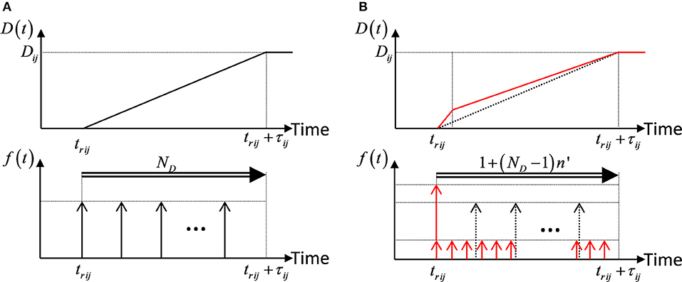
Figure 1. Slip function D(t) and slip correction function f(t), (A) Conventional ones, (B) Revised ones by Irikura (1986).

From these preparations, the ground motion displacement U(t) due to the whole fault may be expressed by

$\begin{array}{cc}\begin{array}{l}U\left(t\right)={\displaystyle \sum _{i=1}^{N_W}{\displaystyle \sum _{j=1}^{N_L}f\left(t-t_{ij}\right)*u_{ij}\left(t\right)}}\\ ={\displaystyle \sum _{i=1}^{N_W}{\displaystyle \sum _{j=1}^{N_L}{\displaystyle \sum _{k=1}^{N_D}{u}_{ij}\left(t-t_{ij}-\left(k-1\right)\frac{{\tau }_{ij}}{N_D}\right)}}}\end{array}& (4)\end{array}$

In this paper, the slip correction function f(t) revised by Irikura (1986) and Yokoi and Irikura (1991) is used and is described by

$\begin{array}{cc}\begin{array}{r}f(t)=\delta (t)+\frac{1}{n^{\prime }}{\displaystyle \sum _{k=1}^{(N_D-1)n^{\prime }}}{u}_{ij}\left(t-\frac{(k-1)\tau }{(N_D-1)n^{\prime }}\right)\end{array}& (5)\end{array}$

Irikura (1986) introduced the number n′ of re-division to remove the effect of artificial periodicity due to the equal-size element division. Figure 1B presents the slip function D(t) and slip correction function f(t) revised by Irikura (1986) and Yokoi and Irikura (1991). Irikura (1994) introduced the following constraint in the setting of n′.

$\begin{array}{cc}\begin{array}{r}\frac{n^{\prime }{N}_D}{\tau }>2f_H\end{array}& (6)\end{array}$

where f_H is the upper bound of the effective frequency.

Finally the ground motion displacement U(t) due to the whole fault can be expressed in terms of the ground motion displacements u_ij(t) due to the fault elements.

$\begin{array}{cc}\begin{array}{l}U\left(t\right)={\displaystyle \sum _i^{N_L}{\displaystyle \sum _j^{N_W}{u}_{ij}\left(t-t_{ij}\right)}}\\ +{\displaystyle \sum _i^{N_L}{\displaystyle \sum _j^{N_W}{\displaystyle \sum _k^{\left(N_D-1\right)n^{\prime }}\frac{1}{n^{\prime }}{u}_{ij}\left(t-t_{ij}-\frac{\left(k-1\right)\tau }{\left(N_D-1\right)n^{\prime }}\right)}}}\end{array}& (7)\end{array}$

The concept of the stochastic Green's function method used in the present study is illustrated in Figure 2.

FIGURE 2

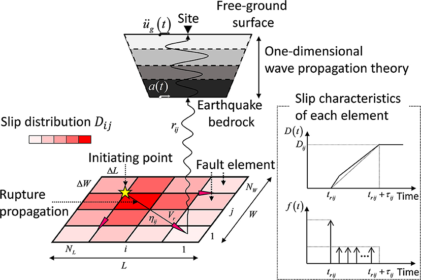
Figure 2. Concept of stochastic Green's function method used in the present study.

Assuming that the fault rupture develops in a concentrically, t_ij can be expressed by

$\begin{array}{cc}\begin{array}{l}{t}_{ij}=t_{pij}+t_{rij}\\ =\frac{r_{ij}}{\beta }+\frac{{\eta }_{ij}}{V_r}\end{array}& (8)\end{array}$

where t_pij: the propagation time from the fault element to the recording point at the earthquake bedrock, t_rij: the slip initiation time in the fault element (the slip initiation time of the initiating point = 0), r_ij: the distance from the fault element to the recording point at the earthquake bedrock, η_ij: the distance from the slip initiation point in the whole fault to the fault element, β : the shear wave velocity of the ground, V_r: the slip propagation speed in the fault.

Small Ground Motion From Element Fault

A small ground motion (acceleration) at the earthquake bedrock due to the slip of a fault element can be derived by setting a point source at the center of the fault element (Boore, 1983). The Fourier amplitude spectrum of the ground motion acceleration at the earthquake bedrock can be expressed by

$\begin{array}{cc}\begin{array}{r}\left|A_{Sij}(\omega )\right|=Source(\omega )·Pass(\omega )\end{array}& (9)\end{array}$

where Source(ω) is the term related to the source (fault) and Pass(ω) is the term related to the wave attenuation in the pass from the fault element to the earthquake bedrock.

In Boore (1983), Source(ω) and Pass(ω) are set as

$\begin{array}{cc}Source\left(\omega \right)=\frac{R_{\theta \varphi }FS·PRTITN}{4\pi \rho {\beta }^3}\left|{\omega }^2\dot{M}\left(\omega \right)\right|& (10)\end{array}$

$\begin{array}{cc}\begin{array}{r}Pass(\omega )=\frac{1}{r_{ij}}exp\left[-\frac{\pi f{r}_{ij}}{Q(f)\beta }\right]\end{array}& (11)\end{array}$

where R_θϕ: radiation pattern coefficient, FS: amplification due to the free surface (= 2), PRTITN: reduction factor that accounts for the partitioning of energy into two horizontal components, ρ : mass density of earthquake bedrock, β : shear wave velocity of earthquake bedrock, Q(f): Q-value. Furthermore, Ṁ(ω) is the source spectrum and is expressed by

$\begin{array}{cc}\left|\dot{M}\left(\omega \right){\left(2\pi f\right)}^2\right|=\frac{M_{0ij}{\left(2\pi f\right)}^2}{1+{\left(f/f_{cij}\right)}^2}P\left(f,f_{\max }\right)& (12)\end{array}$

where M_0ij is the seismic moment of the fault element ij and f_cij is the corner frequency of the fault element ij. P(f, f_max) is a filter for reducing the higher frequency components and is expressed by

$\begin{array}{cc}\begin{array}{r}P(f,f_{max})=\frac{1}{\sqrt{1+{(f/f_{max})}^m}}\end{array}& (13)\end{array}$

where f_max is the cut-off frequency for higher frequency components and m = 4 is assumed according to Boore (1983).

In this paper, the phase difference method due to Yamane and Nagahashi (2008) is used for expressing the phase of ground motion. The standard deviation of the phase difference due to the fault element ijcan be expressed by

$\begin{array}{cc}\begin{array}{r}{\sigma }_{ij}/\pi =0.06+0.0003r_{ij}\end{array}& (14)\end{array}$

This relation refers to inland earthquakes (Makita et al., 2018). In this paper, the near-fault ground motion is assumed in which the effect of the rupture directivity is small. With this standard deviation of the phase difference, the phase spectrum is described by

$\begin{array}{cc}\begin{array}{l}{\varphi }_{k+1ij}={\varphi }_{kij}+\Delta {\varphi }_{kij}(k=1,2,\dots ,N/2-1)\\ \Delta {\varphi }_{ij}=-(\mu +s·{\sigma }_{ij})\end{array}& (15)\end{array}$

where ϕ_kij is the k-th phase spectrum of the fault element ij and Δϕ_kij is the k-th phase difference spectrum of the fault element ij. N is the number of adopted frequencies. Furthermore, μ is the mean of the phase difference and s is the Gaussian random number with 0 mean and unit standard deviation. In this paper, a constant value of μ is assumed in all the fault elements.

The Fourier transform A_Sij(ω) of the acceleration a_Sij(t) at the earthquake bedrock due to the fault element ij can be expressed by

$\begin{array}{cc}\begin{array}{r}{A}_{Sij}(\omega )=\left|A_{Sij}(\omega )\right|·e^{i{\varphi }_{ij}(\omega )}\end{array}& (16)\end{array}$

The inverse Fourier transform of A_Sij(ω) leads to the acceleration a_Sij(t) at the earthquake bedrock due to the fault element ij. Finally, the substitution of this a_Sij(t) into Equation (7) (difference of displacement and acceleration does not matter) provides the acceleration a(t) at the earthquake bedrock due to the whole fault.

Verification of the Method of Ground Motion Generation Using Phase Difference Method

The benchmark test was conducted by Kato et al. (2011) and the model S21 is used for comparison. The benchmark test uses an empirical envelope function of acceleration time histories. On the other hand, the method proposed in this paper employs the phase difference method for representing the phase. Therefore, the proposed method was validated against the above benchmark test. Table 1 shows the similarities and differences between the proposed method and the method used in the benchmark test.

TABLE 1

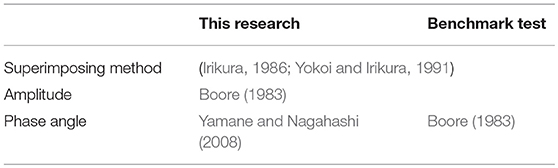
Table 1. Similarities and differences between this research and benchmark test.

The fault plane and three recording points for the model S21 used in the benchmark test Kato et al. (2011) are shown in Figure 3. The recording points are three points (a), (b), (c). The fault plane is assumed to be vertical and the fault type is the right-lateral strike-slip fault. The fault length = 8000m, fault width = 4,000 m, fault slip quantity = 1 m, the seismic moment = $M_0=1.04\times {10}^{18}Nm$, strike angleθ, dip angle δ and rake angle λ are (90°, 90°, 180°). The hypocenter is located at (0, 1,000, 4,000 m) and the fault rupture is propagated concentrically with rupture velocity V_r = 3000(m/s). The hypocenter of each sub-fault is assumed to be located at the center.

FIGURE 3

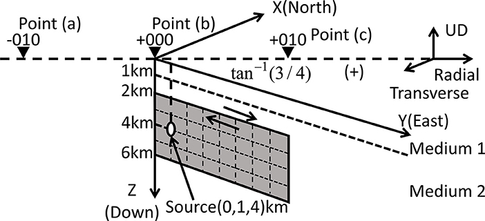
Figure 3. Fault plane and three recording points replotted based on Kato et al. (2011).

In Somerville et al. (1999), Eshelby (1957), and Brune (1970), the area S(km²) of the fault, the stress drop Δσ of large earthquakes and the corner frequency f_c are described by the following equations:

$\begin{array}{cc}\begin{array}{r}S=2.23\times {(M_0\times {10}^7)}^{3/2}\times {10}^{-15}\end{array}& (17)\end{array}$

$\begin{array}{cc}\begin{array}{r}\Delta \sigma =\frac{7}{16}\frac{M_0}{R^3}\times {10}^{-14}\end{array}& (18)\end{array}$

$\begin{array}{cc}\begin{array}{r}{f}_c=4.9·{10}^6{V}_s{\left(\frac{\Delta \sigma }{M_0}\right)}^{1/3}\end{array}& (19)\end{array}$

where R(km) is the effective radius (S = πR²). In these equations, the unit of V_s is km/s, that of Δσ is bar and that of M₀ is dyne-cm.

From Equations (17–19), Δσ = 13.95(Mpa) and f_c = 0.404(Hz) are calculated, then τ = 2/f_c≈5.0(s) is set from Boore (1983). The soil conditions are summarized in Table 2 and the amplification of the ground motion is evaluated by one-dimensional wave propagation theory.

TABLE 2

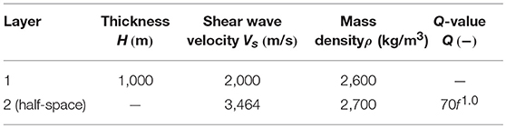
Table 2. Soil conditions.

The fault plane is divided into N_W × N_L elements. N_W = 4 is set in the fault width direction and N_L = 8 is set in the fault length direction. The area of sub-fault is S^S = 1(km²). The seismic moment in each fault element (M_0S) is 5.40 × 10¹⁵Nm and the stress drop (Δσ_S) is assumed to be 13.95(Mpa). The slip D_S of each sub-fault is 0.167(m) from M_0S = μS_SD_S and N_D = 6 from the ratio of fault plane to sub-fault (1/0.167 m). Thus the seismic moment after superimposing the small earthquakes (${M_0}^{\prime }$) is calculated as ${M_0}^{\prime }=N_W·N_L·N_D·M_{0S}\approx 1.04\times {10}^{18}\mathrm{\text{(Nm)}}$, which is the same as M₀. The corner frequency (f_cS) is 2.33 Hz from Equation (19) and the radiation pattern (R_θϕ) is set to 0.63, which is a uniform value in the frequency domain. As for the phase angle, the standard deviation of phase differences (σ_ij/π ) are calculated from Equation (14) and its mean μ/π in each point is set to −0.140 at Point (a), −0.125 at Point (b) and −0.130 at Point (c). Regarding the horizontal component of superimposing wave, only the SH wave is generated by setting PRRITEN to 1 for simplification. Each small earthquake is generated by disassembling into the NS direction component and the EW direction component. Table 3 summarizes the source parameters of the fault plane and sub-faults.

TABLE 3

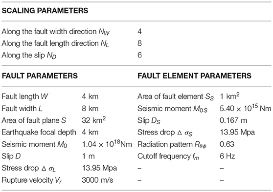
Table 3. Source parameters.

As described above, the amplification of ground motion at the above control points of the soil surface is evaluated by one-dimensional wave propagation theory. In this model, the number of layer is one and the transfer function for describing ground amplification is defined by the following equation:

$\begin{array}{cc}\begin{array}{r}{H}_G(\omega )=\frac{1}{coskH+i\alpha sinkH}\end{array}& (20)\end{array}$

where k, H, and α are the complex wave number, the thickness of layer and the complex impedance, defined by the following equations:

$\begin{array}{cc}\begin{array}{r}k=\omega \sqrt{\rho /G^{*}},G^{*}=(1+2\xi i)G,\alpha =\sqrt{{\rho }_1{G_1}^{*}}/\sqrt{{\rho }_2{G_2}^{*}}\end{array}& (21)\end{array}$

G and G* are the shear modulus and the complex shear modulus. Furthermore ξ is the hysteretic damping ratio of soil. In the benchmark test, ξ = 0 is given. It is noted that, since the radiation damping is taken into account at the earthquake bedrock, the amplification divergence does not occur.

Figure 4 shows the comparison between the proposed method and the abovementioned benchmark test (Kato et al., 2011). The upper one in Figure 4 presents the acceleration at the free ground surface at three points. The lower one in Figure 4 illustrates the pseudo velocity response spectrum. The numbers 1, 2, 3 in figure legend indicate the difference of uniform random numbers for phase angles in Hisada (Kato et al., 2011) and the difference of Gaussian random numbers for phase difference (Equation 15) in Makita et al. (2018). It can be observed from these figures that, while the acceleration time histories exhibit somewhat different properties, especially in its envelope, the pseudo velocity response spectra of both approaches correspond fairly well. This result supports the validity of the method used in this paper. A less-damped response (acceleration time history) by the proposed method with respect to the benchmark test case may result from the fact that, while an envelope function is used in the benchmark test, such function is not used in the proposed method. However, such difference does not cause serious difference in the structural response because the envelope function influences only the initial and ending parts of acceleration time histories with slight effect on the maximum structural response.

FIGURE 4

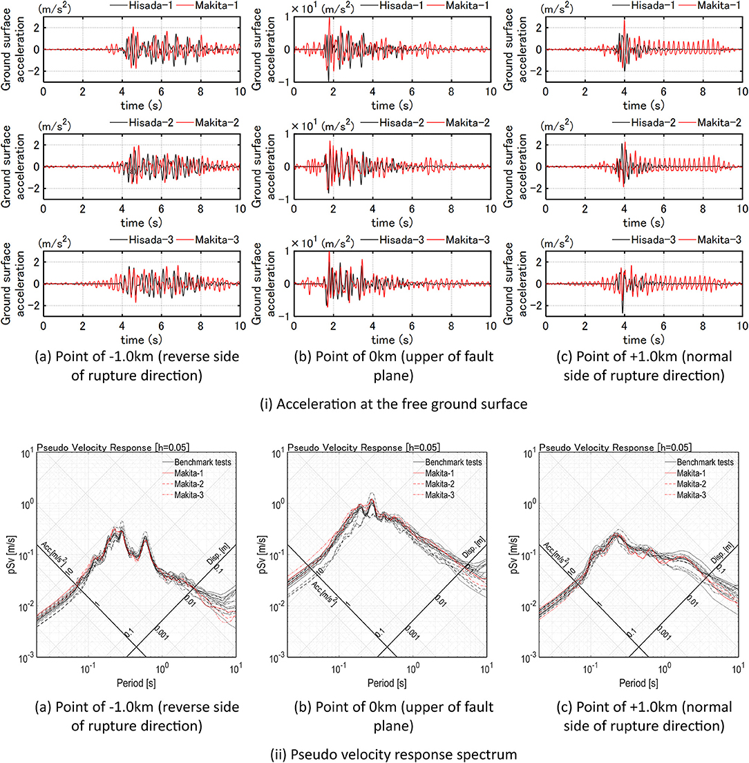
Figure 4. Comparison between the result due to the present method and the result due to the benchmark test [partly from Kato et al. (2011)].

Critical Fault Rupture Slip Maximizing the Structural Response

Concept of Critical Setting of Fault Rupture Slip Distribution and Fault Rupture Front Maximizing the Structural Response at the Earthquake Bedrock and Free-Ground Surface

The soil model and the fault model treated in section Verification of the Method of Ground Motion Generation Using Phase Difference Method (Tables 2, 3) are used again in this section. Although the soil model used in this section (the same as in the benchmark test) seems rather simple, it is noted that the principal objective of this paper is to pay attention to the influence of the fault rupture process on the response of structures on the surface ground. More detailed examination of the effect of the soil properties above the earthquake bedrock will be made in the future as discussed in the previous paper (Makita et al., 2018).

Figure 5 presents the conceptual diagram of the critical setting of the fault rupture slip distribution D_ij and the fault rupture front maximizing the structural response at the earthquake bedrock and free-ground surface (Case A: elastic SDOF model at the earthquake bedrock, Case B: elastic SDOF model at free-ground surface). T is the natural period of the SDOF model and h is the damping ratio. The fault rupture front includes the fault rupture initiation time t_rij (related to the rupture propagation velocity in the fault) and the rise time τ_ij of the slip in each fault element. More specifically, t_rij and τ_ij are treated as independent uncertain parameters in the latter uncertainty modeling. The uncertainty in the fault rupture slip distribution (quantity of slip) for the fixed fault rupture front (concentrically) is treated in section Critical Setting of Fault Rupture Slip Distribution and the uncertainty in the fault rupture front (t_rij and τ_ij) for the fixed fault rupture slip distribution is dealt with in section Critical Setting of Fault Rupture Front.

FIGURE 5

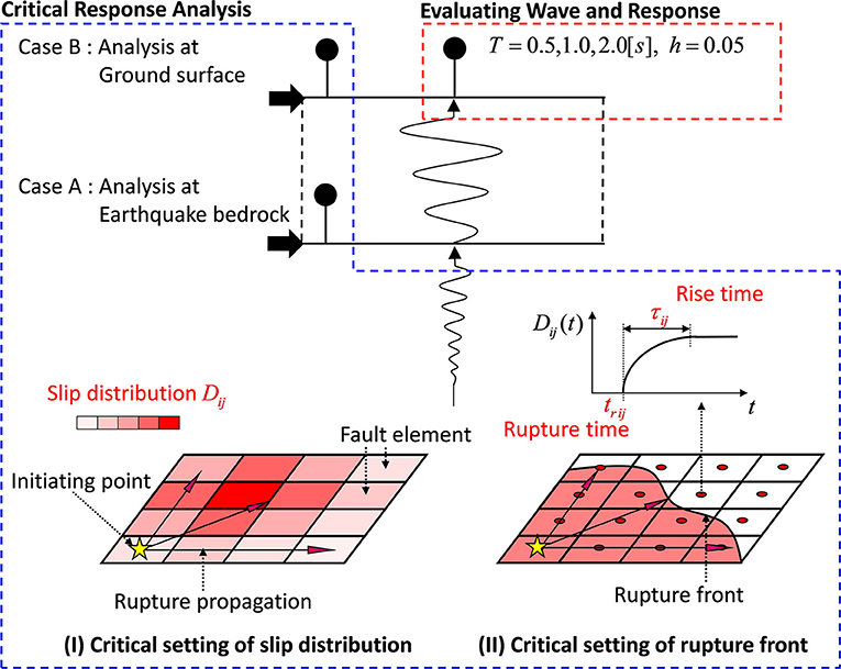
Figure 5. Conceptual diagram of critical setting of fault rupture slip distribution and fault rupture front maximizing the structural response at the earthquake bedrock and free-ground surface (Case A: SDOF model at the earthquake bedrock, Case B: SDOF model at free-ground surface).

A genetic algorithm (GA) has been used for optimization (Goldberg, 1989), i.e., the maximization of the response for uncertain parameters. In this paper, a candidate model of the fault rupture slip distribution or the fault rupture front are treated as chromosomes, and the parameters of each fault element are treated as genes. First, we generate a number of candidate models (first generation), in which fault parameters are changed randomly. Then, we evaluate these models and generate the next generation by selecting elite individuals, do mutation and conduct crossover. In this GA, the Elitist expected value model is used in which the population size is 200, the number of elite individuals is 2 and the probability of crossover is 0.8. It is noted that global and local search of the optimal solution is possible via GA.

Critical Setting of Fault Rupture Slip Distribution

The quantities of the fault rupture slip in fault elements are selected as uncertain parameters. The fault rupture initiation time t_rij and the rise time τ_ij of the slip in each fault element are fixed to the nominal values in this section, i.e., the fault rupture develops from the initiation point concentrically. The ( )^C denotes the nominal value and α is the uncertain parameter. The interval parameters of the fault rupture slip can be expressed by

$\begin{array}{cc}\begin{array}{r}{\text{D}}^I=\left\{\left[{D_{ij}}^C-\alpha \Delta {{\displaystyle \underset{–}{D}}}_{ij},{D_{ij}}^C+\alpha \Delta {\bar{D}}_{ij}\right]\right\}(i=1,\cdots N_W,j=1,\cdots N_L)\end{array}& (22)\end{array}$

The over-bar indicates the upper-side value and the under-bar does the lower-side value. The parameters of the interval analysis are shown in Table 4.

TABLE 4

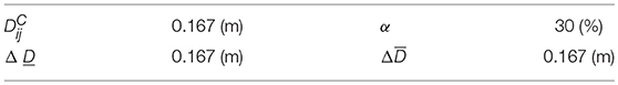
Table 4. Parameters of interval analysis.

In this section, the quantities of the fault rupture slip in fault elements are varying in accordance with the following condition.

$\begin{array}{cc}\begin{array}{l}{\text{D}}^I=\left[D^c-\alpha \Delta {\displaystyle \underset{–}{D}}{D}^c+\alpha \Delta \bar{D}\right]\\ =\left[0.167(m)-0.3\times 0.167(m)0.167(m)+0.3\times 0.167(m)\right]\\ =\left[0.117(m)0.217(m)\right]\end{array}& (23)\end{array}$

Furthermore, the rise time is set to τ = W/(2V_r) = 0.67s from Day (1982) because τ = 5.0s is too long in this model as shown in Kato et al. (2011).

Time–History of Wave

Figure 6 shows the critical ground surface acceleration and deformation of the SDOF model (T = 0.5 s) at three points for Case A (earthquake bedrock motion) and Case B (free-ground surface motion) with respect to uncertain fault rupture slip distribution. Furthermore, Figure 7 presents the critical ground surface acceleration and deformation of SDOF model (T=1.0, 2.0 s) at three points for Case A (earthquake bedrock motion) and Case B (free-ground surface motion).

FIGURE 6

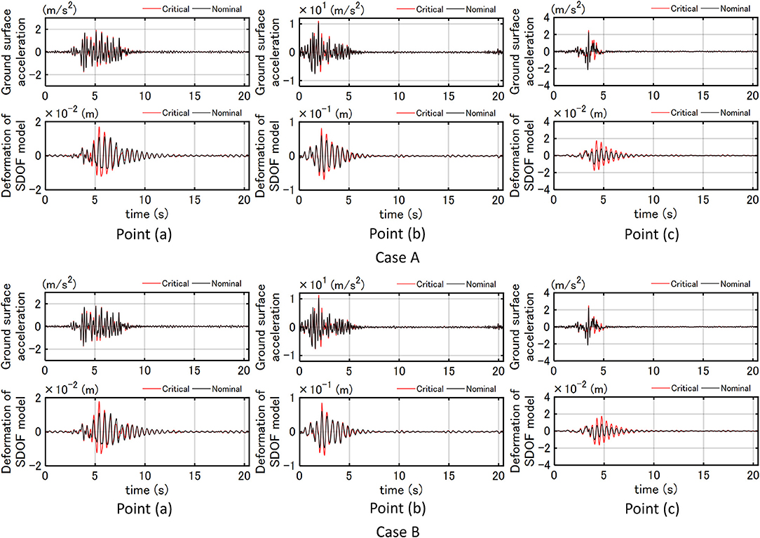
Figure 6. Critical ground surface acceleration and deformation of SDOF model (T = 0.5 s) at three points for Case A (earthquake bedrock motion) and Case B (free-ground surface motion).

FIGURE 7

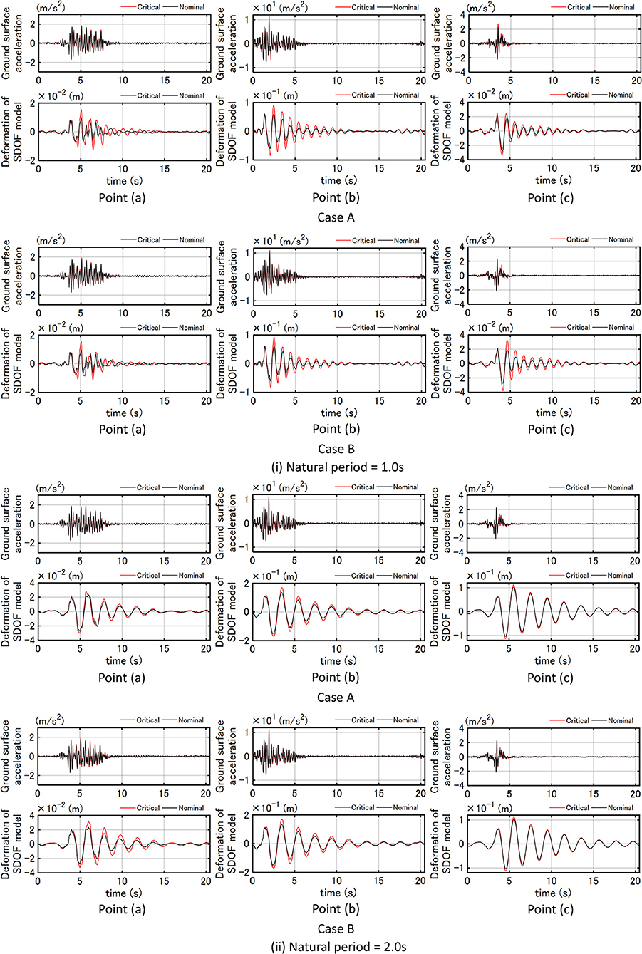
Figure 7. Critical ground surface acceleration and deformation of SDOF model (T = 1.0, 2.0 s) at three points for Case A (earthquake bedrock motion) and Case B (free-ground surface motion).

It can be observed from Figures 6, 7 that the amplification of the ground motion acceleration and the deformation response of the SDOF model of T = 0.5, 1.0 s is larger than those of T = 2.0 s. This means that the effect of the criticality in the uncertainty of the fault rupture slip is larger in the model of shorter natural periods T = 0.5, 1.0 s. In other words, the deviation of structural response between the critical and the nominal case is larger for the natural periods of the SDOF model at T = 0.5 s and T = 1.0 s compared to the case where T = 2.0 s.

Fourier Amplitude Spectrum

Figure 8 shows the Fourier amplitude of critical ground-surface acceleration at three points for three SDOF models (T = 0.5, 1.0, 2.0 s) for Case A (earthquake bedrock motion) and Case B (free-ground surface motion). The broken line indicates the natural frequency of the SDOF model. It can be observed that the Fourier amplitude of critical ground-surface acceleration is amplified much around the natural frequency of the SDOF model. This phenomenon is remarkable in the SDOF model of T = 0.5 s at Point (c). It may be concluded that the critical setting of the fault rupture slip quantity makes the SDOF model resonant to the input.

FIGURE 8

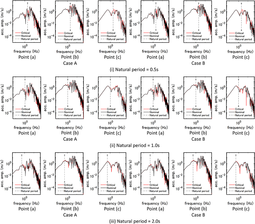
Figure 8. Fourier amplitude of critical ground-surface acceleration at three points for three SDOF models (T = 0.5, 1.0, 2.0 s) for Case A (earthquake bedrock motion) and Case B (free-ground surface motion).

Phase Difference Distribution

Figure 9 presents the phase difference distribution of critical ground-surface acceleration at three points for three SDOF models (T = 0.5, 1.0, 2.0 s) for Case A (earthquake bedrock motion) and Case B (free-ground surface motion). It can be seen that the standard deviation σ/π at Point (c) is the smallest and that at Point (a) is the largest. This may be related to the forward directivity effect. Furthermore σ/π of the critical model is larger than that of the nominal model at Point (b) and that is smaller than that of the nominal model at Point (c) except (i) of Case B. In addition, μ/π of the critical model becomes larger than that of the nominal model. This means that the critical setting of the fault rupture slip quantity makes the acceleration time history delayed.

FIGURE 9

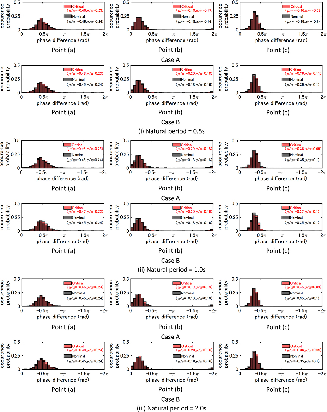
Figure 9. Phase difference distribution of critical ground-surface acceleration at three points for three SDOF models (T = 0.5, 1.0, 2.0 s) for Case A (earthquake bedrock motion) and Case B (free-ground surface motion).

Fault Rupture Slip Distribution

Figure 10 illustrates the fault rupture slip distribution maximizing the response of the three SDOF models (T = 0.5, 1.0, 2.0 s) at three points for Case A (earthquake bedrock motion) and Case B (free-ground surface motion). The seismic moment is indicated at the top of the figures. It can be observed that the seismic moment of the critical fault rupture distribution exhibits a value close to the value for the nominal model $M_0=1.04\times {10}^{18}Nm$. It can also be seen that the critical fault rupture distributions are different in Case A and Case B. This may be because the site amplification is included in Case B in the process of criticality.

FIGURE 10

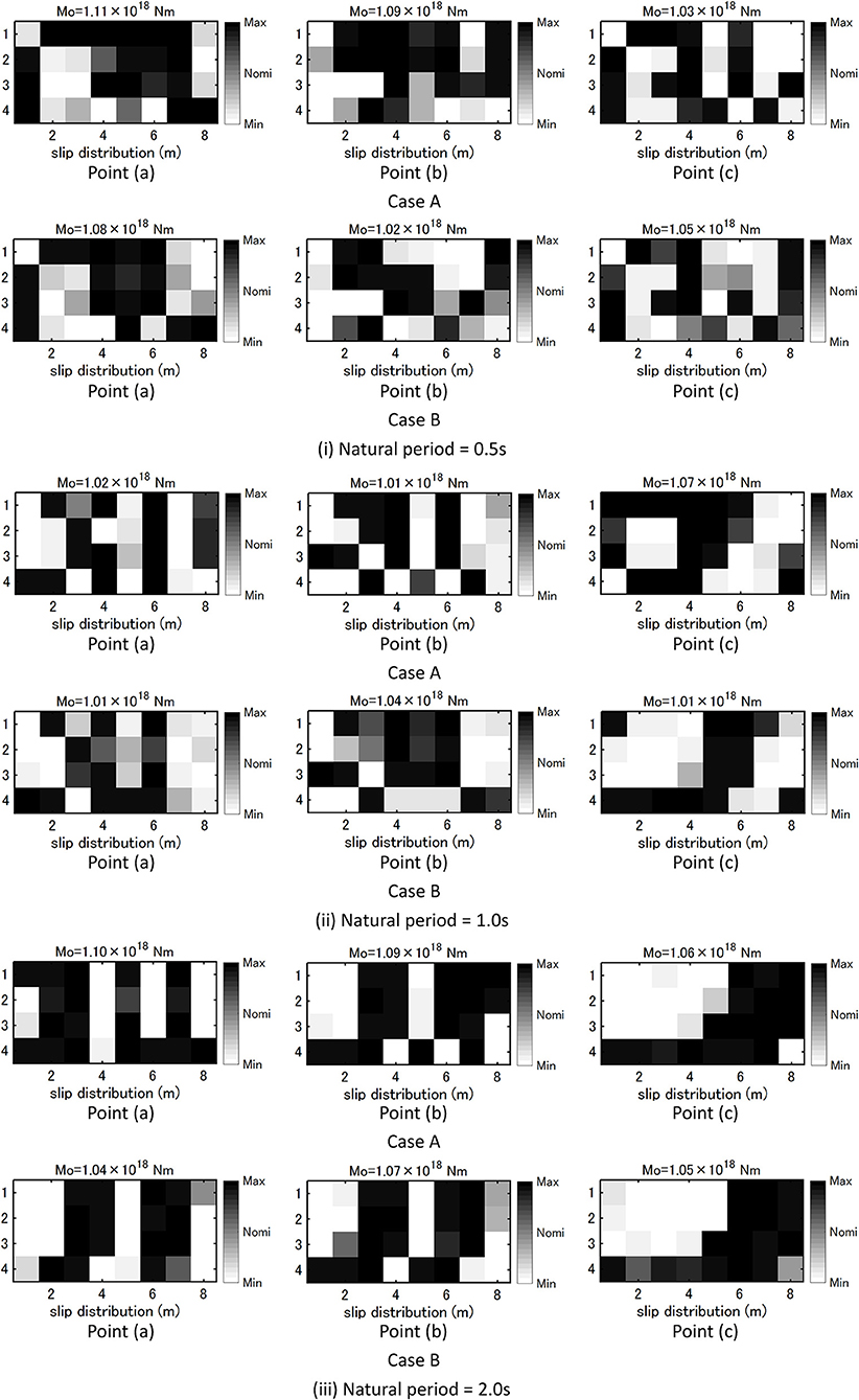
Figure 10. Critical fault rupture slip distribution for three SDOF models (T = 0.5, 1.0, 2.0 s) at three points for Case A (earthquake bedrock motion) and Case B (free-ground surface motion).

Figure 11A shows wave superimposing time t_ij (from the fault rupture initiation in the fault to the arrival at the earthquake bedrock) for each fault element at three points and Figure 11B presents the grouping of fault elements with large slip maximizing the response of two SDOF models (T = 1.0, 2.0 s) at three points for Case B (free-ground surface motion). The triangle in Figure 11A indicates the rupture initiation point and the numbers above Figure 11B indicate the mean of wave superimposing time t_ij at grouping fault elements. It can be observed from Figure 11B that the mean of wave superimposing time t_ij at grouping fault elements is slightly shorter than the natural period of the SDOF model. This may lead to the fact that the acceleration input reflecting the critical fault rupture slip distribution contains the component resonant to the natural period of the SDOF model and amplifies the structural response. In other words, the Fourier amplitude spectrum at the ground surface is amplified in the frequency range of the critical mean of wave superimposing time at grouping fault elements resonant to the natural period of the SDOF model. In addition, the slip of the fault element with the wave superimposing time of 3.71 s becomes large and this may induce a pulse-type wave. Furthermore, the slip distribution in Figure 11B may be regarded as an asperity distribution and this distribution can be used as a tool for setting an asperity in the characteristic model of the fault rupture.

FIGURE 11

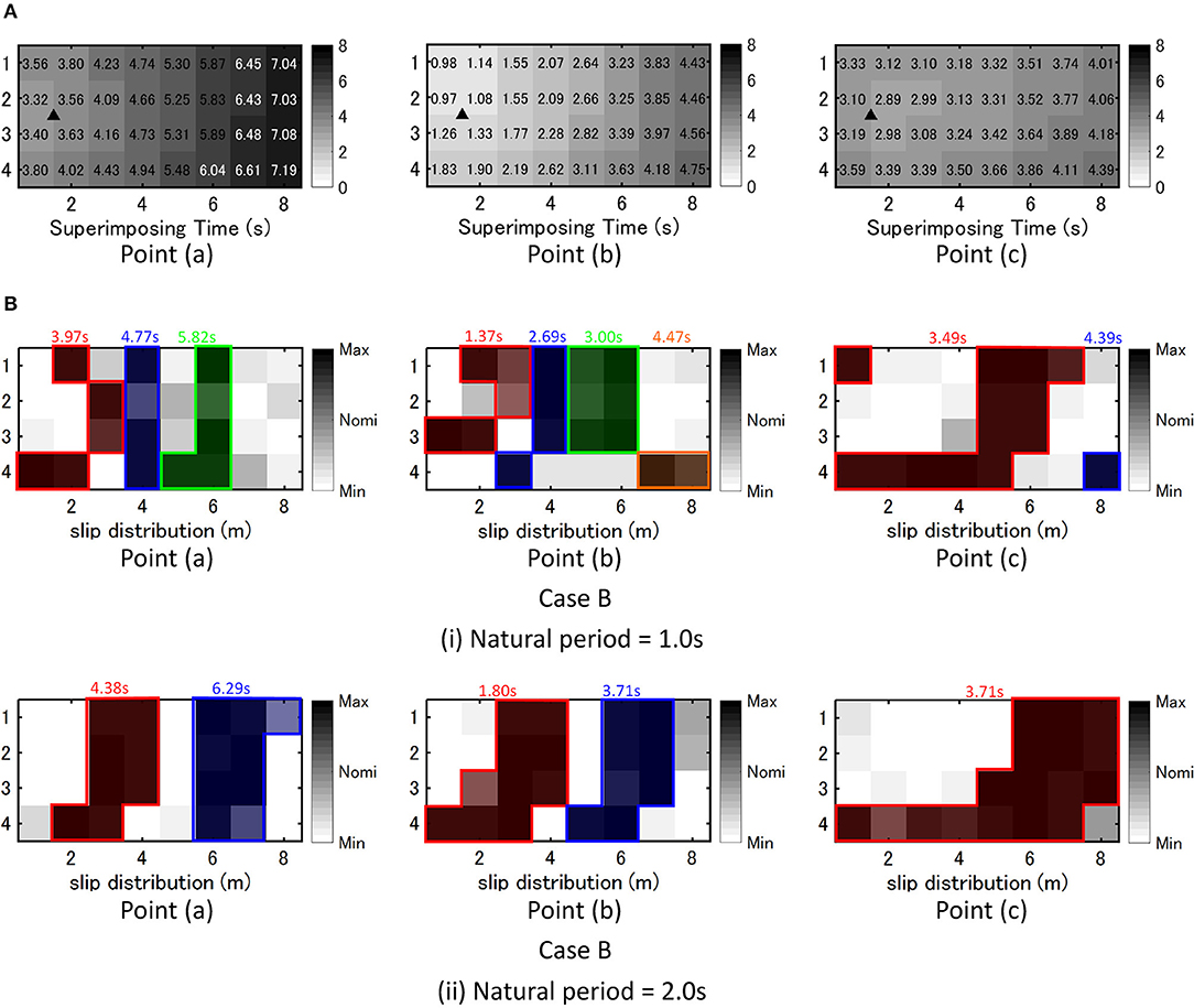
Figure 11. Wave superimposing time t_ij for each fault element and grouping of fault elements with large slip, (A) Wave superimposing time for each fault element at three points for Case A and Case B, (B) Grouping of fault elements with large slip maximizing the response of two SDOF models (T = 1.0, 2.0 s) at three points for Case B (free-ground surface motion).

Critical Setting of Fault Rupture Front

The fault rupture initiation time t_rij and the rise time τ_ij of the slip in each fault element are selected as uncertain parameters. The quantities of the fault rupture slip in fault elements are fixed to the nominal values in this section. ( )^C denotes the nominal value and α is the uncertain parameter. The interval parameters of the fault rupture initiation time and the rise time of the slip can be expressed by

$\begin{array}{cc}\begin{array}{r}{{\text{t}}_{\text{r}}}^I=\left\{\left[{t_{rij}}^C-\alpha \Delta {{\displaystyle \underset{–}{t}}}_{rij},{t_{rij}}^C+\alpha \Delta {\bar{t}}_{rij}\right]\right\}(i=1,\cdots N_W,j=1,\cdots N_L)\end{array}& (24)\end{array}$

$\begin{array}{cc}\begin{array}{r}{{\text{τ}}_{\text{r}}}^I=\left\{\left[{{\tau }_{ij}}^C-\alpha \Delta {{\displaystyle \underset{–}{\tau }}}_{ij},{{\tau }_{ij}}^C+\alpha \Delta {\bar{\tau }}_{ij}\right]\right\}(i=1,\cdots N_W,j=1,\cdots N_L)\end{array}& (25)\end{array}$

where

$\begin{array}{cc}\begin{array}{l}\Delta {{\displaystyle \underset{–}{t}}}_{rij}={t_{rij}}^C,\Delta {\bar{t}}_{rij}={t_{rij}}^C\\ \Delta {{\displaystyle \underset{–}{\tau }}}_{ij}=\Delta {\displaystyle \underset{–}{\tau }}={{\tau }_{ij}}^C,\Delta {\bar{\tau }}_{ij}=\Delta \bar{\tau }={{\tau }_{ij}}^C\end{array}& (26)\end{array}$

As explained before, the over-bar indicates the upper-side value and the under-bar does the lower-side value. Furthermore Δ( ) indicates the parameter for normalization of variation. The parameters for interval analysis is shown in Table 5.

TABLE 5

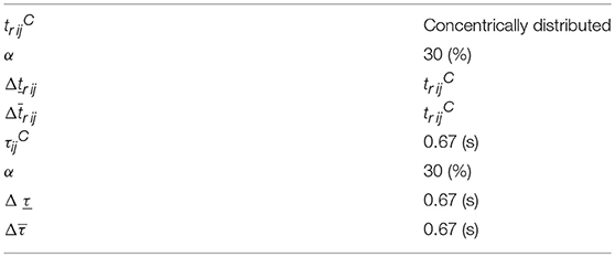
Table 5. Parameters of interval analysis.

Time–History

Figure 12 presents the critical ground surface acceleration and deformation of three SDOF models (T = 0.5, 1.0, 2.0 s) at three points for Case B (free-ground surface motion) with respect to uncertain fault rupture front. It can be observed that the critical acceleration record at Point (c) is amplified much as a pulse-type one and those at Point (a) and (b) are also amplified largely. It can also be seen that, while the uncertainty in the quantity of the fault rupture slip increases the response for the nominal parameters up to about two times as observed in the previous figures, the uncertainty in the rupture propagation velocity in the fault and the rise time of the slip amplifies the response several times. This phenomenon is remarkable in the model of T = 0.5, 1.0 s. However, this is less obvious for T = 2.0 s at Point (c).

FIGURE 12

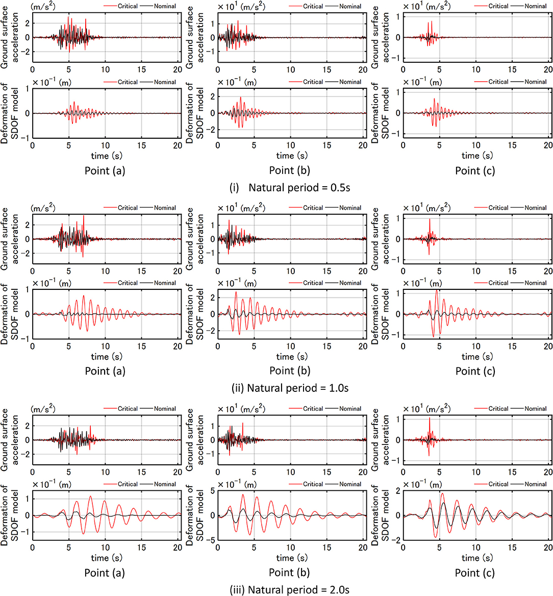
Figure 12. Critical ground surface acceleration and deformation of three SDOF models (T = 0.5, 1.0, 2.0 s) at three points for Case B (free-ground surface motion) with respect to uncertain fault rupture front.

Fourier Amplitude of Ground-Surface Acceleration

Figure 13A presents the Fourier amplitude of ground-surface acceleration at three points maximized for fault rupture front for three SDOF models (T = 0.5, 1.0, 2.0 s) and Case B (maximization for free-ground surface motion). The broken line indicates the natural frequency of the SDOF model. It can be observed that, as seen in the case of the uncertainty in the fault rupture slip, the Fourier amplitude of ground-surface acceleration is amplified much around the natural frequency of the SDOF model. This phenomenon is remarkable at Point (c) and this may be related to the fact that the critical acceleration record at Point (c) is amplified much as a pulse-type one in Figure 12. Furthermore, the amplification is larger than that considering the uncertainty in the quantity of the fault rupture slip. It should be remarked that the natural period of the SDOF model does not coincide with the amplified range of the Fourier amplitude for the model T = 2.0s at Point (c). This may cause the lower response amplification of the model T = 2.0s at Point (c) in Figure 12(iii) than other models.

FIGURE 13

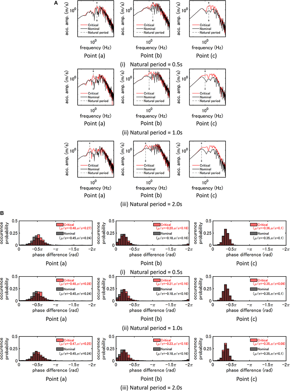
Figure 13. Critical ground surface acceleration at three points with respect to uncertain fault rupture front for three SDOF models (T = 0.5, 1.0, 2.0 s) and Case B (free-ground surface motion), (A) Fourier amplitude, (B) Phase difference distribution.

Phase Difference Distribution

Figure 13B shows the phase difference distribution of ground-surface acceleration at three points maximized for fault rupture front for three SDOF models (T = 0.5, 1.0, 2.0 s) and Case B (free-ground surface motion). It can be seen that the standard deviation σ/π of the critical one is larger than that of the nominal one. On the other hand, the standard deviation σ/π of the critical one becomes smaller than that of the nominal one at Point (c). It may result from the fact that, while the duration time at Point (a) and (b) becomes longer, the duration at Point (c) becomes shorter as a result of pulse-type ground motion. In addition, μ/π becomes larger as a result of criticalization of the rupture front (the uncertainty in the rupture propagation velocity in the fault and the rise time of the slip). This phenomenon was also observed in considering the uncertainty in the quantity of the fault rupture slip.

Critical Fault Rupture Front

Figure 14 presents the wave superimposing time t_ij (from the fault rupture initiation in the fault to the arrival at the earthquake bedrock) at each fault element and the rise time τ_ij at each fault element characterizing the critical fault rupture front maximized for three points and three SDOF models (T = 0.5, 1.0, 2.0 s) corresponding to Case B (free-ground surface motion). The triangle in Figure 14 indicates the rupture initiation point. It can be observed from Figure 14A that the fault element rupture occurs in a concentrated manner corresponding to the time interval of the natural period of the SDOF model. In addition, the rupture directivity effect can be observed in the model of T = 1.0, 2.0 s at Point (c) and it may be related to the fact that the pulse-type input induces larger responses. Furthermore, it can be observed from Figure 14B that, while the rate of τ_ij around the nominal value is large in the model of T = 0.5 s, τ_ij moves to the lower limit around τ_ij = 0.47–0.49 s in the model of T = 1.0, 2.0 s.

FIGURE 14

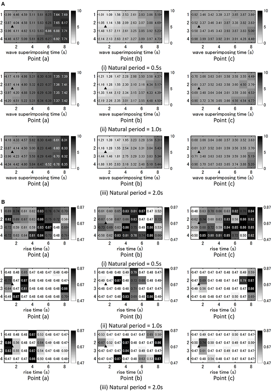
Figure 14. Critical fault rupture front obtained for three points and three SDOF models (T = 0.5, 1.0, 2.0 s) corresponding to Case B (free-ground surface motion), (A) wave superimposing time t_ij at each fault element, (B) Rise time τ_ij at each fault element.

Robustness Evaluation for Uncertain Fault Rupture Slip Distribution and Uncertain Fault Rupture Front

Figure 15A shows the robustness function $\widehat{\alpha }$, proposed by Ben-Haim (2006), with respect to the deformation of the SDOF model for uncertain parameters of quantity of fault rupture slip for Case (B). Once the value $\widehat{\alpha }$ in the vertical axis is fixed, the corresponding deformation of the SDOF model in the horizontal axis indicates the maximum value for varied uncertain parameters (quantity of fault rupture slip) prescribed by $\widehat{\alpha }$. In particular, the deformation of the SDOF model for $\widehat{\alpha }=0$ indicates the maximum response for the nominal parameters. It can be observed that the robustness becomes the smallest for the model at Point (b). This is because the response of the SDOF model is the largest at Point (b). The slope of the robustness function indicates the degree of the robustness. As the slope becomes steeper, the model becomes more robust.

FIGURE 15

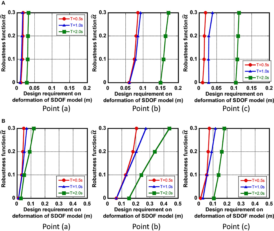
Figure 15. Robustness function with respect to deformation of three SDOF models (T = 0.5, 1.0, 2.0 s) at three points corresponding to Case B (free-ground surface motion), (A) Uncertain quantity of fault rupture slip, (B) Uncertain quantity of fault rupture front.

Figure 15B presents the robustness function $\widehat{\alpha }$ with respect to the deformation of the SDOF model for uncertain parameters of fault rupture front (slip initiation time and rise time) for Case (B). Once the value $\widehat{\alpha }$ in the vertical axis is fixed, the corresponding deformation of the SDOF model in the horizontal axis indicates the maximum value for varied uncertain parameters (slip initiation time and rise time) prescribed by $\widehat{\alpha }$. It can be observed that the robustness becomes the smallest for the model at Point (b) as in Figure 15A. Compared to the case in Figure 15A, the slope of the robustness function becomes small.

Since the robustness is closely related to the resilience, the presented method using the robustness function seems useful for the evaluation of resilience of buildings against uncertain fault rupture slip distribution and uncertain fault rupture front.

Conclusions

To promote a new methodology for resilient building design, a critical excitation method has been proposed in which the whole process of theoretical ground motion generation is treated. The process consists of (i) the fault rupture process, (ii) the wave propagation from the fault to the earthquake bedrock, (iii) the site amplification. The uncertainty in the fault rupture slip has been dealt with in the present paper, i.e., the quantity of the fault rupture slip, the rupture propagation velocity in the fault and the rise time of the slip. The wave propagation from the fault to the earthquake bedrock has been expressed by the stochastic Green's function method in which the Fourier amplitude at the earthquake bedrock from a fault element has been represented by the Boore's model and the phase angle has been modeled by the phase difference method. The validity of the proposed method has been investigated through the comparison with the existing simulation result by other methods incorporating the empirical envelope function of acceleration time histories. By using the proposed method for ground motion generation and for optimization under uncertainty in the fault rupture slip, a methodology has been presented for deriving the critical ground motion causing the maximum response of an elastic SDOF model at the earthquake bedrock or at the free ground surface. A genetic algorithm (GA) has been used for optimization, i.e., the maximization of the response for uncertain parameters. The following conclusions have been derived.

(1) While the uncertainty in the quantity of the fault rupture slip increases the response for the nominal parameters up to about two times, the uncertainty in the rupture propagation velocity in the fault and the rise time of the slip amplifies the response up to 1.7–8.0 times.

(2) The response at the epicenter becomes larger than that at other recording point.

(3) The setting of the objective function for criticality, i.e., the maximum response of an elastic SDOF model at the earthquake bedrock or at the free ground surface, does not affect largely the result of the critical excitation problem. In other words, the ground above the earthquake bedrock plays a role as a filter of ground motions and it does not affect the critical nature of ground motions at the earthquake bedrock.

Since the critical ground motion produces the worst building response among possible scenarios, the proposed method can be a reliable tool for resilient building design.

Author Contributions

KM formulated the problem, conducted the computation, and wrote the paper. KK conducted the computation and discussed the results. IT supervised the research and wrote the paper.

Conflict of Interest Statement

The authors declare that the research was conducted in the absence of any commercial or financial relationships that could be construed as a potential conflict of interest.

Acknowledgments

Part of the present work is supported by KAKENHI of Japan Society for the Promotion of Science (No. 17K18922, 18H01584). This support is greatly appreciated.

References

Abrahamson, N., Ashford, S., Elgamal, A., Kramer, S., Seible, F., and Somerville, P. (1998). Proceedings of the 1st PEER Workshop on Characterization of Special Source Effects (San Dieg, CA: Pacific Earthquake Engineering Research Center, University of California).

Google Scholar

Ben-Haim, Y. (2006). Info-Gap Decision Theory: Decisions Under Severe Uncertainty, 2nd Edn. London: Academic Press.

Google Scholar

Boore, D. M. (1983). Stochastic simulation of high-frequency ground motions based on seismological models of the radiated spectra. Bull. Seismol. Soc. Am. 73, 1865–1894.

Google Scholar

Bouchon, M. (1981). A simple method to calculate Green's functions for elastic layered media. Bull. Seismol. Soc. Am. 71, 959–971.

Google Scholar

Brune, J. N. (1970). Tectonic stress and the spectra of seismic shear waves from earthquakes. J. Geophys. Res. 75, 4997–5009. doi: 10.1029/JB075i026p04997

CrossRef Full Text | Google Scholar

Cotton, F., Archuleta, R., and Causse, M. (2013). What is sigma of the stress drop? Seismol. Res. Lett. 84, 42–48. doi: 10.1785/0220120087

CrossRef Full Text | Google Scholar

Day, S. M. (1982). Three-dimensional finite difference simulation of fault dynamics: rectangular fault with fixed rupture velocity. Bull. Seismol. Soc. Am. 72, 83–96.

Google Scholar

Drenick, R. F. (1970). Model-free design of aseismic structures. J. Eng. Mech. Div. ASCE 96, 483–493.

Google Scholar

Eshelby, J. D. (1957). The determination of the elastic field of an ellipsoidal inclusion and related problems. Proc. R. Soc. A 241, 376–396. doi: 10.1098/rspa.1957.0133

CrossRef Full Text | Google Scholar

Fukumoto, Y., and Takewaki, I. (2017). Dual control high-rise building for robuster earthquake performance. Front. Built Environ. 3:12. doi: 10.3389/fbuil.2017.00012

CrossRef Full Text | Google Scholar

Goldberg, D. E. (1989). Genetic Algorithms in Search, Optimization, and Machine Learning. Boston, MA: Addison–Wesley.

Google Scholar

Hisada, Y. (2008). Broadband strong motion simulation in layered half-space using stochastic Green's function technique. J. Seismol. 12, 265–279. doi: 10.1007/s10950-008-9090-6

CrossRef Full Text | Google Scholar

Hisada, Y., and Bielak, J. (2003). A theoretical method for computing near-fault ground motions in layered half-spaces considering static offset due to surface faulting with a physical interpretation of fling step and rupture directivity. Bull. Seismol. Soc. Am. 93, 1154–1168. doi: 10.1785/0120020165

CrossRef Full Text | Google Scholar

Irikura, K. (1983). Semi-empirical estimation of strong ground motions during large earthquakes. Bull. Disaster Prev. Res. Inst. 33, 63–104.

Google Scholar

Irikura, K. (1986). “Prediction of strong acceleration motions using empirical Green's function,” in Proceedings of the 7th Japan Earthquake, Engineering Symposium (Tokyo). 151–156.

Google Scholar

Irikura, K. (1994). Earthquake source modeling for strong motion prediction. J. Seismol. Soc. Jpn. 46, 495–512.

Google Scholar

Kasagi, M., Fujita, K., Tsuji, M., and Takewaki, I. (2016). Automatic generation of smart earthquake-resistant building system: hybrid system of base-isolation and building-connection. Heliyon 2:e00069. doi: 10.1016/j.heliyon.2016.e00069

PubMed Abstract | CrossRef Full Text | Google Scholar

Kato, K., Hisada, Y., Kawabe, H., Ohno, S., Nozu, A., Nobata, A., et al. (2011). Benchmark tests for strong ground motion prediction methods: case for stochastic Green's function method (Part1). J. Technol. Design AIJ 17, 49–54. doi: 10.3130/aijt.17.49

CrossRef Full Text | Google Scholar

Lawrence Livermore National Laboratory (2002). Guidance for Performing Probabilistic Seismic Hazard Analysis for a Nuclear Plant Site: Example Application to the Southeastern United States. NUREG/CR-6607, UCRL-ID-133494.

Makita, K., Murase, M., Kondo, K., and Takewaki, I. (2018). Robustness evaluation of base-isolation building-connection hybrid controlled building structures considering uncertainties in deep ground. Front. Built Environ. 4:16. doi: 10.3389/fbuil.2018.00016

CrossRef Full Text | Google Scholar

Morikawa, N., Kanno, T., Narita, A., Fujiwara, H., Okumura, T., Fukushima, Y., et al. (2008). Strong motion uncertainty determined from observed records by dense network in Japan. J. Seismol. 12, 529–546. doi: 10.1007/s10950-008-9106-2

CrossRef Full Text | Google Scholar

Murase, M., Tsuji, M., and Takewaki, I. (2013). Smart passive control of buildings with higher redundancy and robustness using base-isolation and inter-connection. Earthquakes Struct. 4, 649–670. doi: 10.12989/eas.2013.4.6.649

CrossRef Full Text | Google Scholar

Murase, M., Tsuji, M., and Takewaki, I. (2014). Hybrid system of base isolation and building connection for control robust for broad type of earthquake ground motions. J. Struct. Eng. AIJ 60B, 413–422.

Google Scholar

Nickman, A., Hosseini, A., Hamidi, J. H., and Barkhordari, M. A. (2013). Reproducing fling-step and forward directivity at near source site using of multi-objective particle swarm optimization and multi taper. Earthquake Eng. Eng. Vibrat. 12, 529–540.

Google Scholar

Okada, T., Fujita, K., and Takewaki, I. (2016). Robustness evaluation of seismic pile response considering uncertainty mechanism of soil properties. Innovat. Infrastruct. Solut. 1:5. doi: 10.1007/s41062-016-0009-8

CrossRef Full Text | Google Scholar

Somerville, P., Irikura, K., Graves, R., Sawada, S., Wald, D., Anderson, N., et al. (1999). Characterizing crustal earthquake slip models for the prediction of strong ground motion. Seismol. Res. Lett. 70, 59–80. doi: 10.1785/gssrl.70.1.59

CrossRef Full Text | Google Scholar

Takewaki, I. (2007). Critical Excitation Methods in Earthquake Engineering, 2nd Edn. London: Elsevier.

Google Scholar

Taniguchi, M., and Takewaki, I. (2015). Bound of earthquake input energy to building structure considering shallow and deep ground uncertainties. Soil Dyn. Earthquake Eng. 77, 267–273. doi: 10.1016/j.soildyn.2015.05.011

CrossRef Full Text | Google Scholar

Wennerberg, L. (1990). Stochastic summation of empirical Green's functions. Bull. Seismol. Soc. Am. 80, 1418–1432.

Google Scholar

Yamane, T., and Nagahashi, S. (2008). “A generation method of simulated earthquake ground motion considering phase difference characteristics,” in Proceedings of the 14th World Conference on Earthquake Engineering (Beijing).

Google Scholar

Yokoi, T., and Irikura, K. (1991). Empirical Green's function technique based on the scaling law of source spectra. J. Seism. Soc. Jpn. 44, 109–122. doi: 10.4294/zisin1948.44.2_109

CrossRef Full Text | Google Scholar

Yoshimura, C., Bielak, J., Hisada, Y., and Fernandez, A. (2003). Domain reduction method for three-dimensional earthquake modeling in localized regions, Part II: verification and applications. Bull. Seismol. Soc. Am. 93, 825–840. doi: 10.1785/0120010252

CrossRef Full Text | Google Scholar