Predicting Roof Pressures on a Low-Rise Structure From Freestream Turbulence Using Artificial Neural Networks

Introduction

Boundary layer wind tunnel (BLWT) testing is still considered the primary experimental instrument to accurately reproduce and assess wind-induced loads on building structures. The continued dependence on wind tunnels is ascribed, in part, to the inability of computational (e.g., CFD) methods to accurately capture local pressure fields in flow separating regions around sharp edged bluff bodies (Ricci et al., 2017); these regions typically produce the largest peak loads on low-rise structures. Furthermore, prior experimental work (e.g., Hillier and Cherry, 1981; Gartshore, 1984; Saathoff and Melbourne, 1997; Akon and Kopp, 2016) in BLWTs has revealed the strong influence of the turbulence characteristics of the incident flow on the spatial distribution of local pressures near separating shear layers developed around surface-mounted prisms (e.g., low-rise structures). These localized pressure fields directly affect the overall (i.e., global) flow organization, which often leads to inaccuracies in numerical (e.g., LES) results when attempting to recreate the flow behavior around sharp-edged bluff bodies; even when simple geometries are considered (e.g., Bruno et al., 2014). Alternatively, BLWTs experiments have proven to be an effective tool for properly simulating the turbulence properties of approach flows and accurately capturing the complex pressure fields acting on sharp-edged bluff bodies. Yet, due to cost and time constraints, experiments in the BLWT commonly entail a limited number of building configurations and approach flow conditions. To address gaps in experimental databases, this study makes use of existing experimental BLWT datasets and artificial neural networks (ANN) to assist in the development of robust and reliable mathematical models for accurately quantifying peak wind loading on low-rise structures and their inherent dependence on freestream turbulent flows.

Adequate assessment of wind-induced loads in the BLWT requires proper simulation of the turbulent structures present in the lower part of the atmospheric boundary layer (ABL). In the case of low-rise structures, previous studies have suggested that achieving the desired full-scale turbulence characteristics at (or near) the model height is one of the main requirements for accurately quantifying the magnitude and distribution of surface pressures in separated flow regions (Tieleman et al., 1978; Tieleman, 1992; e.g., St. Pierre et al., 2005); flow parameters, such as the roughness length and the displacement height are often poor indicators of the local pressure fields in the separated flow region. Akon and Kopp (2016) investigated the structure of the separation bubble near the leading edge of the roof of a generic low-rise building model immersed in several turbulent boundary layer flows. They found that the turbulence properties of the approaching flow affected both the pressure distributions and the mean size of the separation bubble. Subsequently, Fernández-Cabán and Masters (2018) independently confirmed these observations through a comprehensive series of BLWT experiments for a family of boundary layer flows. The two studies focused on approach flows acting parallel and perpendicular to the building faces; i.e., cornering wind directions were not investigated.

The present work aims at developing a generalized high-fidelity approach to accurately predict (i.e., interpolate) the distribution of surface pressures near separated flow regions on a low-rise structure based on freestream turbulent flow conditions. A robust feed-forward multilayer artificial neural network (ANN) using a backpropagation (BP) training algorithm is employed to analytically predict the mean, RMS, and peak pressure coefficients on the roof of a low-rise structure given the freestream turbulence intensity (at eave height) and the normalized plan roof coordinates. A robust feed-forward multilayer artificial neural network (ANN) using a backpropagation (BP) training algorithm is employed. ANNs are biologically inspired mathematical models well-suited for solving non-linear multivariate modeling problems. ANNs generate complex functional relationships (Turkkan and Srivastava, 1995) to produce analytical models through training using experimental (or computational) datasets, even when given noisy or incomplete information (Haykin, 1994), thus providing a resourceful alternative to other multivariate/non-linear interpolation techniques, such as regression polynomials and kriging methods (Franke, 1982).

Several works can be found in literature which apply ANNs for characterizing wind load effects on building structures. For instance, Chen et al. (2003) employed a backpropagation training algorithm to predict mean and root-mean-square (RMS) pressures acting on gable roofs of low-rise buildings. Subsequently, Gavalda et al. (2011) further expanded on this work by presenting an ANN driven interpolation methodology that incorporated variable plan dimensions and roof slopes. Additionally, a fuzzy neural network (FNN) approach was developed in Fu et al. (2006) for the prediction of mean pressure distributions and power spectra of fluctuating wind pressures on a cantilevered flat roof. The use of ANNs have also been examined in the evaluation of tall wind-exited buildings. For example, Zhang and Zhang (2004) applied a radial basis function (RBF) neural network to predict and analyze wind-induced interference effects from surrounding obstructions on tall buildings. More recently, Dongmei et al. (2017) coupled a backpropagation neural network (BPNN) with proper orthogonal decomposition (POD-BPNN) for the prediction of wind-induced mean and RMS pressures acting on the surface of a high-rise building. The current work further exploits the capabilities of ANNs by integrating upwind terrain parameters into a network to produce functional relationships between the turbulence features of the approaching flow and the peak pressure loading on bluff bodies.

A large dataset comprising an extensive series of aerodynamic pressure tests conducted in a large BLWT was utilized for training, validation, and testing the ANN model. The dataset encompasses 33 different terrains, three building model scales (1:20, 1:30, and 1:50) and three wind directions (parallel and perpendicular to the ridgeline and cornering), which equates to nearly 300 independent experiments. The present work focuses on the cornering (i.e., 45°) wind direction, critical for roof suction pressures. The 33 upwind terrains simulate approach flow conditions ranging from marine (i.e., smooth) to dense suburban exposures.

The predictive capabilities of ANN can supplant the need for additional experiments to investigate terrain effects in the BLWT, which typically entail laborious and time consuming alterations of the upstream terrain (e.g., roughness grid) to achieve targeted roughness parameters and turbulent characteristics at the test section. In addition, the approach can be used to further expand existing aerodynamic databases; which commonly cover a limited number of upwind terrain conditions (e.g., open and suburban); and provide a tool for design practitioners to rapidly and reliably quantify the effects of changes in upstream terrain and extreme pressure loading acting on low-rise structures.

Experimental Dataset

The experimental dataset applied in this study comprises a series of BLWT pressure tests conducted on a 1:20, 1:30, and 1:50 scaled rigid building models of the Wind Engineering Research Field Laboratory (WERFL; Levitan and Mehta, 1992a,b) experimental building. The complete dataset is publicly accessible through the Natural Hazard Engineering Research Infrastructure (NHERI) DesignSafe cyberinfrastructure web-based research platform (Fernández-Cabán and Masters, 2017; dataset). BLWT experiments were conducted at the University of Florida (UF) NHERI Experimental Facility. The UF BLWT is a low-speed open circuit tunnel with dimensions of 6 m W × 3 m H × 38 m L. The maximum blockage ratio in the tunnel was <0.8%. A more detailed description of the UF BLWT can be found in Fernández-Cabán and Masters (2018).

Model Geometry, Tap Layout, and Pressure Measurements

The three WERFL building models were instrumented with 266 pressure taps; 152 roof taps and 114 wall taps. The tap location followed the layout used in the 1:100 WERFL building model of the NIST aerodynamic database (Ho et al., 2003; Test 7, ST3/ST4), however 60 additional taps were added on the roof of the model to improve the spatial resolution of the pressure field in this region, as shown in Figure 1. The plan dimensions in Figure 1 are shown in terms of the eave height of the model H. The full-scale dimensions of the WERFL building are 45 ft [13.7 m] × 30 ft [8.9 m] × 13 ft [3.96 m] ($\frac{1}{4}$:12 roof slope; i.e., aerodynamically flat). A cornering (α = 45°) wind direction was considered in this study.

FIGURE 1

Figure 1. Pressure tap layout on the roof of the three UF WERFL building models. Tap ID and (normalized) coordinates follow the layout of Test 7 (ST3/ST4) of the NIST aerodynamic database. The red “x” markers represent additional taps that were added to the original layout (blue “o” markers).

Simultaneous pressure measurements were recorded using eight high-speed electronic pressure scanning modules from Scanivalve ZOC33 (Scanivalve, 2016). Pressure taps were connected to the modules using 122 cm long urethane tubing. Pressure coefficients shown in this paper are computed as the ratio of the differential pressure and the mean velocity (dynamic) pressure at the eave height of the model:

$\begin{array}{rc}{C}_p(t)=\frac{p(t)-p_0}{1/2\rho U_H^2}& (1)\end{array}$

where p(t) is the (absolute) pressure measured, p₀ is the reference (static) pressure, ρ is the air density, and U_H is the mean streamwise velocity at eave height estimated from the mean reference velocity pressure in the freestream at z = 1.48 m above the floor. The reference velocity pressure was converted to the eave height of the building model using an empirical adjustment factor (k) obtained from flow measurements with the model removed; U_H = kU_ref, where U_ref is the mean velocity at z = 1.48 m. Static reference pressures (p₀) were taken from the static port of the Pitot tube to ensure stable measurements with negligible fluctuations. Air density (ρ) was calculated from the air temperature, barometric pressure, and relative humidity measured during each test.

The pressure signals were digitally filtered to remove resonance and damping effects in the tubes (Irwin et al., 1979) using transfer functions following the approach described in Pemberton (2010). The test durations for the 1:20, 1:30, and 1:50 models were 300, 180, and 120 s, respectively. These equate to a full-scale duration of ~30 min for the three models—assuming a 1/3.33 velocity scale. Data was recorded at sampling rate of 625 Hz. The pressure measurements in the dataset are digitally filtered using a third order Butterworth low-pass filter with a cutoff frequency of 200 Hz.

Terrain Simulation

Simulation of upwind terrain roughness is achieved through the Terraformer, an automated roughness element grid that rapidly reconfigures the height and orientation of 1,116 roughness elements in a 62 × 18 grid to produce desired upwind terrain conditions along an 18.3 m fetch (Fernández-Cabán and Masters, 2018). Roughness elements are 5 × 10 cm in plan, and are spaced 30 cm apart in a staggered arrangement. Height and orientation can be varied from 0–160 mm and 0–360 degrees, respectively. The turbulence properties of the approach flow at the test section were varied by adjusting the configuration of the Terraformer upwind of the model. Wide and narrow edge windward element orientations were applied (Figure 2). Roughness elements were elevated from h = 0 mm−160 mm using increments of 10 mm, thus producing 16 upwind terrain conditions for each element orientation; totaling 33 terrains including the base floor (i.e., flush) case. Reynolds number (Re = HU_H/ν) ranged from 3.2 × 10⁴ (U_H~6 m/s and H = 79.2 mm; 1:50 model) to 14.9 × 10⁴ (U_H~11.4 m/s and H = 198 mm; 1:20 model). Table 1 summarizes the freestream turbulence levels at the eave height of the models for the range of roughness element heights and orientations examined.

FIGURE 2

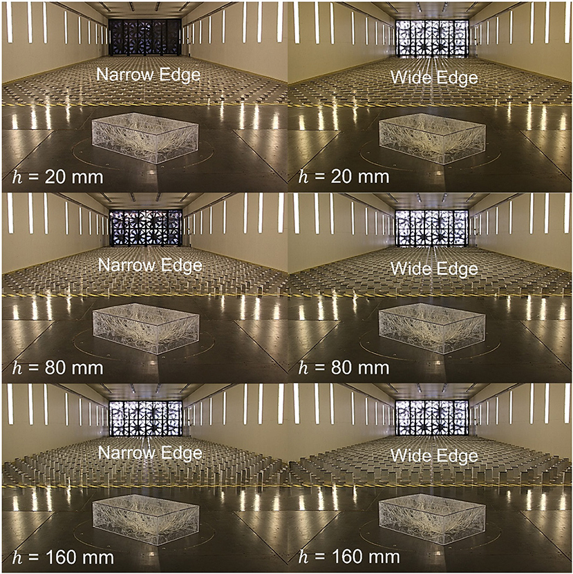
Figure 2. Six representative upwind terrain configurations for the UF 1:20 WERFL building model oriented at a 45° (cornering) wind direction.

TABLE 1

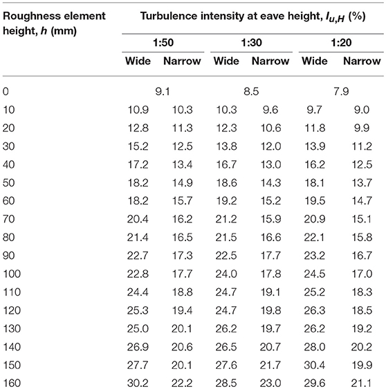
Table 1. Longitudinal turbulence intensities of the freestream measured at the eave height of the 1:50, 1:30, and 1:20 building models.

Figure 3 illustrates two representative longitudinal turbulence spectra of the freestream measured at eave height of the model z = H; H = 79.2, 132, 198 mm for the 1:50, 1:30, and 1:20 models, respectively; for sparse and dense open terrain simulations. Measurements were collected at the center of the test section using Cobra velocity probes with the model removed. The spectra are normalized by the squared of the mean velocity (U²) at z = H. The von Karman spectrum—adopted in ESDU 83045 (1983)—was fitted to the data using equivalent full-scale roughness lengths z₀ = 0.01 and 0.087 m. These roughness lengths represent the two WERFL site conditions (i.e., exposures) examined for the 1:100 WERFL model in the NIST aerodynamic database; z₀ = 0.01 m (ST3) and z₀ = 0.087 m (ST4). The sparse open exposure was achieved in the UF BLWT for a roughness element height h = 40 mm while h = 90 mm produced the dense open terrain simulation. Both examples used the wide edge windward element orientation in the Terraformer.

FIGURE 3

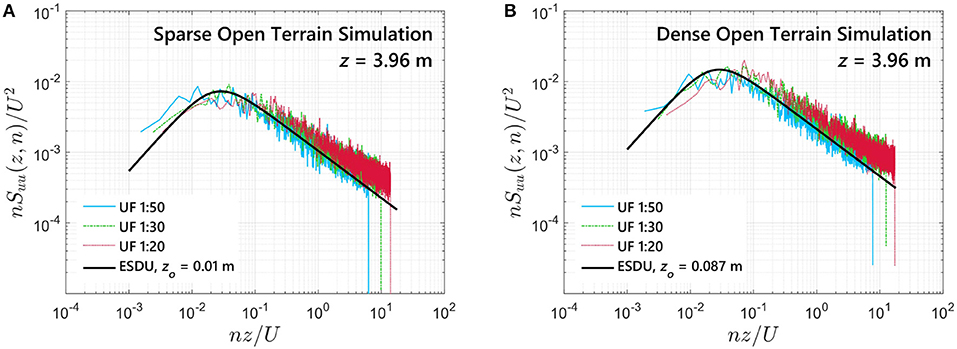
Figure 3. Longitudinal turbulence spectra; at eave height (z = 3.96 m full-scale); of the freestream measured at the center of the test section; with the building model removed. The simulation of the two terrains is achieved for roughness element heights of 40 mm (sparse open) and 100 mm (dense open) in a wide edge windward orientation.

Artificial Neural Networks (ANNs)

ANNs are biologically inspired mathematical methods which loosely resemble the complex functions of the human brain for learning and pattern recognition (Nasrabadi, 2007). Common ANN systems contain a collection of interconnected parallel processing units, called neurons. These neurons can store experimental knowledge and transmit signals to other neurons to establish complex functional relationships between inputs and outputs. Consequently, ANNs have been frequently used for addressing multivariate models, non-linear models, and interpolation problems for function approximation and classification (Ghosh and Shin, 1992).

The most widely utilized ANN model is the multilayer feedforward perceptron (MFP). The current work implements a backpropagation (BP) neural network (Rumelhart et al., 1986), which is a type of MFP that integrates error backpropagation training algorithms into the network. The generalized schematic of the BP-ANN architecture is illustrated in Figure 4. The network consists of a series of layers; an input layer, an output layer, and one or more hidden layers—e.g., the network in Figure 4 is composed of two hidden layers. Each layer is made up of multiple nodes (i.e., artificial neurons) operating in parallel. It is common practice to define ANNs in a simple notation form. For example, the ANN architecture in Figure 4 can be defined as m−r−k−n, where m is the number of inputs, n is the number of outputs, and r and k are the number of neurons in the first and second hidden layers, respectively.

FIGURE 4

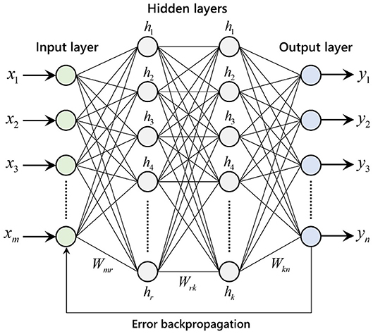
Figure 4. Architecture of multilayer artificial neural network with error backpropagation.

In ANNs, artificial neurons in consecutive layers are connected through a series of links. These links act as signal transmitters; resembling the synapses in a biological brain; and are allocated with adaptive weights which are calibrated during the training process using backpropagation algorithms. The training of BP networks typically consists of two stages; feedforward (or activation propagation) and error backpropagation. Figure 5 depicts the two stages for neuron j in a generic single layer BP ANN. During the feedforward stage, the input signal to the neuron (s_j) is computed as the sum of the weighted inputs and bias, as show in Figure 5, where W_ji is the weight of the link connecting neuron i of the preceding layer and neuron j, x_i is the input from neuron i of the previous layer, and b_j is the bias of the current neuron. The output signal y_j for the neuron j is then obtained by passing the input signal s_j through a non-linear transfer (activation) function. Common activation functions used in ANN for neurons in the hidden layer include the tangent sigmoid and the logarithmic sigmoid (Basheer and Hajmeer, 2000). In the case of multilayer ANNs, the output signal y_j is transmitted to the neurons of the following layer as an input signal.

FIGURE 5

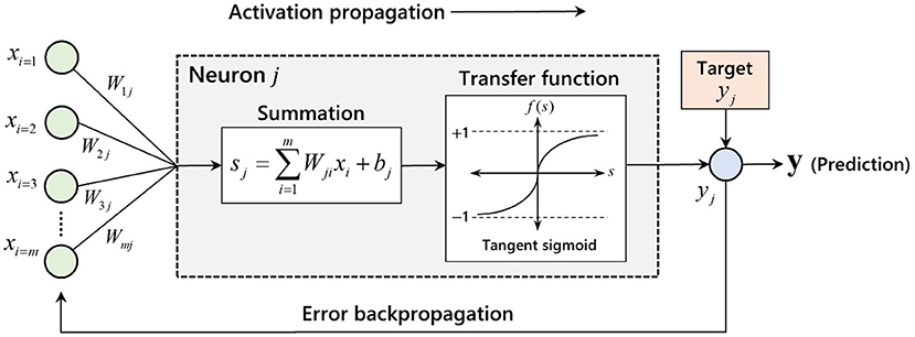
Figure 5. Feedforward (or activation propagation) and error backpropagation phases for neuron j.

At the end of the feedforward stage, the final output vector is compared to a target output; commonly through calculation of the mean squared error (MSE). The error is then back-propagated from the output layer to the input layer using a backpropagation training algorithm to adjust weights of the connecting links for minimization of the MSE. The error backpropagation stage continues until a convergence criteria is reached. The Levenberg–Marquardt (LM) backpropagation algorithm was selected in this study. The algorithm was designed to approach second-order training speed without having to compute the Hessian matrix, and has proven very efficient when training networks with up to a few hundred weights (Hagan and Menhaj, 1994); which is the case in the present study.

Predicting Mean, RMS, and Peak Roof Pressures Using ANN

Designing an ANN model requires the selection of multiple parameters; e.g., number of inputs and output, number of hidden layers, and the number of neurons in each layer. These parameters often have a strong influence in the performance and computational efficiency of the network. Currently, there are no general rules—and very few guidelines—for defining the optimum ANN architecture. Therefore, trial-and-error approaches are regularly employed to calibrate the network to achieve the best ANN structure for a particular problem (e.g., Bre et al., 2018). A common approach; which is adapted in this study; is to begin with a small number of neurons and progressively increase their number until achieving adequate training results and observing diminishing returns with further additional neurons.

In the current work, an ANN using a backpropagation training algorithm was employed to predict the distribution of mean, RMS, and peak pressure coefficients on the roof of a low-rise structure from the turbulence characteristics of the freestream. The ANN parameters are summarized in Table 2. The inputs to the ANN are the freestream turbulence intensity at eave height (I_{u, H}) and the normalized roof coordinates (x/H and y/H), while the ANN outputs are the mean (C_{p, mean}), RMS (C_{p, rms}), and peak (C_{p, peak}) pressure coefficients for all 152 roof taps (Figure 1) of each model. Peak values are estimated from a Fisher-Tippett Type I (Gumbel) distribution for a 78% probability of non-exceedance (Cook and Mayne, 1979). Although mean, RMS and peak C_p values were obtained from time series, the time-varying C_p signal is not an output of the ANN; i.e., statistical analysis of the pressure time series was performed prior to training the network. The hyperbolic tangent sigmoid function was selected as the transfer function for the hidden layers. The function can generate values in the range [−1, 1], and thus can accommodate for both positive (e.g., C_{p, rms}) and negative (e.g., C_{p, peak}) outputs. Linear transfer functions are used in the output layer. As previously mentioned, only the 45° wind direction is considered.

TABLE 2

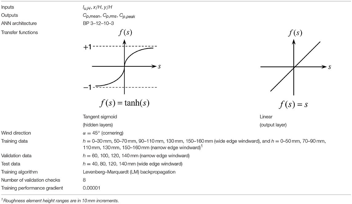
Table 2. Backpropagation ANN parameters for the 1:20, 1:30, and 1:50 building model.

For each model scale, the complete BLWT dataset was divided into subsets for training, validation, and testing of the ANN. The training data is used to adjust the weight and bias values of each neuron during ANN training (Figure 5). The validation data subset supervises the training process; without performing weight/bias adjustments; and can terminate the training process if the error (i.e., observed vs. predicted) of the validation subset increases repeatedly for a specified number of epochs (i.e., iterations). That is, the validation data serves as a stopping criteria during ANN training to improve generalization and avoid overfitting of the training data. Finally, the testing data subset is used to independently assess the predictive capabilities of the ANN model after training; i.e., the test data does not participate in the training process.

During training of the ANNs, multiple training initializations runs were performed due to the random nature of the weight and bias initialization functions in feedforward ANNs, which often produce variations in the training results. The termination criteria for the training process was chosen as the magnitude of the performance gradient (measured by the LM algorithm) and the number of validation checks. As training progresses, the performance gradient becomes significantly small. The training process terminates if the magnitude of the gradient falls below 0.00001. Further, the training was halted after eight validation checks. The number of validation checks represents the number of consecutive iterations that the validation performance fails to decrease.

Upwind terrains for both narrow and wide edge roughness element orientations were used for training the network; including the smoothest (h = 0 mm; i.e., flush floor) and roughest (h = 160 mm, wide edge) Terraformer configurations. These are listed in Table 2. The training data comprised nearly 76% of the upwind terrains. Four narrow edge element heights were chosen for validating the training data. Finally, roughness heights h = 40, 80, 120, and 140 mm for a wide edge windward orientation were selected to test the ANN.

Results

ANN Training Performance

Figure 6 depicts subplots of performance histories during ANN training for the 1:50, 1:30, and 1:20 datasets. The performance function was chosen as the combined MSE of the predicted (i.e., ANN) and observed (i.e., BLWT) mean, RMS, and peak C_p values. The training, validation, and test subsets each have predicted and observed values for the three C_p statistics. The LM backpropagation algorithm was employed to optimize (i.e., minimize) the MSE. At the end of the training process, the ANN for the 1:50 model achieved the lowest MSE from the three model scales, with a training performance of MSE = 0.021. Nevertheless, the three ANNs achieved satisfactory performance results.

FIGURE 6

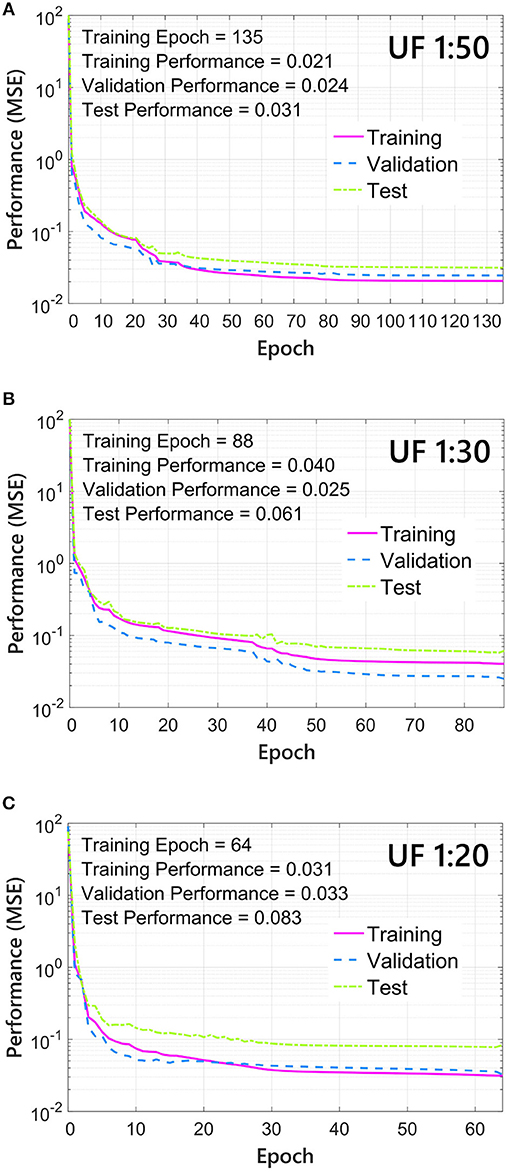
Figure 6. ANN backpropagation performance history for training, validation, and testing subsets: (A) 1:50, (B) 1:30, and (C) 1:20 building models.

Linear regression was performed on the ANN C_p outputs and BLWT data to assess the predictive power of the network. Figure 7 includes subplots of ANN outputs (i.e., predictions) of mean, RMS, and peak pressures plotted against observed BLWT data (i.e., target) for the three WERFL models. Each subplot in Figure 7 includes data points from all 152 roof taps and upwind terrains considered in the training, validation, and testing of the network. Error indices computed from least-squares linear fits of the data are also reported in the figure; i.e., root mean squared error (RMSE), mean absolute error (MAE), and coefficient of determination (R²); and are defined as

$\begin{array}{rc}RMSE=\sqrt{\frac{1}{n}{\displaystyle \sum _{i=1}^n}{(O_i-P_i)}^2}& (2)\end{array}$

$\begin{array}{rc}MAE=\frac{1}{n}{\displaystyle \sum _{i=1}^n}|O_i-P_i|& (3)\end{array}$

$\begin{array}{rc}{R}^2=1-\frac{{\displaystyle {\sum }_{i=1}^n}{(O_i-P_i)}^2}{{\displaystyle {\sum }_{i=1}^n}{(O_i-\overline{O})}^2}& (4)\end{array}$

where O_i is the observed BLWT data, P_i is the predicted ANN data, ō represents the mean value of the observed data and n represents the total number of data points in the subset. Values of RMSE and MAE near zero and R² close to unity indicate high predictive capability of the ANN model. Very good agreement is observed in mean, RMS, and peak pressures for all model scales and data subsets; i.e., training, validation, and test data. Particularly, the ANN model displays remarkable predictive capabilities on the test data; which is not used during the training process.

FIGURE 7

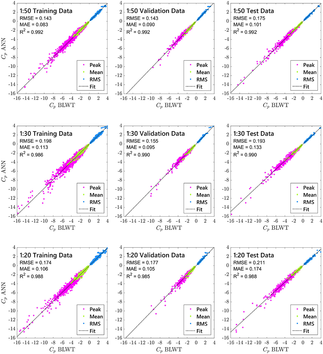
Figure 7. ANN regression plots showing the relationship between the outputs (C_p ANN) of the network and the targets (C_p BLWT) for the three WERFL building models.

Table 3 summarizes the test data error indices for the three C_p statistics individually. In the three model scales, peak pressure coefficients show higher values of MAE and RMSE when compared to RMS and mean C_p. For instance, MAE = 0.215 for the peak C_p data of the 1:50 model, while the RMS and mean MAE are 0.042 and 0.045, respectively. Further, MAE and RMSE of peak pressures appear to increase marginally for larger building models. The larger errors in peak C_p data can be attributed to the inherent uncertainties (i.e., variability) when estimating pressure extrema (Gavanski et al., 2016; Huang et al., 2017) which results in more spread in the data. This is reflected in Figure 7 where peak pressures (magenta markers) display a more scattered behavior than RMS and mean pressure data. Nevertheless, the R² of the peaks reported in Table 3 show very good results, and closely match R² values for mean and RMS pressures.

TABLE 3

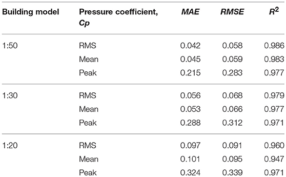
Table 3. Regression performance for ANN test data (h = 40, 80, 120, 140 mm; wide edge windward).

Predicting Roof Corner Pressures From Freestream Turbulence

Table 4 includes mean, RMS, and peak pressure coefficients predicted by the ANN model for three representative pressure taps located near the roof corner of the 1:50 model. Only ANN predictions from the test data are reported in the table; i.e., four upwind terrain configurations (see test data in Table 2). Roof tap 215 is located closest to the roof corner (x/H = 0.02, y/H = 0.04), while taps 301 and 314 are further away from the roof corner, but near roof edges (see Figure 1). These taps were strategically selected to evaluate the performance of the ANN model in extreme suction regions resulting from a cornering wind direction. In general, ANN results show remarkable predictive power for the 1:50 model. For example, the largest errors reported for tap 215 were −3.7, +4.1, and +14.4% for the mean, RMS, and peak pressures, respectively. The smallest error in the peak was −0.7% corresponding to tap 314 for a freestream turbulence of I_{u, H} = 26.9% (h = 140 mm). The distribution of peak pressures on the 1:50 model for this upstream condition is illustrated in Figure 8 for both the BLWT data and ANN model.

TABLE 4

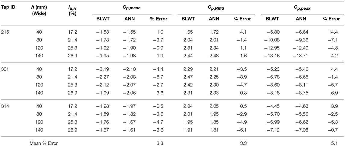
Table 4. Prediction of mean, RMS, and peak pressures for taps 215, 301, and 314 on the 1:50 building model.

FIGURE 8

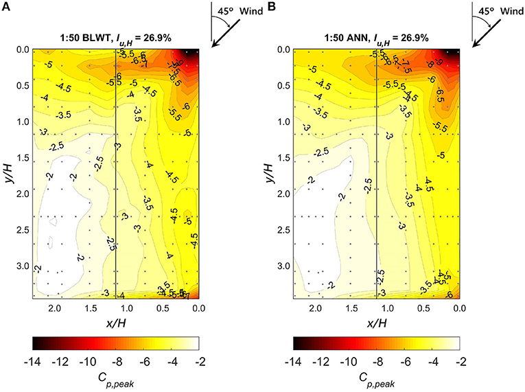
Figure 8. Prediction of peak pressure coefficients (C_{p, peak}) for the 1:50 WERFL model and a freestream turbulence intensity of 26.9% at eave height: (A) BLWT experimental data and (B) ANN prediction.

ANN C_p predictions of roof corner taps 215, 301, and 316 for the 1:30 model (see Figure 1) are listed in Table 5. For the most part, reasonably good agreement is found between the ANN model and BLWT data. Particularly, the ANN model was highly proficient in predicting the mean, RMS, and peak pressures for taps 215 and 314, where the highest errors in C_{p, mean} were −9.7 and −5.4%, respectively. However, noticeable discrepancies are evident in the mean and RMS pressures for tap 301, where the ANN model consistently underestimated the BLWT data (i.e., negative % errors). This was also observed on the 1:50 model; although to a lesser extent. These discrepancies are noticeable in Figure 9; i.e., “hot spots” near the roof edge of the short building dimension. Yet, the distribution of mean pressures predicted by the ANN model closely resembles the wind tunnel data. Moreover, the ANN model shows good predictive performance of the peaks, where errors between the ANN model and BLWT data were <10% in most cases.

TABLE 5

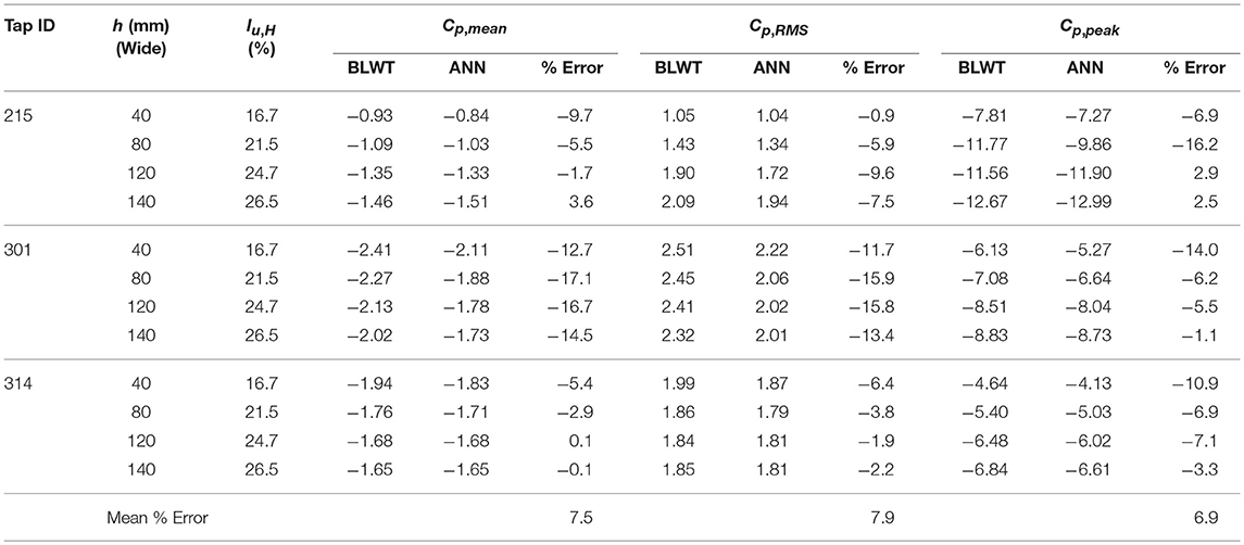
Table 5. Prediction of mean, RMS, and peak pressures for taps 215, 301, and 314 on the 1:30 building model.

FIGURE 9

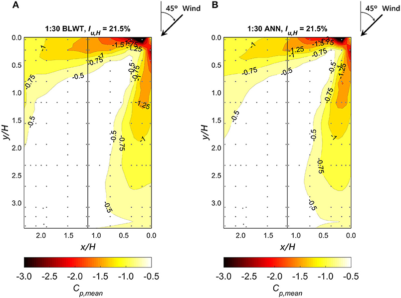
Figure 9. Prediction of mean pressure coefficients (C_{p, mean}) for the 1:30 WERFL model and a freestream turbulence intensity of 21.5% at eave height: (A) BLWT experimental data and (B) ANN prediction.

Table 6 summarizes ANN C_p results obtained for the 1:20 model at the three roof tap locations considered in Tables 4, 5. In general, the ANN model demonstrates adequate predictive performance of peak pressures for the three corner taps, where absolute errors between 1.2 and 21.9% were found. However, similar to the 1:50 and 1:30 models, lower mean and RMS pressures are predicted by the ANN model at tap 301 compared to the BLWT data. This is observed for the four upwind terrain cases. Additionally, ANN predictions of the mean C_p for tap 314 display noticeable deviations from the BLWT data. Figure 10 presents contour maps of observed and predicted (i.e., ANN) RMS pressures on the roof of the 1:20 model for I_{u, H} = 22.1% (h = 8 mm; wide). This upwind terrain configuration corresponds to the largest errors in both mean and RMS in the 1:20 model. The pressure maps illustrate how the ANN underestimates the intensity of the RMS pressures. Nevertheless, the errors in the mean and RMS pressures did not seem to affect the prediction of the peaks, where more than half of the values reported in Table 6 were <3.8% of the BLWT data. Of the three model scales, the ANN performed the best on the 1:50 dataset, while the 1:20 produced the largest discrepancies between the model and BLWT data.

TABLE 6

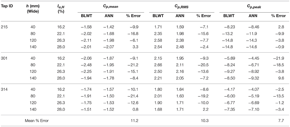
Table 6. Prediction of mean, RMS, and peak pressures for taps 215, 301, and 314 on the 1:20 building model.

FIGURE 10

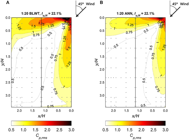
Figure 10. Prediction of RMS pressure coefficients (C_{p, rms}) for the 1:20 WERFL model and a freestream turbulence intensity of 22.1% at eave height: (A) BLWT experimental data and (B) ANN prediction.

Turbulence Effects on Area-Averaged Peak Pressures

Figure 11 includes subplots of area-averaged peak pressures acting on the roof corner as a function of freestream turbulence intensity at eave height (I_{u, H}). The area-averaged pressures were computed from peak C_p estimates of taps 215, 216, 301, 316, 315, and 314 located near the roof corner of the three WERFL models (see Figure 1). The six taps cover a normalized corner roof area A/H² of 0.15, where H is the eave height of the model; ~2.35 m² in full-scale. In Figure 11, the red markers represent BLWT data from the 33 upwind terrain configurations, while the continuous black line is the ANN analytical (predictive) model. Peak pressure estimates were calculated from Gumbel distribution for a 78% probability of non-exceedance.

FIGURE 11

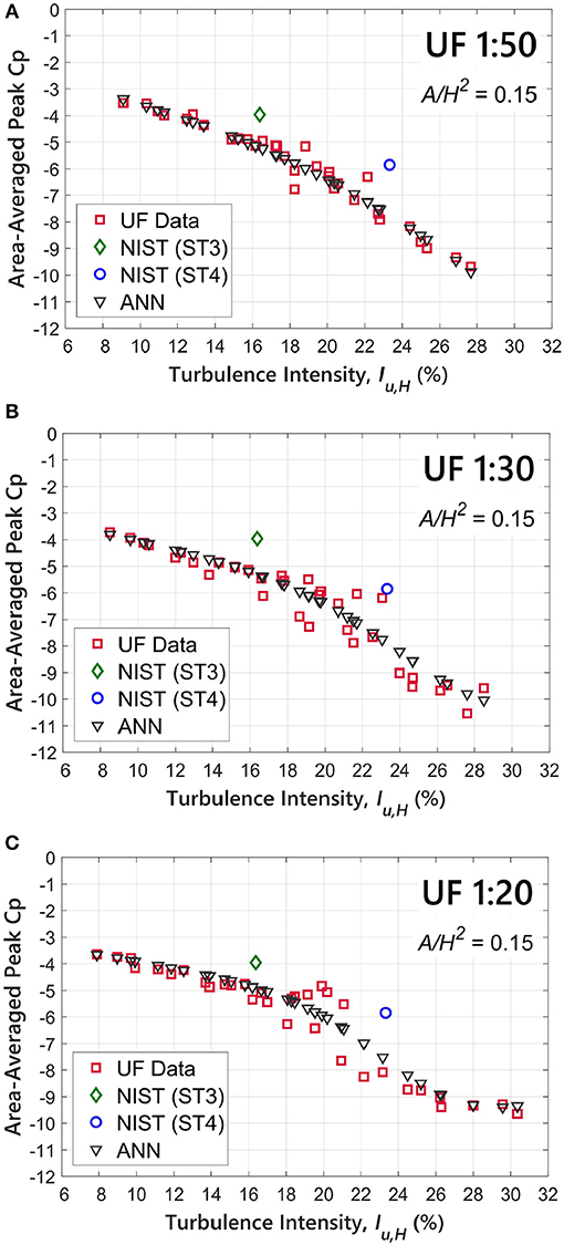
Figure 11. Area-averaged peak pressures from six corner roof taps (Tap IDs 215, 216, 301, 314, 315, and 316) as a function of freestream turbulence: (A) 1:50, (B) 1:30, and (C) 1:20.

Area-average pressures for the three WERFL models display similar trends of increasing peak suction with freestream turbulence. For the smoothest upwind case (I_{u, H} ~8%), the three scales display peak pressures of approximately −3. Further, little scatter is observed for turbulence levels ranging from 8 to 18%. In this range, the ANN model is able to closely follow the monotonic trend in the data. However, for I_{u, H} exceeding 18%, the scattering in the UF data becomes more pronounced. During the ANN training process, the network parameters were carefully calibrated to avoid overfitting of data subsets with significant scatter (i.e., variability); e.g., peak pressure data associated with highly turbulent approach flow conditions. This is particularly evident in the 1:30 and 1:20 building models. This resulted in improved generalization of ANN model for the roughest upwind cases.

The subplots in Figure 11 also include area-averaged peak estimates computed from tests ST3 and ST4 of the NIST database. The turbulence intensity for the two experiments were derived from the ESDU (1983) model based on full-scale roughness lengths of z₀ = 0.01 and 0.087 m and a height z = 3.96 m above ground level. This resulted in turbulence levels of 16.4 and 23.3% for ST3 and ST4, respectively. Area-averaged peak values for test ST3 (diamond green marker) show reasonably good agreement with the UF data when matching the turbulence levels at eave height, although NIST results displayed slightly lower peak (area-averaged) suction values. Conversely, the averaged peak pressure for test ST4 (square blue marker) shows noticeable discrepancies when compared to the UF data for similar I_{u, H}. The discrepancy could be, in part, ascribed to uncertainties in the turbulent characteristics of the approach flow during pressure testing; i.e., surface pressures and approach flow conditions near the model are usually not measured simultaneously. For example, Figure 11 reveals how a slight reduction in I_{u, H} (e.g., 2%) can cause the NIST data to fall in line with the UF observations. This sheds light regarding the sensitivity of peak pressures to the turbulent flow conditions of the freestream.

Discussion

In general, the results suggest that the ANN models can accurately predict mean, peak, and fluctuating (i.e., RMS) pressures within the range of turbulent flow conditions considered. However, in some cases, considerable errors exist between experimental BLWT data and ANN predictions; particularly for the larger building models (e.g., 1:20). Discrepancies between BLWT data and the ANN model appear to increase with building model scale for taps near roof corners. For instance, the largest errors reported for mean pressure coefficients correspond to the 1:20 model (see Table 6). Peak and RMS C_p values also show relatively large errors for the largest building model. While it is evident that the turbulence intensity of the freestream near the model height is a key factor for predicting peak surface pressures, previous studies (e.g., Tieleman, 1992; Saathoff and Melbourne, 1997) have shown that the turbulence scales of the incident flow also play an important role in the development of extreme pressures, particularly in the mechanisms of transition within the separated shear layer (e.g., Lander et al., 2018).

Early experimental work presented in Gartshore (1973) and Laneville (1975) has demonstrated the effect of the small-scale turbulence on the flow structure near the separated shear layer. These small-scale eddies; approximately of the same order as the thickness of the shear layer; predominantly control the roll-up in flow separation regions. The level of small-scale turbulence is typically quantified by the Melbourne parameter (1979), defined as the normalized spectral density of the longitudinal velocity fluctuations evaluated at a wavelength (nH/U) corresponding to 1/10 of the characteristic dimension (e.g., eave height, H) of the bluff body. Further, it has been shown that large-scale turbulence; represented by the integral length scale $L_u^x$; can also influence the development and duration of extreme pressure events (Tieleman, 2003). For instance, Saathoff and Melbourne (1997) reported a noticeable increase in peak pressures; measured on a blunt flat plate; with increasing $L_u^x$ for the same turbulence intensity, although the turbulence levels were in relatively smoother flows (I_{u, H} ~8 and 12%). These authors argue that large-scale turbulent eddies are less frequent and thus permit shear layer vortices to further develop and strengthen, which results in higher surface pressures near flow separated regions. Nevertheless, further research is needed to better understand (and more accurately quantify) the effect of small- and large-scale turbulence features in the freestream flow and their influence on peak pressures; particularly for bluff-bodies immersed in highly turbulent boundary layers. It can be inferred from Figure 11 that the largest discrepancies between the BLWT data and ANN for the 1:30 and 1:20 models are generally found in BLWT experiments where the model is immersed in more turbulent boundary layer flows (e.g., I_{u, H} > 18%). These observations are consistent with previous BLWT studies (Fritz et al., 2008) which have shown significant variability in peak pressures near roof corners when simulating rougher (i.e., suburban) upwind terrain conditions in the wind tunnel.

Results from the three building models also suggest a clear dependence of the building model size on the performance of the neural network, where ANN predictions generally display larger discrepancies in peak pressures with increasing model scale. This trend could be, in part, due to Reynolds number effects in the BLWT; e.g., the Re for the 1:20 model is ~2.5 times greater than the 1:50 model. Previous work (e.g., Lim et al., 2007) has demonstrated the Re-dependence (that can persist well-beyond Re > 2 × 10⁴) when quantifying peak suction pressures on sharp-edged bluff bodies oriented at 45° to the approach flow; which is the wind direction considered in this study. This wind orientation promotes the development of strong (and relatively steady) “delta-wing type” conical vortices that originate at roof corners and extend along line inclines of ~11–14° relative to roof edges, where smaller angles are associated with larger Re numbers (Tryggeson and Lyberg, 2010). The structure of conical vortices has been shown to strongly affect Re, which partly explains the well-known mismatch between measured peak pressures at model and full-scale under corner roof vortices (Cochran, 1992). Consequently, these disparities should be accounted for when deriving full-scale pressure data from BLWT experiments. Nonetheless, further work must be conducted to properly correct these discrepancies.

Conclusions

A feed-forward multilayer ANN using a backpropagation (BP) training algorithm is developed to predict the mean, RMS, and peak pressures on the roof of three geometrically scaled low-rise building models for a wide-range of upwind approach flow conditions. A large dataset of BLWT experimental data was utilized to train, validate, and test the network. The dataset consists of pressure data collected on the surface of three low-rise building models immerse in 33 unique boundary layer flows. In general, results indicate that the ANN model can accurately predict mean, RMS, and peak pressure coefficients on the roof of a low-rise structure given the freestream turbulence intensity at eave height and the normalized plan roof coordinates. Predicted ANN peak pressure coefficients for a series of pressure taps located near the roof corner were, on average, within 5.1, 6.9, and 7.7% of observed BLWT data for the 1:50, 1:30, and 1:20 model scales, respectively. The network also displayed reasonably good agreement between predicted ANN mean and RMS pressure coefficients and BLWT data. Further, the ANN was also successful in generating reliable functional relationships to associate area-averaged peak pressures near the roof corner to the turbulence characteristics of the freestream. These relationships similar trends for the three WERFL building models.

While the present work centers on the prediction of peak surface pressures from the freestream turbulence intensity near the model height, it is well-established that other flow parameters can influence the extreme pressure distribution, particularly in the separated shear layer. Both small and large turbulence scales in the freestream can affect the magnitude and duration of peak pressure events. These turbulent scale properties could potentially be introduced into the ANN model as input parameters (in addition to I_{u, H}), where small turbulence scales could be quantified by the Melbourne parameter, while the integral length scale ($L_u^x$) can be utilized to estimate the size of large-scale turbulent eddies in the incident flow. Nonetheless, a better understanding of these parameters and their effect on the flow field around flow separated regions is still needed to more accurately predict peak pressures.

In summary, the development of new predictive tools for quantifying peak wind loading on civil infrastructure is essential for improving the numerical accuracy of computational modeling (e.g., CFD) and steadily reducing our dependence on experimental testing. For instance, ANNs can be used to expand existing aerodynamic databases and help cover a wide range of possible experimental configurations. Further, ANNs can enhance the efficiency of newly developed cyber-physical methods (e.g., Whiteman et al., 2018) for investigating and optimizing the performance of civil infrastructure systems under wind hazards. Future work will further expand the capabilities of the current ANN model by incorporating additional input parameters, such as wind direction, roof slope, and building aspect ratio (Chen et al., 2003; e.g., Bre et al., 2018). Additionally, the predictive power of the neural network can be further enhanced through simulation of more realistic upwind terrain conditions. This can be achieved experimentally through the generation of random fields of roughness elements to recreate real-world heterogeneous terrain conditions.

Author Contributions

PF-C performed the data analysis, prepared the figures and tables, and drafted the paper with input from FM and BP. FM and BP provided valuable guidance in developing the paper in addition to revising the data analysis procedures.

Funding

Experimental support for this research was provided by the National Science Foundation through the NSF Natural Hazards Engineering Research Infrastructure (NHERI, CMMI-1520843) Experimental Facility at the University of Florida (UF). The development and drafting of the paper was supported by NSF under Grant No. 1636039.

Conflict of Interest Statement

The authors declare that the research was conducted in the absence of any commercial or financial relationships that could be construed as a potential conflict of interest.

Acknowledgments

The authors wish to recognize the Powell Structures and Materials Laboratory staff, with special thanks to Jon Sinnreich, Steve Schein, Eric Agostinelli, Kevin Stultz, and Shelby Brothers for their contribution in wind tunnel testing. Any opinions, findings, and conclusions or recommendations expressed in this paper are those of the authors and do not necessarily reflect the views of the sponsors, partners, and contributors.

References

Akon, A. F., and Kopp, G. A. (2016). Mean pressure distributions and reattachment lengths for roof-separation bubbles on low-rise buildings. J. Wind Eng. Ind. Aerodyn. 155, 115–125. doi: 10.1016/j.jweia.2016.05.008

CrossRef Full Text | Google Scholar

Basheer, I. A., and Hajmeer, M. (2000). Artificial neural networks: fundamentals, computing, design, and application. J. Microbiol. Methods 43, 3–31. doi: 10.1016/S0167-7012(00)00201-3

PubMed Abstract | CrossRef Full Text | Google Scholar

Bre, F., Gimenez, J. M., and Fachinotti, V. D. (2018). Prediction of wind pressure coefficients on building surfaces using artificial neural networks. Energy Build. 158, 1429–1441. doi: 10.1016/j.enbuild.2017.11.045

CrossRef Full Text | Google Scholar

Bruno, L., Salvetti, M. V., and Ricciardelli, F. (2014). Benchmark on the aerodynamics of a rectangular 5: 1 cylinder: an overview after the first four years of activity. J. Wind Eng. Ind. Aerodyn. 126, 87–106. doi: 10.1016/j.jweia.2014.01.005

CrossRef Full Text | Google Scholar

Chen, Y., Kopp, G. A., and Surry, D. (2003). Prediction of pressure coefficients on roofs of low buildings using artificial neural networks. J. Wind Eng. Ind. Aerodyn. 91, 423–441. doi: 10.1016/S0167-6105(02)00381-1

CrossRef Full Text | Google Scholar

Cochran, L. S. (1992). Wind-Tunnel Modelling of Low-Rise Structures. Ph.D. Thesis, Civil Engineering, Colorado State University, CO.

Cook, N. J., and Mayne, J. R. (1979). A novel working approach to the assessment of wind loads for equivalent static design. J. Wind Eng. Ind. Aerodyn. 4, 149–164. doi: 10.1016/0167-6105(79)90043-6

CrossRef Full Text | Google Scholar

Dongmei, H., Shiqing, H., Xuhui, H., and Xue, Z. (2017). Prediction of wind loads on high-rise building using a BP neural network combined with POD. J. Wind Eng. Ind. Aerodyn. 170, 1–17. doi: 10.1016/j.jweia.2017.07.021

CrossRef Full Text | Google Scholar

ESDU (1983). Strong Winds in the Atmospheric Boundary Layer, Part 2: Discrete Gust Speeds, Engineering Sciences Data Unit, Itm. No. 83045, London, UK.

Fernández-Cabán, P. L., and Masters, F. J. (2017). Near surface wind longitudinal velocity positively skews with increasing aerodynamic roughness length. J. Wind Eng. Ind. Aerodyn. 169, 94–105. doi: 10.1016/j.jweia.2017.06.007

CrossRef Full Text | Google Scholar

Fernández-Cabán, P. L., and Masters, F. J. (2018). Upwind Terrain Effects on Low-Rise Building Pressure Loading Observed in the Boundary Layer Wind Tunnel. DesignSafe-CI, Dataset. doi: 10.17603/DS2W670

CrossRef Full Text

Fernández-Cabán, P. L., and Masters, F. J. (2018). Effects of freestream turbulence on the pressure acting on a low-rise building roof in the separated flow region. Front. Built Environ. 4:17. doi: 10.3389/fbuil.2018.00017

CrossRef Full Text | Google Scholar

Franke, R. (1982). Scattered data interpolation: tests of some methods. Math. Comput. 38, 181–200.

Google Scholar

Fritz, W. P., Bienkiewicz, B., Cui, B., Flamand, O., Ho, T. C., Kikitsu, H., et al. (2008). International comparison of wind tunnel estimates of wind effects on low-rise buildings: test-related uncertainties. J. Struct. Eng. 134, 1887–1890. doi: 10.1061/(ASCE)0733-9445(2008)134:12(1887)

CrossRef Full Text | Google Scholar

Fu, J. Y., Li, Q. S., and Xie, Z. N. (2006). Prediction of wind loads on a large flat roof using fuzzy neural networks. Eng. Struct. 28, 153–161. doi: 10.1016/j.engstruct.2005.08.006

CrossRef Full Text | Google Scholar

Gartshore, I. S. (1973). The Effects of Free Stream Turbulance on the Drag of Rectangular Two-dimentional Prism. University of Western Ontario, Faculty of Engineering Science, Boundary Layer Wind Tunnel Laboratory.

Gartshore, I. S. (1984). Some effects of upstream turbulence on the unsteady lift forces imposed on prismatic two dimensional bodies. J. Fluids Eng. 106, 418–424. doi: 10.1115/1.3243140

CrossRef Full Text | Google Scholar

Gavalda, X., Ferrer-Gener, J., Kopp, G. A., and Giralt, F. (2011). Interpolation of pressure coefficients for low-rise buildings of different plan dimensions and roof slopes using artificial neural networks. J. Wind Eng. Ind. Aerodyn. 99, 658–664. doi: 10.1016/j.jweia.2011.02.008

CrossRef Full Text | Google Scholar

Gavanski, E., Gurley, K. R., and Kopp, G. A. (2016). Uncertainties in the estimation of local peak pressures on low-rise buildings by using the Gumbel distribution fitting approach. J. Struct. Eng. 142:04016106. doi: 10.1061/(ASCE)ST.1943-541X.0001556

CrossRef Full Text | Google Scholar

Ghosh, J., and Shin, Y. (1992). Efficient higher-order neural networks for classification and function approximation. Int. J. Neural Syst. 3, 323–350. doi: 10.1142/S0129065792000255

CrossRef Full Text | Google Scholar

Hagan, M. T., and Menhaj, M. B. (1994). Training feedforward networks with the Marquardt algorithm. IEEE Trans. Neural Netw. 5, 989–993. doi: 10.1109/72.329697

PubMed Abstract | CrossRef Full Text | Google Scholar

Haykin, S. (1994). Neural Networks: A Comprehensive Foundation. Upper Saddle River, NJ: Prentice Hall PTR.

Google Scholar

Hillier, R., and Cherry, N. J. (1981). The effects of stream turbulence on separation bubbles. J. Wind Eng. Ind. Aerodyn. 8, 49–58. doi: 10.1016/0167-6105(81)90007-6

CrossRef Full Text | Google Scholar

Ho, T. C. E., Surry, D., and Morrish, D. P. (2003). NIST/TTU Cooperative Agreement–Windstorm Mitigation Initiative: Wind Tunnel Experiments on Generic Low Buildings. The Boundary Layer Wind Tunnel Laboratory, The University of Western Ontario, London, Ontario, Canada.

Huang, G., Ji, X., Zheng, H., Luo, Y., Peng, X., and Yang, Q. (2017). Uncertainty of peak value of non-Gaussian wind load effect: analytical approach. J. Eng. Mech. 144:04017172. doi: 10.1061/(ASCE)EM.1943-7889.0001402

CrossRef Full Text | Google Scholar

Irwin, H. P. A. H., Cooper, K. R., and Girard, R. (1979). Correction of distortion effects caused by tubing systems in measurements of fluctuating pressures. J. Wind Eng. Ind. Aerodyn. 5, 93–107. doi: 10.1016/0167-6105(79)90026-6

CrossRef Full Text | Google Scholar

Lander, D. C., Moore, D. M., Letchford, C. W., and Amitay, M. (2018). Scaling of square-prism shear layers. J. Fluid Mech. 849, 1096–1119. doi: 10.1017/jfm.2018.443

CrossRef Full Text | Google Scholar

Laneville, A. (1975). “An explanation of some effects of turbulence on bluff bodies,” in Proc. Fourth International Conference on Wind Effects on Building and Structures (Heathrow).

Google Scholar

Levitan, M. L., and Mehta, K. C. (1992a). Texas Tech field experiments for wind loads part 1: building and pressure measuring system. J. Wind Eng. Ind. Aerodyn. 43, 1565–1576. doi: 10.1016/0167-6105(92)90372-H

CrossRef Full Text | Google Scholar

Levitan, M. L., and Mehta, K. C. (1992b). Texas Tech field experiments for wind loads part II: meteorological instrumentation and terrain parameters. J. Wind Eng. Ind. Aerodyn. 43, 1577–1588. doi: 10.1016/0167-6105(92)90373-I

CrossRef Full Text | Google Scholar

Lim, H. C., Castro, I. P., and Hoxey, R. P. (2007). Bluff bodies in deep turbulent boundary layers: Reynolds-number issues. J. Fluid Mech. 571, 97–118. doi: 10.1017/S0022112006003223

CrossRef Full Text | Google Scholar

Melbourne, W. H. (1979). “Turbulence effects on maximum surface pressures, a mechanism and possibility of reduction,” in Proc. 5th Int. Conf. on Wind Engineering (Fort Collins, CO: Pergamon Press), 541–552.

Google Scholar

Nasrabadi, N. M. (2007). Pattern recognition and machine learning. J. Electron. Imaging 16:049901. doi: 10.1117/1.2819119

CrossRef Full Text | Google Scholar

Pemberton, R. (2010). An Overview of Dynamic Pressure Measurement Considerations. Liberty Lake, WA: Scanivalve Corporation.

Google Scholar

Ricci, M., Patruno, L., and de Miranda, S. (2017). Wind loads and structural response: benchmarking LES on a low-rise building. Eng. Struct. 144, 26–42. doi: 10.1016/j.engstruct.2017.04.027

CrossRef Full Text | Google Scholar

Rumelhart, D. E., Hinton, G. E., and Williams, R. J. (1986). Learning representations by back-propagating errors. Nature 323:533. doi: 10.1038/323533a0

CrossRef Full Text | Google Scholar

Saathoff, P. J., and Melbourne, W. H. (1997). Effects of free-stream turbulence on surface pressure fluctuations in a separation bubble. J. Fluid Mech. 337, 1–24. doi: 10.1017/S0022112096004594

CrossRef Full Text | Google Scholar

Scanivalve. (2016). ZOC33 Miniature Pressure Scanner. Available online at: http://scanivalve.com/products/pressure-measurement/miniature-analog-pressure-scanners/zoc33-miniature-pressure-scanner/ (Accessed March 13, 2018).

St. Pierre, L. S., Kopp, G. A., Surry, D., and Ho, T. C. E. (2005). The UWO contribution to the NIST aerodynamic database for wind loads on low buildings: part 2. Comparison of data with wind load provisions. J. Wind Eng. Ind. Aerodyn. 93, 31–59. doi: 10.1016/j.jweia.2004.07.007

CrossRef Full Text | Google Scholar

Tieleman, H. W. (1992). Problems associated with flow modelling procedures for low-rise structures. J. Wind Eng. Ind. Aerodyn. 42, 923–934. doi: 10.1016/0167-6105(92)90099-V

CrossRef Full Text | Google Scholar

Tieleman, H. W. (2003). Wind tunnel simulation of wind loading on low-rise structures: a review. J. Wind Eng. Ind. Aerodyn. 91, 1627–1649. doi: 10.1016/j.jweia.2003.09.021

CrossRef Full Text | Google Scholar

Tieleman, H. W., Reinhold, T. A., and Marshall, R. D. (1978). On the wind-tunnel simulation of the atmospheric surface layer for the study of wind loads on low-rise buildings. J. Wind Eng. Ind. Aerodyn. 3, 21–38. doi: 10.1016/0167-6105(78)90026-0

CrossRef Full Text | Google Scholar

Tryggeson, H., and Lyberg, M. D. (2010). Stationary vortices attached to flat roofs. J. Wind Eng. Ind. Aerodyn. 98, 47–54. doi: 10.1016/j.jweia.2009.09.001

CrossRef Full Text | Google Scholar

Turkkan, N., and Srivastava, N. K. (1995). Prediction of wind load distribution for air-supported structures using neural networks. Can. J. Civil Eng. 22, 453–461. doi: 10.1139/l95-053

CrossRef Full Text | Google Scholar

Whiteman, M. L., Fernández-Cabán, P. L., Phillips, B. M., Masters, F. J., Bridge, J. A., and Davis, J. R. (2018). Multi-objective optimal design of a building envelope and structural system using cyber-physical modeling in a wind tunnel. Front. Built Environ. 4:13. doi: 10.3389/fbuil.2018.00013

CrossRef Full Text | Google Scholar

Zhang, A., and Zhang, L. (2004). RBF neural networks for the prediction of building interference effects. Comput. Struct. 82, 2333–2339. doi: 10.1016/j.compstruc.2004.05.014

CrossRef Full Text | Google Scholar