An Iterative Parallel Solver in GPU Applied to Frequency Domain Linear Water Wave Problems by the Boundary Element Method

1. Introduction

The Boundary Element Method (BEM) is a numerical technique to obtain approximated solutions of partial differential equations. The origins of the method comes from Finite Element Method (FEM) ideas in the 1970s. The paper by Cheng and Cheng (2005) shows the previous works and the initials of the BEM. The birth date of the technique is considered in 1963, with the first paper by Jaswon and Porter (1963). The first BEM conference was held at Southampton University in 1978, and the first book was published in the same year, by Brebbia (1978). With refference to three-dimensional boundary value problem, the basic idea of the BEM is the use of boundary integral equations for primary variables at internal points (e.g., displacements, or potentials), and its extension to boundary points after a limit-to-the-boundary process. The integrals are interpreted in the sense of the Cauchy Principal Values (primary variables) or the Hadamard Finite Parte (derived variables). To solve a boundary value problem, a mesh is defined at the boundary, and the integral equation is used at collocation points. A fully-populated coefficient system matrix is obtained. Comparing to the FEM, the BEM is a boundary method, in the sense that the numerical discretization is carried out at reduced spatial dimension (e.g., in three-dimensional problems, a mesh is required only at the surfaces). This reduced dimension leads to smaller linear systems, less computer memory requirements, and more efficient computation.

The BEM is particularly well suited in wave problems due to mesh reduction and the natural treatment of radiation boundary conditions. Thus, it is an efficient competitor of some particuar techniques, such as the partition of unity method in diffraction and refraction problems (Ortiz and Sánchez, 2001; Ortiz, 2004) in the Finite Element Method.

The classical book by Brebbia and Dominguez (1996) explain the basic BEM theory and applications for potential and solid mechanics. The book by Bonnet Bonnet (1999) is a recent reference, with applications to solid and fluid mechanics. In the specific context of fluid mechanics, Hess (1990) introduced the panel method, which is equivalent to BEM techniques; the book by Brebbia and Partridge (1992) is focused on particular BEM topics for fluid mechanics.

Besides the inherent advantages, the BEM shows some disadvantages for systems with large number of degrees of freedom. In the standard BEM, the system matrix is fully populated, without symmetry or sparsity structures. This causes that the main bottleneck in computing times comes from the solver task. The use of acceleration iterative solvers, popular in FEM (e.g., the conjugate gradient) can not be used in BEM. For large system of equations this problem is crucial and makes the standard BEM not competitive with respect to other domain techniques, such as the Finite Element Method. This is particularly notorious in wave problems in the frequency domain, where the system matrix is complex-valued and fine meshes with large number of degrees of freedom are required.

In the BEM literature several acceleration techniques have been developed for large systems. The review paper by Liu et al. (2012) shows historical aspects and recent advances in acceleration methods for the BEM. A first approach consists on the multipole expansion of the Green functions, with an iterative solver. This is known as the Fast Multipole Method (FMM). The FMM has been regarded as one of the top 10 algorithms in scientific computing and has progressed very significantly. It was first introduced by Rokhlin (1985) in potential problems. The tutorial by Liu and Nishimura (2006) explain the basic algorithm and implementation details. The FMM has been extended to other fields: in elastostatic, Liu (2008) develops the algorithm for hipersingular 2D boundary integral equations in multidomain problems; Djojodihardjo (2010) considers the use of the FMM in FEM-BEM acoustic-structural interaction; in 3D time-harmonic elastodynamics, Chaillat and Bonnet (2013) review the basic developments in FMM; in electromagnetism, the book by Gumerov and Duraiswami (2005) shows a detailed exposition of the FMM applied to the solution of the general three-dimensional Helmholtz equation. The book by Liu (2009) covers the basic FMM algorithms for potential, elastostatics, Stokes flow and acoustic waves. Fortran codes are included.

When the FMM is implemented in a code based on the sequential use of the Central Processing Unit (CPU) for a system with N unknowns, the computing times is considerably reduced, with times ${O}(N^{1.5})$, or even ${O}(N{log}_{2}N)$ with a multilevel approach (see López-Portugués et al., 2012).

The implementation of the FMM algorithm requires a strong redesign of an existing code: a new hierarchical mesh of reference points must be created, and the multipole expansion modifies the way in which the system matrices are computed. The method is also dependent on the kind of multipole expansion of the Green function. The multipole expansion is not unique, and it is not available for any Green function. As a consequence, the FMM is not a general method. In the literature there have been developed different strategies to accelerate a BEM code, independent on the Green function. Such techniques can be classified into two groups: the pFFT (pre-corrected Fast Fourier Transformation) and the ACA (Adaptive Cross Approximation).

The pFFT method was proposed in 1997 by Phillips (1997); Phillips and White (1997), in the context of potential problems, with Laplace and Helmhotz equations as the governing equation. It has been extended to other fields in the BEM: Stokes equation, linear elasticity, coupled electrostatic and elasticity, Poisson, dynamics and quasi-linear equations (described in Liu et al., 2012). In the pFFT the algorithm does not depend on the Green function, and its implementation is easy. The computing time in a sequential CPU implementation are O(N)+O(N_glog₂N_g), with N_g the number of nodes of an auxiliary mesh, which is required by the method.

The ACA method (Lu et al., 2004; Benedetti et al., 2008) is in the context of methods in which the improvement comes from the acceleration of the solver, with the use of hierarchical matrices, introduced by Hackbusch (1999). The system matrix is approximate by a low-rank expansion.

The Generalized Minimum Residual Method (GMRES) is an iterative solver for the general use in the BEM. It was introduced by Saad and Shultz (1986). It is based on Krylov subspaces approximations. The main attraction of the GMRES comes from its direct use with fully-populated matrices, typical in the collocation BEM. Its use is widely extended, as a direct solver or to accelerate other fast methods, as FMM or AKA. Leung and Walker (1997) developed a combined GMRES with Dual Compensation method in 3D elastostatics. In multipole BEM, Margonari and Bonnet (2005) developed a combined BEM-FEM method in 3D elastostatics; the GMRES is used to solve the linear system of equations, and the FMM to accelerate the matrix-vector multiplications. In AKA, Brancati et al. (2009) combine the use of hierarchical matrices with GMRES in acoustics.

In comparison with the FMM, pFFT, or ACA, the main advantage of the GMRES is its use as a direct solver; it does not require modifications of an existing BEM code respect to the collocation schema and generation of the system matrices. The computational cost of the GMRES is ${O}(N^2)$.

Recent advances in computing hardware have extended the implementation of parallelization to improve the solver performances. The parallelizaction can be carried out in multi-core CPU (Central Processing Unit) systems. In addition, the use of the Graphics Processing Unit (GPU) for massive parallelization is extending nowadays. Its first use comes from the Graphics processors developed by NVIDIA, and the computing languaje CUDA (Computer Unified Device Architecture) Sanders and Kandrot (2010). Thus, a new computing paradigm has been developed for numerical analysis, based on heterogeneous massive parallel computation (Kirk and Hwu, 2012). This paradigm requires a new global vision of codes, by splitting the global tasks in blocks which are best suited to be executed in the CPU, and blocks which are best suited to be executed in massive parallel GPU processors.

The use of the GPU to accelerate the BEM is a recent trend since 2009. Hamada and Takahashi (2009) show the use of the GPU in the collocation stage, in acoustic wave problems governed by the Helmholtz equation. Wang et al. (2011), used the GPU to accelerate both the collocation task and the solver stage, in elastostatics problems, with the Dual-Compensation GMRES solver. Wang et al. (2013) used the GPU with the FMM to develop an adaptive solver in 3D elasticity. In the context of the standard collocation mehtod, the use of the GPU to perform the global matrix assembly and the LU factorization is reported in the work by D'Azevedo and Nintcheu Fata (2012).

In the context fluid dynamics and meshless methods, Kelly et al. (2014) explore a GPU implementation of an incompressible Navier-Stokes code based on a Radial-Basis Function Collocation Meshless Method for two-fluid flows. For compressive flows, Ma et al. (2014) show a GPU implementation.

The acceleration of the GMRES in GPU is explored by Li and Saad (2013) for sparse matrices; in this paper, the BEM is not considered. Geng and Jacob (2013) states the acceleration of vector-matrix products in the GMRES. In the literature, the development of acceleration techniques based on the GPU for the GMRES are focused on real-variable (simple or double precision).

This paper explores the acceleration of the BEM based on the acceleration of the GMRES solver, in the GPU, for complex-valued systems with a fully-populated matrix, that arises in linear water wave problems. The interest of the topic covers fluid and fluid-structure interaction analysis. The generation of the system matrix is implemented in the CPU. The main idea of the acceleration scheme is the use of direct BEM codes, in which the CPU is used to assemble the system matrix, and the GPU is used to solve the linear system of equations. At this point, the basic GMRES algorithm is explored, in which a preconditioner has not been implemented.

This paper is organized as follows: in section 2 the basic wave problems are described; section 3 shows the parallelization algorithm, describing the tasks to be run in the CPU and the GPU; section 4 show the numerical benchmark; section 5 shows the main conclusions of the work.

2. Basic Equations

2.1. Mass and Damping Matrices of a Floating Body

The first problem is centered in the computation of the mass and damping matrices in a fluid-solid interaction problem. The analysis of a moving solid floating in a moving fluid due to gravity waves is considered. The solution can be obtained by splitting the wave problem into a diffraction and a set of refraction problems, in which the rigid-body modes of displacement are considered. This decomposition can be found in classical references in water waves, as described in Mei et al. book Mei et al. (2005). In the diffraction problem, the solid is fixed in an incidental potential field, giving the actions (forces and moments) which excites the solid. In the radiation problems, the floating body is excited by a time-harmonic force following the rigid-body degrees of freedom; a potential problem is stated at the fluid, considering the prescribed boundary condition at the velocity field in the boundary with the body. The mass and damping matrices are obtained by integration at the fluid-solid inter-phase.

With relation to Figure 1, and the reference system ${R}\left\{0;x,y,z\right\}$, it is considered a 3D floating body in a fluid domain Ω in which the interphase surface with the solid is S_B. Potential flow is considered at the fluid, with Φ(x) the velocity potential function, with x = (x, y, z) a vector representing the coordinates of a point in the fluid domain, in an eulerian framework. Considering the complex-valued variable, the potential can be split into a spatial and temporal functions,

$\begin{array}{ll}\Phi (\text{x},t)=\varphi (\text{x}){\text{e}}^{-\text{i}\omega t}& (1)\end{array}$

with $\text{i}=\sqrt{-1}$ and ω the angular frequency. Function ϕ(x) can be decomposed into a diffraction term and six radiation components (rigid-body modes),

$\begin{array}{ll}\varphi (\text{x})={\varphi }^D(\text{x})+{\displaystyle \sum _{i=1}^6}{V}_i{\varphi }_i(\text{x})& (2)\end{array}$

with V_i the participation factors of the rigid-body motions.

FIGURE 1

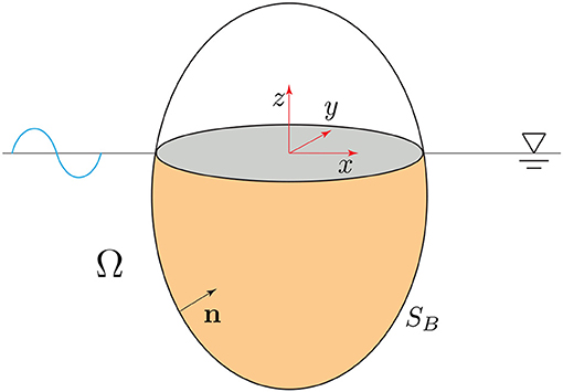
Figure 1. Floating body.

Each potential ϕ_i(x) is governed by an independent Laplace equation,

$\begin{array}{ll}\Delta {\varphi }_i(\text{x})=0& (3)\end{array}$

with $\Delta =(\frac{{\partial }^2}{\partial x^2}+\frac{{\partial }^2}{\partial y^2}+\frac{{\partial }^2}{\partial z^2})$ the Laplace operator.

The free-surface and non-permeable boundary conditions are imposed at z = 0 and z = −h, respectively

$\begin{array}{ll}\frac{\partial {\varphi }_i}{\partial z}-\frac{{\omega }^2}{g}{\varphi }_i=0\mathrm{\text{ in }}z=0& (4)\end{array}$

$\begin{array}{ll}\frac{\partial {\varphi }_i}{\partial z}=0\mathrm{\text{ in }}z=-h& (5)\end{array}$

with g the gravity acceleration constant. At the interphase, both velocities at the solid and fluid are equal. Thus,

$\begin{array}{ll}\frac{\partial {\varphi }_i}{\partial \text{n}}=-\text{i}\omega V_i({\text{a}}_i·\text{n})\mathrm{\text{ in }}{S}_B& (6)\end{array}$

with n the unitary normal vector exterior to the fluid domain, and a_i the velocity vector due to a unitary-amplitude oscillation given at the i degree-of-freedom. Last, the Sommerfeld radiation boundary condition is given as,

$\begin{array}{ll}{\displaystyle \underset{r\to \infty }{lim}}(\frac{\partial {\varphi }_i}{\partial r}-\text{i}k{\varphi }_i)=0& (7)\end{array}$

with $r=\sqrt{x^2+y^2}$, and k the wavenumber, which verifies the following dispersion equation,

$\begin{array}{ll}{\omega }^2=gktanh(kh)& (8)\end{array}$

The mass matrix components (μ_ij) and added damping (λ_ij) are obtained by integration.

$\begin{array}{ll}{\mu }_{ij}=\rho {\displaystyle \underset{S_B}{\int }}\text{Re}\left[{\varphi }_i({\text{a}}_j·\text{n})\right]dS& (9)\end{array}$

$\begin{array}{ll}{\lambda }_{ij}=\rho \omega {\displaystyle \underset{S_B}{\int }}\text{Im}\left[{\varphi }_i({\text{a}}_j·\text{n})\right]dS& (10)\end{array}$

With ρ the fluid density.

2.2. Mild-Slope Equation

The second selected problem is centered in the propagation of gravity waves in a three-dimensional fluid domain characterized by a slow-varying depth profile. The governing equation is known as the Mild-Slope equation, proposed by Berkhoff (1972, 1976), in the context of harbor problems. This problem has been solved by numerical methods by the Finite Element Method (e.g., Ortiz and Pastor, 1990; Ortiz and Sánchez, 2001; Ortiz, 2004) for refraction-diffraction. In the BEM literature the domain formulation is explored for particular cases. Isaacson and Qu (1990) develop a method based on Green functions and BEM techniques for predicting the wave field in a harbor containing partially reflecting boundaries. Liu (2001) solves the numerical prediction of combined difraction and refraction ocean waves by use of a Dual Reciprocity BEM (DRBEM).

With reference to Figure 2, a velocity potential Φ(x, t) is considered. The free surface is characterized by the function ς(x, y, t). Function h(x, y) represents the varying depth. In the frequency domain, the complex potential ϕ(x) (1) is introduced. Thus, function ς(x, y, t) can be written as:

$\begin{array}{ll}\varsigma (x,y,t)=\eta (x,y){\text{e}}^{-\text{i}\omega t}& (11)\end{array}$

The complex-valued function η(x, y) represents the wave height, interpreted as a perturbation of the free surface respect to the rest position.

FIGURE 2

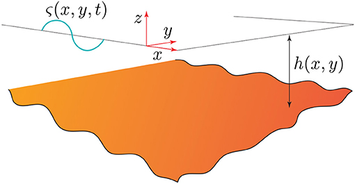
Figure 2. Parameter definition in the Mild-slope problem.

Potential ϕ(x) verifies the Laplace equation, analogous to (3). The impermeable boundary condition at the bottom depth can be written as,

$\begin{array}{ll}\frac{\partial \varphi }{\partial z}+\nabla \varphi ·\nabla h=0\mathrm{\text{ in }}z=-h(x,y)& (12)\end{array}$

with ∇ the gradient operator in the spatial coordinates (x, y). The free-surface condition can be written as,

$\begin{array}{ll}\frac{\partial \varphi }{\partial z}-\frac{{\omega }^2}{g}\varphi =0\mathrm{\text{ in }}z=0& (13)\end{array}$

For the particular case of constant-depth, it can be proved Chamberlain and Porter (1995) that function η(x, y) verifies the Helmholtz equation,

$\begin{array}{ll}\Delta \eta (x,y)+k^2\eta (x,y)=0& (14)\end{array}$

with k the wave length, for which the dispersion Equation (8) is verified.

2.3. Boundary Element Formulation

To approximate the solution by the BEM, the first step is the statement of a Boundary Integral Equation (BIE). For an internal point, (3), and considering the potential ϕ, the BIE is

$\begin{array}{ll}\varphi (\text{x})+{\displaystyle {\int }_S}\frac{\partial G(\text{x};\text{y})}{\partial \text{n}}\varphi (\text{y})\text{d}S(\text{y})={\displaystyle {\int }_S}G(\text{x};\text{y})\frac{\partial \varphi (\text{y})}{\partial \text{n}}\text{d}S(\text{y})& (15)\end{array}$

with x ∈ Ω, y ∈ S, and G(x; y) is the Green function of the problem; for the three-dimensional Laplace equation, the Green function is,

$\begin{array}{ll}G(\text{x};\text{y})=\frac{1}{4\pi r(\text{x};\text{y})}& (16)\end{array}$

with r(x; y) the euclidean distance from point x, or collocation point to the observation point y.

The BIE for a smooth boundary point x ∈ S is obtained after a limit-to-the-boundary process (Brebbia and Dominguez, 1996; Bonnet, 1999)

$\begin{array}{ll}\frac{\varphi (\text{x})}{2}+{\displaystyle {\int }_S}\frac{\partial G(\text{x};\text{y})}{\partial \text{n}}\varphi (\text{y})\text{d}S(\text{y})={\displaystyle {\int }_S}G(\text{x};\text{y})\frac{\partial \varphi (\text{y})}{\partial \text{n}}\text{d}S(\text{y})& (17)\end{array}$

Both BIEs (15, 17) are valid for the Helmholtz Equation (14), considering a bi-dimensional domain and replacing variable ϕ by η, with the Green function,

$\begin{array}{ll}G(x;y)=\frac{1}{2\pi }{K}_0(\text{i}kr)& (18)\end{array}$

with K₀ the modified Bessel function order 0. In Isaacson and Qu (1990) it is derived an alternative expression for this Green function in the context of the Mild-slope equation. In case of variable-depth, the Dual Reciprocity Method (Liu, 2001) leads to a BEM formulation.

Equation (17) is used in a standard collocation method. After the boundary discretization, and integral evaluation, it is obtained the basic matrix formulation, as follows

$\begin{array}{ll}\text{H}\text{U}=\text{G}\text{Q}& (19)\end{array}$

with H and G two matrices, and U and Q vectors with degrees-of-freedom in potential ϕ or flux $\frac{\partial \varphi }{\partial \text{n}}$, respectively. After the application of the prescribed boundary condition, the linear system of equations is obtained,

$\begin{array}{ll}\text{A}\text{X}=\text{B}& (20)\end{array}$

The evaluation of the integrals depends on the type of shape functions selected to interpolate the potential or flux variables (Brebbia and Dominguez, 1996), with particularities for singular or quasi-singular integration. In this paper constant elements have been considered, due to its widely use in the literature about acceleration techniques in BEM.

3. A Parallel GMRES With CUDA

3.1. The Generalized Minimum Residual Method

In this section the restarted GMRES (van der Vorst, 2003) is described. With reference to system (20), the first step in the GMRES solver is the definition of an initial solution vector, X₀. Thus, a first residual is defined as r₀ = B−A·X₀. Algorithm 1 describes the steps of the restarted GMRES, in which a new initial point X₀ is set after m steps, unless the convergence criteria is reached. This technique allows important reductions in memory and computing times. In the context of this paper, the GMRES schema has been adapted to incorporate complex-valued matrices and operations.

ALGORITHM 1

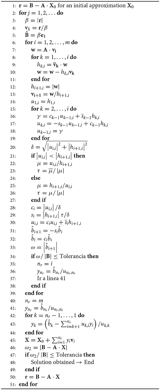
Algorithm 1: Restarted GMRES

With reference to Algorithm 1, vector e₁, length m, is a unitary vector, in which the first position is 1 and 0 the other positions. The dot products with complex-valued components are interpreted in the sense of the inner product in a Hilbert space. Thus, if a and b are complex-valued vector, the dot product is defined as follows,

$\begin{array}{ll}\text{a}·\text{b}=\sum \overline{a_i}·b_i.& (21)\end{array}$

with ${\overline{a}}_i$ the complex-conjugate of term a_i. The sum (21) is extended to the dimension of the complex vector.

The norm |v| is defined in terms of the previously defined product,

$\begin{array}{ll}\left|\text{v}\right|=\sqrt{\sum {\overline{v}}_i{v}_i}& (22)\end{array}$

The stopping criterion is an important aspect in solver iterative algorithms. In the context of this work, a dimensionless norm has been considered, reported in Frayssé et al. (1998).

$\begin{array}{ll}\frac{\left|\text{r}\right|}{\alpha \left|\text{x}\right|+\chi }\le \mathrm{\text{Tolerance}}& (23)\end{array}$

with α and χ two parameters to be set up by the user. In this paper, parameters α = 1 and χ = 0 have been considered.

3.2. GPU Parallelization With CUDA

In the GMRES, the most demanding operation is the calculation of the matrix-vector products. The parallelization of these products has been implemented in CUDA programming languaje and run in the GPU. The GPU is a device with specific resources that must be considered in the design of the algorithms.

Computing times are sensitive to particular aspects, such as the use of the shared memory, registers per thread and the block-threads structure of the computing grid Kirk and Hwu (2012). These parameters determine the occupancy¹ of the GPU. CUDA allows the code to be optimized for each particular GPU device, which cause portability and scalability of the generated codes. To adapt the execution parameters to each singular GPU, the CUDA Occupancy Calculator developed by NVidia has been used. Given the shared memory and the number of registers per thread, the highest value of number of threads per block are optimized for any particular GPU device.

Figure 3 shows the global schema for the proposed solver. The operations are grouped into four steps: two of them are carried out in the CPU, and two into the GPU device.

FIGURE 3

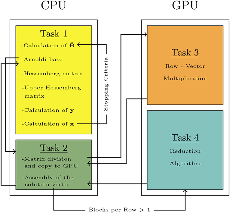
Figure 3. Solver: global schema.

Algorithm 2 is implemented with CUDA to be run in the GPU. This algorithm is focused on control of the matrix-vector products. Given a matrix M and vector V, the grid structure is determined depending on the matrix and vector dimensions, for maximum GPU occupancy. In general, for systems with large number of degrees of freedom it is required the use of more than one block per row, in order to balance the number of operations required to process each row. However, when more than one block is required per row, results computed at each block must to be reduced to a unique value per row.

ALGORITHM 2

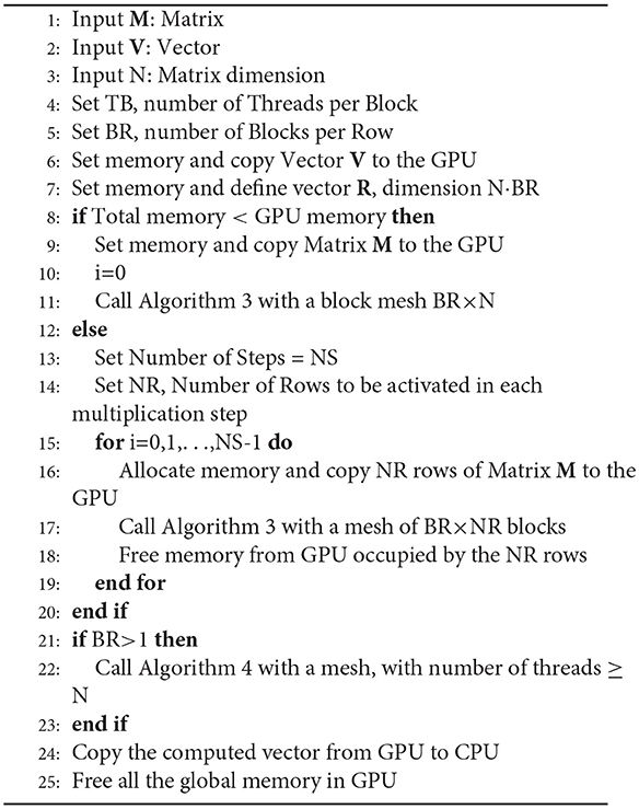
Algorithm 2: Matrix-Vector product - Main (CPU)

After the definition of these setup parameters, the memory transfer operations between GPU and CPU must be minimized. In this sense, the system matrix in the BEM code is fully populated; thus, no compression methods are available, and all the components of the matrix must be transferred to the GPU. This transference is carried out by splitting the matrix in sub-matrices. Each sub-matrix block is transferred to the GPU, in which the matrix-vector product is carried out.

Algorithm 3 describes the first set of operations run in the GPU. Each thread is used to carry out the product of the matrix elements by the vector. Results are stored in a local vector in the shared memory at each block. The reading/writing access to the shared memory are faster than global memory.

ALGORITHM 3

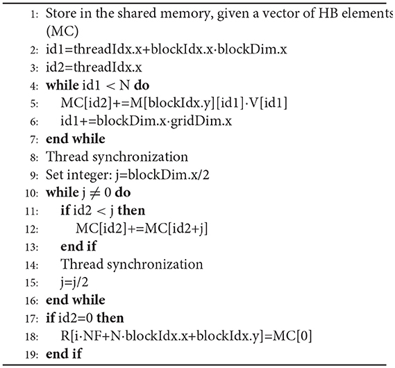
Algorithm 3: Matrix-Vector Product - GPU product

The next step is the addition of the vector elements in each thread in the shared memory, obtaining a unique value per block. This addition is stored in a vector R in the global memory of the GPU.

The second step to be carried out in the GPU is described by Algorithm 4. The aim of this part is the addition of the individual values obtained at each block, in order to give the resulting vector. This part is only required in case of defining more than one block per row of matrix M. The last step is copying the N first elements in vector R to the RAM memory in CPU.

ALGORITHM 4

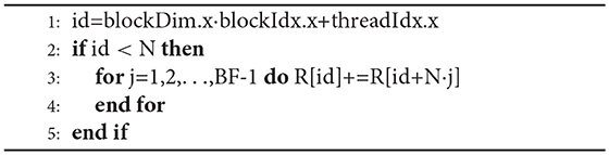
Algorithm 4: Matrix-Vector Product - Reduction in (GPU)

4. Numerical Tests

The proposed GMRES has been implemented in C++ and CUDA, in the context of two BEM codes. The main objective of the tests is the direct comparison of the computing times required by the parallel GPU solver, compared with a pure sequential CPU implementation. Tests are designed to measure the performances of the parallel solver in the GPU. Thus, the CPU operations have not been parallelized. No additional compiler optimizations have been used in CPU, which could cause wrong conclusions about computing times associated with the tested algorithms.

The NVidia GeForce GTX 1080 graphic card has been used, with a compute capability 6.1, 8GB in global memory, 48KB of shared memory per block, and 20 multiprocessors type SPMD (Single Program Multiple Data), with 128 CUDA cores per multiprocessor. CUDA 10 version has been used. The GPU allows a maximum of 1024 threads per block and 2048 threads per multiprocessor. For Algorithm 3, the code allocates 22 registers per thread and the required shared memory is 16 bytes (size of a double precision complex number) per thread. On the other hand, for Algorithm 4, the code computes 28 registers per thread and no shared memory is required. With these values, the occupancy calculator selects 1,024 threads per block with 100% occupancy. The CPU is an Intel i7-6800K processor.

The Salome mesher (http://www.salome-platform.org/) has been used to generate the three-dimensional meshes in the floating body problem. The post-processing software Paraview (http://www.paraview.org/) has been used to visualize the results.

4.1. Added Mass of a Floating Cylinder

This first example is in the context of fluid-solid interaction analysis. In this problem, term μ₁₁ in (9), corresponding to a time-harmonic movement in direction x, is solved. The floating body is a cylinder, shown in Figure 4, as a function of the wavelength. This problem has an analytic solution in terms of a normal modes expansion (Bhatta, 2003). The objective is the observation of the dependence on the frequency on the computing times at a fixed mesh.

FIGURE 4

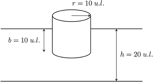
Figure 4. Floating cylinder.

The number of elements of the computing mesh is 7568, shown in Figures 5 and 6. Constant three-node elements are used. The minimum element size has been selected according to a criterium dependent on the minimum wavelength, associated with the higher frequency. Ten elements per minumum wavelength have been considered.

FIGURE 5

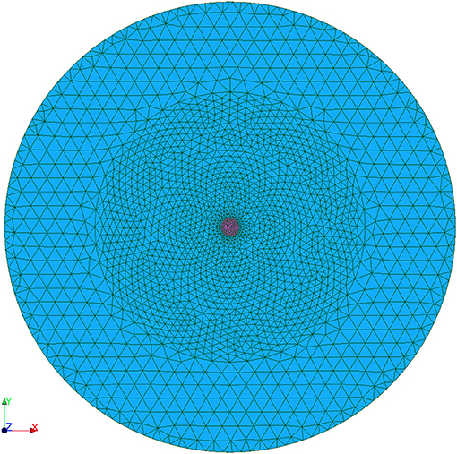
Figure 5. Floating body problem. 3D Mesh, seen from above.

FIGURE 6

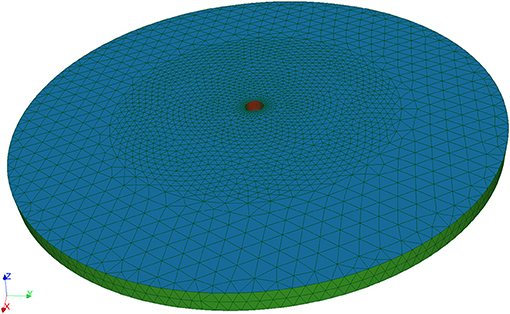
Figure 6. Floating body problem. 3D Mesh, perspective.

The Laplace Equation (3), with the boundary conditions given by Equations (4–6) have been considered. The radiation condition (7) has been set in a simplified way Ortiz and Pastor (1990), because the Green function considered does not fulfill the radiation boundary condition. An external boundary has been defined in r = 250 u.l. (units of length), for which relation (7) is established. In this way, a complex-valued boundary condition is given, which allows progressive waves in the solution. This approximation avoids matching with an external solution based on a normal-mode expansion, with a good approximation in the frequency range tested.

Figure 7 shows the results for the added mass. Values computed by integration (9) are compared, when potential function is obtained by the BEM or by the analytic solution reported in Bhatta (2003). The dimensionless variable kr is shown in abscissas, in which r is the cylinder radius and k the wavenumber. The Y-axis represents the dimensionless values of the added mass μ₁₁. Small differences between the added mass values are observed, less than 2%. Note that the comparison is in integrated values of the computed potential, and not in the potential itself. Both solutions includes representation errors; the analytic solution is given in series form, in which the singular behavior in corner is not included (Guzina et al., 2006). In contrast, the BEM solution is obtained with constant elements, and the radiation boundary condition is imposed in an approximate form.

FIGURE 7

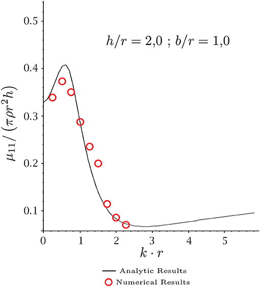
Figure 7. Added mass μ₁₁, as a function of k·r.

Table 1 shows the computing times required, as a function of the wavelength. Column CPU shows the times required by the GMRES in CPU (sequential). Column GPU shows the computing times required by the GMRES in GPU. The last column shows the speedup, computed as the rate between the CPU and GPU times. It is observed a dependence in the computing times with respect to the wavelength. The parallel GMRES is more effective at low frequencies. This is due to the fixed mesh considered in all the tests, with constant elements. The solution with constant elements is poor for high frequency. The GMRES algorithm shows poor convergence, and more iterations are required. At low frequency, fast convergence is observed.

TABLE 1

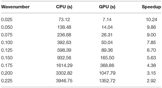
Table 1. Computing times in the floating cylinder problem.

4.2. Internal Harbor Oscillations

In this section, the Mild-Slope equation is solved by the BEM, to characterize the internal waves in a harbor. This problem has been studied by Isaacson and Qu (1990); the same conditions have been adopted in this paper.

Figure 8 shows the harbor geometry. The incidental wave η^I is characterized by a period 2.0 u.t (units of time), amplitude 0.5 u.l. (units of legth) and a propagation direction perpendicular to the harbor opening. Absorbing boundaries are considered at the harbor. Constant depth, 20 u.l. is considered.

FIGURE 8

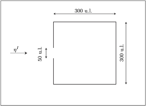
Figure 8. Harbor configuration.

The Helmholtz Equation (14) is solved, for the wave elevation η. The numerical results obtained for η inside the harbor domain are shown in Figure 9. Note that this case corresponds with a high frequency problem, with short wavelengths.

FIGURE 9

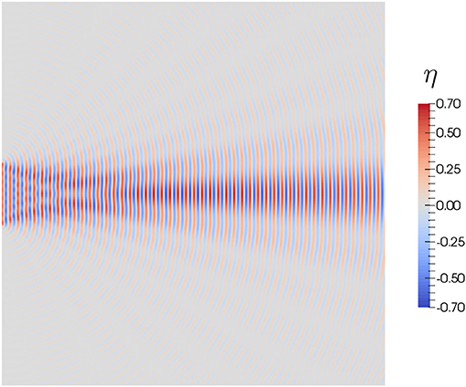
Figure 9. Internal solution for η.

In this problem different meshes have been used, in order to observe the efficiency of the GPU parallelization when the number of degrees of freedom is increased. Table 2 shows the computing times; column DOF reports the number of degrees of freedom in the system; column Collocation shows the computing time required by the BEM to generate the system matrix and vector; columns CPU y GPU show the computing times required by the GMRES solved in CPU or GPU, respectively. The last column shows the speedup of the GPU solver.

TABLE 2

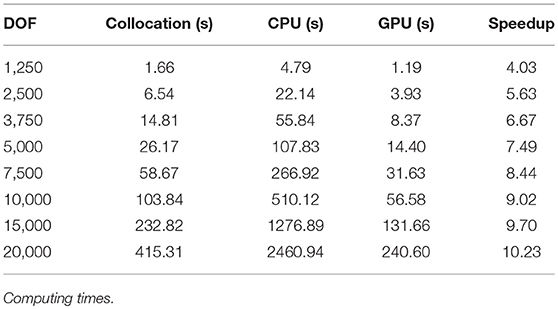
Table 2. Harbor oscillations.

Numerical results shows that computing times required by the collocation BEM (both in CPU) are one order less to the computing times required to solve the linear system of equations. It is also shown that the GPU solver is more efficient for large number of degrees of freedom. For small number of degrees of freedom, the bottleneck comes from time required to transfer memory from CPU to the global memory in GPU. The speedup increases for large number of degrees of freedom, even in systems with 15,000 and 20,000 equations, in which the product matrix-vector is carried out by blocks, with multiple memory transferences from GPU to CPU.

5. Concluding Remarks

In this paper, a GPU implementation of the GMRES algorithm is presented in the context of the BEM with fully-populated matrices and with complex-valued arguments. It is explored an interesting field related to the acceleration techniques for the BEM in the frequency domain. With difference to other acceleration techniques for the BEM (FMM, pFFT or ACA), the proposed approach does not require modifications in the main program, which computes the system matrix and the right vector. This allows the use of standard BEM codes, with the solver task transferred to the GPU.

The GMRES version described here does not include a pre-conditioner. The use of preconditioners in the GMRES and BEM is an important aspect for particular problems with poorly conditioned matrices. In the context of this paper, numerical tests have been designed to show the performances of the proposed solver. The development of a general preconditioned GMRES in GPU for the BEM is out of the scope of this paper.

The acceleration is carried out by a main task controlled in the CPU, which allows the massive parallelization of the matrix-vector products in the GPU. The CUDA programming language has been used to implement an adaptive solver, in the sense that the generated code is optimized for the particular GPU device in which it is compiled. The generated solver is portable and scalable for future GPU devices. All the different GPU and CPU tasks are described in algorithmic language.

Numerical tests show time reductions when compared with a standard CPU solver. In the context of the BEM, the inherent reduction in the number of degrees of freedom (only at the boundary) causes that the standard collocation method, with a direct assembly of the system matrix and right vector, is extended among the different numerical codes for a wide number of applications. For such codes, the proposed solver represents an easy way to obtain time reductions in computing times by transferring the solver task to the GPU. Due to the fast development of the GPU systems, with improvements in the number of cores, increasing the device memories and improving the speed of the memory transferences, the proposed GPU solver shows an interesting way of acceleration, with future improvements depending on the device developments.

Author Contributions

AM-C conceived of the presented idea. JM-M, AM-C, and PO developed the theoretical formalism and designed the numerical tests. JM-M developed the presented algorithms and implemented them on a computational framework. He also performed the calculations and generated tables and figures. JM-M, AM-C, and PO contributed to the final version of the manuscript.

Conflict of Interest Statement

The authors declare that the research was conducted in the absence of any commercial or financial relationships that could be construed as a potential conflict of interest.

Acknowledgments

We appreciate the partial financial support from the MINECO/FEDER project BIA2015-64994-P.

Footnotes

1. ^Number of simultaneous threads computed by multiprocessor divided by the maximum allowed.

References

Benedetti, I., Aliabadi, M., and Daví, G. (2008). A fast 3D dual boundary element method based on hierarchical matrices. Int. J. Solids. Struct. 45, 2355–2376. doi: 10.1016/j.ijsolstr.2007.11.018

CrossRef Full Text | Google Scholar

Berkhoff, J. C. W. (1972). “Computation of combined refraction-diffraction,” in Proceedings of the 13th International Conference on Coastal Engineering (Vancouver, BC), 471–490.

Google Scholar

Berkhoff, J. C. W. (1976). Mathematical Models for Simple Harmonic Linear Water Wave Models; Wave Refraction and Diffraction. Ph.D. thesis, Delf University of Technology.

Bhatta, D. D. (2003). Surge Motion on a floating cylinder in water of finite depth. Int. J. Math. Math. Sci. 2003, 3643–3656. doi: 10.1155/S0161171203209285

CrossRef Full Text | Google Scholar

Bonnet, M. (1999). Boundary Integral Equation Methods for Solids and Fluids. Chichester: Wiley.

Google Scholar

Brancati, A., and Aliabadi, M. H. I. B. (2009). Hierarchical adaptive cross approximation GMRES technique for solution of acoustic problems using the boundary element method. Comput. Model. Eng. Sci. 43, 149–172. doi: 10.3970/cmes.2009.043.149

CrossRef Full Text | Google Scholar

Brebbia, C. (1978). The Boundary Element Method for Engineers. New York, NY: Pentech Press; Halstead Press.

Google Scholar

Brebbia, C., and Dominguez, J. (1996). Boundary Elements: An Introductory Course. Southampton: WIT Press.

Google Scholar

Brebbia, C. A., and Partridge, P. W. (1992). Boundary Elements in Fluid Dynamics. Southampton: Springer.

Google Scholar

Chaillat, S., and Bonnet, M. (2013). Recent advances on the fast multipole accelerated boundary element method for 3D time-harmonic elastodynamics. Wave Motion 50, 1090–1104. doi: 10.1016/j.wavemoti.2013.03.008

CrossRef Full Text | Google Scholar

Chamberlain, P. G., and Porter, D. (1995). The modified mild-slope equation. J. Fluid Mech. 291, 393–407. doi: 10.1017/S0022112095002758

CrossRef Full Text | Google Scholar

Cheng, A. D. H., and Cheng, D. T. (2005). Heritage and early history of the boundary element method. Eng. Anal. Boundary Elem. 29, 268–302. doi: 10.1016/j.enganabound.2004.12.001

CrossRef Full Text | Google Scholar

D'Azevedo, E., and Nintcheu Fata, S. (2012). On the effective implementation of a boundary element code on graphics processing units using an out-of-core LU algorithm. Eng. Anal. Boundary Elem. 36, 1246–1255. doi: 10.1016/j.enganabound.2012.02.014

CrossRef Full Text | Google Scholar

Djojodihardjo, H. (2010). “Further development in the application of fast multipole boundary element method for unified BEM-FEM acoustic-structural coupling,” in 61st International Astronautical Congress 2010, IAC 2010, vol. 4, Prague, 3417–3429.

Google Scholar

Frayssé, V., Giraud, L., and Gratton, S. (1998). A Set of Flexible-GMRES Routines for Real and Complex Arithmetics. Technical report, Centre Européen de Recherche et de Formation Avancée en Calcul Scientifique TR/PA/98/20.

Google Scholar

Geng, W., and Jacob, F. (2013). A GPU-accelerated direct-sum boundary integral Poisson–Boltzmann solver. Comput. Phys. Commun. 184, 1490–1496. doi: 10.1016/j.cpc.2013.01.017

CrossRef Full Text | Google Scholar

Gumerov, N. A., and Duraiswami, R. (2005). Fast Multipole Methods for the Helmholtz Equation in Three Dimensions. Amsterdam: Elsevier.

Google Scholar

Guzina, B. B., Pak, R. Y. S., and Martínez-Castro, A. (2006). Singular boundary elements for three-dimensional elasticity problems. Eng. Anal. Bound. Elem. 30, 623–639. doi: 10.1016/j.enganabound.2006.02.010

CrossRef Full Text | Google Scholar

Hackbusch, W. (1999). A sparse matrix arithmetic based on hierarchical matrices. Part I: introduction to hierarchical matrices. Computing 62, 89–108. doi: 10.1007/s006070050015

CrossRef Full Text | Google Scholar

Hamada, T., and Takahashi, T. (2009). GPU-accelerated boundary element method for Helmholtz equation in three dimensions. Int. J. Numer. Meth. Eng. 80, 1295–1321. doi: 10.1002/nme.2661

CrossRef Full Text | Google Scholar

Hess, J. L. (1990). Panel methods in computational fluid dynamics. Annu. Rev. Fluid Mech. 22, 255–274. doi: 10.1146/annurev.fl.22.010190.001351

CrossRef Full Text | Google Scholar

Isaacson, M., and Qu, S. (1990). Waves in a harbour with partially reflecting boundaries. Coast. Eng. 14:193–214. doi: 10.1016/0378-3839(90)90024-Q

CrossRef Full Text | Google Scholar

Jaswon, M. A., and Porter, A. R. (1963). An integral equation solution of the torsion problem. Proc. R. Soc. 273, 237–246. doi: 10.1098/rspa.1963.0085

CrossRef Full Text | Google Scholar

Kelly, J. M., Divo, E. A., and Kassab, A. J. (2014). Numerical solution of the two-phase incompressible Navier–Stokes equations using a GPU-accelerated meshless method. Eng. Anal. Boundary Elem. 40, 36–49. doi: 10.1016/j.enganabound.2013.11.015

CrossRef Full Text | Google Scholar

Kirk, D., and Hwu, W. (2012). Programming Massively Parallel Processors: A Hands-on Approach. Cambridge, MA: Morgan Kaufmann.

Google Scholar

Leung, C., and Walker, S. P. (1997). Iterative solution of large three-dimensional BEM elastostatic analyses using the GMRES technique. Int. J. Numer. Meth. Eng. 40, 2227–2236.

Google Scholar

Li, R., and Saad, Y. (2013). GPU-accelerated preconditioned iterative linear solvers. J. Supercomput. 63, 443–466. doi: 10.1007/s11227-012-0825-3

CrossRef Full Text | Google Scholar

Liu, H.-W. (2001). Numerical Modelling of the Propagation of Ocean Waves. Ph.D. thesis, University of Wollongong.

Liu, Y. (2009). Fast Multipole Boundary Element Method. New York, NY: Cambridge University Press.

Google Scholar

Liu, Y., and Nishimura, N. (2006). The fast multipole boundary element method for potential problems: a tutorial. Eng. Anal. Bound. Elem. 30, 371–381. doi: 10.1016/j.enganabound.2005.11.006

CrossRef Full Text | Google Scholar

Liu, Y. J. (2008). A fast multipole boundary element method for 2D multi-domain elastostatic problems based on a dual BIE formulation. Comput. Mech. 42, 761–773. doi: 10.1007/s00466-008-0274-2

CrossRef Full Text | Google Scholar

Liu, Y. J., Mukherjee, S., Nishimura, N., Schanz, M., Ye, W., Sutradhar, A., et al. (2012). Recent advances and emerging applications of the boundary element method. Appl. Mech. Rev. 64, 1–38. doi: 10.1115/1.4005491

CrossRef Full Text | Google Scholar

López-Portugués, M., López-Fernández, J., Menéndez-Canal, J., Rodríguez-Campa, A., and Ranilla, J. (2012). Acoustic scattering solver based on single level FMM for multi-GPU systems. J. Parallel Distr. Com. 72, 1057–1064. doi: 10.1016/j.jpdc.2011.07.013

CrossRef Full Text | Google Scholar

Lu, T., Wang, Z., and Yu, W. (2004). Hierarchical block boundary-element method (HBBEM): a fast field solver for 3-D capacitance extraction. IEEE T. Microw. Theory 52, 10–19. doi: 10.1109/TMTT.2003.821228

CrossRef Full Text | Google Scholar

Ma, Z., Wang, H., and Pu, S. (2014). GPU computing of compressible flow problems by a meshless method with space-filling curves. J. Comput. Phys. 263, 113–135. doi: 10.1016/j.jcp.2014.01.023

CrossRef Full Text | Google Scholar

Margonari, M., and Bonnet, M. (2005). Fast multipole method applied to the coupling of elastostatic BEM with FEM. Comput. Struct. 83, 700–717. doi: 10.1016/j.compstruc.2004.09.007

CrossRef Full Text | Google Scholar

Mei, C. C., Stiassnie, M., and Yue, D. K. P. (2005). Theory and Applications of Ocean Surface Waves. London: World Scientific Publishing Company.

Google Scholar

Ortiz, P. (2004). Finite Elements using a plane-wave basis for scattering of surface water waves. Philos. Trans. R. Soc. A. 362, 525–540. doi: 10.1098/rsta.2003.1333

PubMed Abstract | CrossRef Full Text | Google Scholar

Ortiz, P., and Pastor, M. (1990). Un modelo numérico de refracción-difracción de ondas en zonas costeras. Rev. Int. Metod. Numer. 6, 409–436.

Google Scholar

Ortiz, P., and Sánchez, E. (2001). An improved partition of unity finite element model for diffraction problems. Int. J. Numer. Meth. Eng. 50, 2727–2740. doi: 10.1002/nme.161

CrossRef Full Text | Google Scholar

Phillips, J. R. (1997). Rapid Solution of Potential Integral Equations in Complicated 3–Dimensional Geometries. Ph.D. thesis, MIT.

Phillips, J. R., and White, J. K. (1997). A Pre-Corrected-FFT Method for Electrostatic Analysis of Complicated 3–D Structures. IEEE Trans. Comput. Aided Des. 16, 1059–1072. doi: 10.1109/43.662670

CrossRef Full Text | Google Scholar

Rokhlin, V. (1985). Rapid solution of integral equations of classical potential theory. J. Comput. Phys. 60, 187–207. doi: 10.1016/0021-9991(85)90002-6

CrossRef Full Text | Google Scholar

Saad, Y., and Shultz, M. (1986). GMRES: a generaliced minimal residual algorithm for solving non-symmetric linear systems. SIAM J. Sci. Stat. Comput. 7, 856–869. doi: 10.1137/0907058

CrossRef Full Text | Google Scholar

Sanders, J., and Kandrot, E. (2010). CUDA by Example. Boston, MA: Addison-Wesley.

Google Scholar

van der Vorst, H. (2003). Iterative Krylov Methods for Large Linear System. Cambridge, UK: Cambridge University Press.

Google Scholar

Wang, G., Wang, Q. F., and Wang, Y. J. (2011). GPU based boundary element analysis for 3D elastostatics with GMRES-DC algorithm solving system equations. Adv. Mat. Res., 308–310, 2345–2348. doi: 10.4028/www.scientific.net/AMR.308-310.2345

CrossRef Full Text | Google Scholar

Wang, Y., Wang, Q., Wang, G., Huang, Y., and Wang, S. (2013). An adaptive dual-information FMBEM for 3D elasticity and its GPU implementation. Eng. Anal. Boundary Elem. 37, 236–249. doi: 10.1016/j.enganabound.2012.09.012

CrossRef Full Text | Google Scholar