An Application of Semi-empirical Physical Model of Tsunami-Bore Pressure on Buildings

Introduction

The 2011 Tohoku earthquake tsunami struck a wide area of the northeastern coast of Japan and caused extensive infrastructure damage. In the last decade, tsunami wave pressure has been investigated by many researchers, and its characteristics are becoming clear (e.g., Arikawa et al., 2005; Nouri et al., 2010).

Fukui et al. (1963) and Arikawa et al. (2005, 2006) reported that two characteristic patterns were observed in pressures on structures. In the experiment of Fukui et al. (1963), pressures exerted by bores, which were generated by rapidly opening a hinged gate, on a levee with a sloped face on the seaside were measured. In the experiment of Arikawa et al. (2005, 2006), pressures on a rectangular block were measured under the condition of long sinusoidal waves with periods in the range of 14–60 s. The first pressure pattern observed by both experiments was called the impulsive-bore pressure and was observed just after the bore impacted the structures. The vertical profile of the impulsive-bore pressure is a non-hydrostatic form. The second one was called the continuous pressure, or quasi-steady-state pressure, and was observed after the reflection of bores. The vertical profile of the continuous pressure or quasi-steady-state pressure is a hydrostatic form.

Nouri et al. (2010), Palermo et al. (2013), and Kihara et al. (2015) divided the impulsive-bore pressure into two phases. The first one is the impulsive pressure and is observed just after the tsunami impacted the buildings, and its duration is very short, generally shorter than 1 s. The second one is the run-up or initial-reflection-phase pressure and is observed during the transition between the impulsive and quasi-steady hydrodynamic forces. In this study, the “impulsive-bore pressure” is divided into the “impulsive pressure” and the “bore pressure.”

Some researchers have studied bore pressure characteristics and profiles (e.g., Matsutomi, 1991). In the experiment of Cross (1967), a column of water was deflected upward when a bore front struck the wall, and peak forces were observed when the column of water collapsed onto the bore. In the experiments conducted by Ramsden and Raichlen (1990) and Ramsden (1996), the maximum force was measured after the maximum run-up was reached, as was the case in the experiments conducted by Cross (1967). Palermo et al. (2013) also reported that the horizontal forces on the structures measured when the bore ran up the wall were greater than the impulsive force in their experiment. These results indicate that the wave forces due to the bore pressures sometimes become higher than those due to the impulsive pressures. Matsutomi (1991) experimentally investigated characteristics of bore pressure on a vertical wall. In the experiments, the bore was generated by rapidly opening a gate. Matsutomi (1991) showed the relationship between bore profiles and the pressure distributions, and that the vertical distribution of the bore pressure was parabolic.

Characteristics of tsunami wave pressures have also been investigated by numerical simulations (e.g., St-Germain et al., 2013; Douglas and Nistor, 2015; Sarjamee et al., 2017a,b). Douglas and Nistor (2015) and Sarjamee et al. (2017a) investigated tsunami wave force by carrying out three-dimensional hydrodynamic numerical simulations with the open source computational fluid dynamics library OpenFOAM with the interFoam solver, which is a two-phase and incompressible fluid solver. In this solver, the air-water boundary is solved by volume of fluid method. In these studies, predicted tsunami wave forces on a square column with initially both the dry and wet bed conditions were compared with those measured by physical experiments of Al-Faesly et al. (2012). These study shows that predicted forces due to bore pressure are in good agreement with the measured ones. St-Germain et al. (2013) and Wei et al. (2015) investigated tsunami wave force by carrying out three-dimensional numerical simulations with Smoothed-Particle Hydrodynamics methods. These studies also show that predicted forces due to bore pressure are in good agreement with measured ones.

These numerical studies show that by carrying out three-dimensional hydrodynamic simulations, hydrodynamic forces due to bore pressure on structures are able to be reproduced. However, good-reproduction of the characteristics and profiles of the tsunami wave pressures need high resolutions in horizontal and vertical directions since good-reproductions of details of flow patterns in front of the structures are needed for good reproduction of the profiles of impulsive and bore pressures. Thus, numerical costs becomes very expensive for solving wide inundation areas of actual tsunamis by three-dimensional numerical simulations.

Kihara and Kaida (2016) carried out hydraulic experiments for investigation of characteristics of the bore pressure. In the experiment, bores were generated by rapidly opening a gate and they impacted a vertical wall on a dry bed. They showed that positive pressures were measured much lower than the top level of the water column on the vertical wall, and the pressures were negligibly low at the top level of the water column. In the study, a physical model of bore pressures was proposed by applying the turbulent bore theory of Madsen and Svendsen (1983). Bore pressures can be evaluated by coupling the physical model with horizontally two-dimensional simulations of nonlinear shallow water equation models, by which hydrodynamic pressures are not able to be solved but inundation depths and velocities in wide inundation areas can be solved with much lower numerical costs than those of three-dimensional numerical simulations.

On the other hand, there are some issues in the physical model proposed by Kihara and Kaida (2016) on practical uses. The first issue is that the model is too complicated. In the physical model, by using time series of inflow conditions, time evolutions of length of reflected waves and flow properties in the reflected waves at the position of the wall under conditions where there are no walls are calculated. For the calculation, seven equations are iteratively solved for each time step, and the iterative calculation did not sometimes convergence. The second issue is that it is difficult to obtain input parameters of the physical model, since time series of inflow conditions, which have no effect on the buildings, are needed for the evaluation of bore pressures on buildings by solving the physical model.

In this study, by using the experimental data of Kihara and Kaida (2016), characteristics of bore pressure are shown, and a semi-empirical physical model of bore pressure is developed, by which bore pressures are evaluated from the numerical results of inundation simulations by two-dimensional nonlinear shallow water equation models. This paper is organized as follows. First, Experiments describes the experiment of Kihara and Kaida (2016), and Experimental results describes the flow and pressure profiles observed in the experiment. In Semi-empirical physical model of bore pressure, we develop a semi-empirical physical model of bore pressure, which is based on that proposed by Kihara and Kaida (2016), but is modified for practical applications. In Practical application method of semi-empirical physical model of bore pressure, we propose an application method of the semi-empirical physical model of bore pressure. In Application of semi-empirical physical model to an inundation simulation, we apply the semi-empirical physical model to evaluations of pressure acting on buildings in an inundation area by carrying out numerical simulation of tsunami inundation.

Experiments

Kihara and Kaida (2016) carried out a series of experiments using CRIEPI's Large-scale Tsunami Physical Simulator (Kihara, 2016). The test section is an open channel made of reinforced concrete that is 20 m long, 4 m wide, and 2.5 m high. On the upstream side of the test section, a closed rectangular channel that is 14.4 m long, 4 m wide, and 2.5 m high is set. A radial steel gate separates the test section and the closed rectangular channel.

The vertical wall was set on the flat bottom in the test flume. The vertical wall was a concrete structure 1.5 m in height, 1.0 m in width, and 0.15 m in thickness. We measured the pressures on the upstream face of the vertical wall. The location of the vertical wall and the velocity and water depth measurement points are shown in Figure 1, along with the coordinate system. The x, y, and z axes denote the streamwise, transverse, and vertical directions, respectively. The origin of the coordinate system is set at the intersection of the center of the vertical wall in the x and y coordinate and the flume bottom. The term u (u, v, w) denotes the velocity vector of x in the (x, y, z) coordinate system.

FIGURE 1

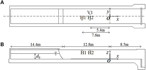
Figure 1. Plane and elevation views of set up of experiment. Definition of coordinate, and location of the vertical wall and measurement points of velocity and water depth are depicted. (A) plane view, (B) elevation view.

Before each experiment, the water depth in the closed rectangular channel was set at a specific water depth d₀. The radial gate was rapidly opened just after each experiment started, and a bore was generated that traveled toward the positive x direction. In each set of experiments, five types of bores were generated by changing the water depth d₀. The water depth d₀ for each bore type is shown in Table 1. It should be noted that the bore generated in this experiment was not the theoretical dambreak flow (e.g., Stansby et al., 1998; Stoker, 2011), which is generated by an instantaneously released or dissolved gate since the release speed of the radial gate is approximately 1 m/s in this experiment.

TABLE 1

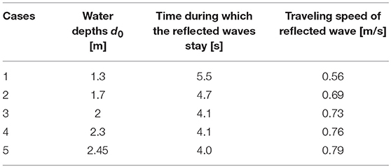
Table 1. The water depth d₀ in the closed rectangular channel, time during which the reflected waves stay, and traveling speed of reflected wave for each case.

The pressures were measured at 23 points along a center line on the upstream face of the vertical wall. Pressure transducers (SSK Co., Ltd., P310) with diameters of 0.01 m, an upper pressure limit of 49 kPa (0.5 kgf /cm²), and a natural frequency of 6.8 kHz were aligned in the vertical direction with the heights of z = 0.01, 0.05, 0.1, 0.15, 0.2, 0.25, 0.3, 0.31, 0.35, 0.4, 0.45, 0.5, 0.55, 0.6, 0.7, 0.8, 0.9, 1.0, 1.1, 1.2, 1.3, 1.4, and 1.49 m.

When a rapid change occurs in temperature, thermal shock is generated in the pressure transducer and erroneous pressure is measured. In the experiment, while the transducers were dry when the experiments started, the transducers became wet after the bore attacked the vertical wall. Since there was temperature difference between the air and the water, the thermal shock tended to take place in our experiment. Thus, Kihara and Kaida (2016) managed to minimize the effects of the thermal shock by carrying out the same measures of Kihara et al. (2015). In order to minimize the effects of the thermal shock, the water was kept placing on the wall until just before each experiment started. Furthermore, when each test finished, the water was impounded in the test flume, and we checked whether measured pressure profiles were equal to the hydrostatic profiles of the water depth. Most of the cases, it was confirmed that the errors were < 0.05 m of the pressure head. The cases in which the measured pressure had errors >0.05 m of the pressure head were excluded in the discussion of the present study.

The water levels/depths were measured at three points, H1, H2, and H3, as shown in Figure 1, by using ultrasonic level sensors (Omron Co., Ltd., E4PA-LS400) installed 3.0 m above the flume bottom. Since the velocities measured in this experiment were over 5 m/s, the fixed arm of the electromagnetic velocimeter must be as thick to maintain the stability of its position. And, the diameter of the fixed arm was 0.048 mm. As a result, the fixed arm disturbed flows significantly, and the disturbance affected the pressure measurements. Thus, we conducted separate experiments for the velocity measurements and those for the pressure measurements. In the pressure measurement experiments, velocities were not measured. On the other hand, in the velocity measurement experiments, the vertical wall was not installed in the test section under the same flow conditions as the pressure measurement experiments. The velocities were measured at the height of 0.1 m from the bed of the point V1 (x = −5.4 m) with a two-component (x, z) electromagnetic velocimeter. Measured pressures, water depths, and velocities were recorded in a data logger (Kyowa Electronic Instruments Co., Ltd, EDX-3000A) at a sampling rate of 10 kHz. The time when the water depth measured at H1 began to respond was defined to be t = 0 s.

Experimental Results

Characteristics of Flow Profile

Figure 2 shows the time series distribution of the water depth d and x-direction velocity u measured at the measurement points H2 and V1 in the velocity measurement experiment, and the Froude numbers Fr (= u / (gd)^0.5), where g is the gravitational acceleration. Due to arrival of the bore (t < 1 s), the water depth rapidly rises to approximately 0.2 m. The higher the water storage depth, the higher the maximum value of water depth, and the shorter the time from bore arrival to maximum water depth. With regard to velocity, the higher the water storage depth, and the higher the maximum velocity, and the maximum velocity is observed immediately after bore arrival (1 s < t < 2 s). Except for immediately after bore arrival (t < 2 s) the Froude numbers are distributed almost the same way in all cases, and when t > 2 s, they decrease monotonically in the range 1 < Fr < 3.

FIGURE 2

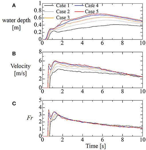
Figure 2. Time series distribution of the water depth d at H2 (A), x-direction velocity u at V1 (B), and the Froude numbers (C).

Figure 3 shows snapshots of the flow in Case 3. Immediately after the bore impacts the vertical wall, a water mass or a water column is observed, which shoots up higher than the top (z = 1.5 m) of the vertical wall (Figure 3B). After the water mass falls, a reflected wave is generated from the vertical wall to the upstream side (Figure 3C), and at the immediate front of the vertical wall, a local rise is observed in the water surface, which reaches the top height of the vertical wall (arrows in Figures 3C,D). As the front of the reflected wave moves away from the vertical wall, the local rise in the water surface on the immediate front of the vertical wall becomes lower (Figures 3E,F).

FIGURE 3

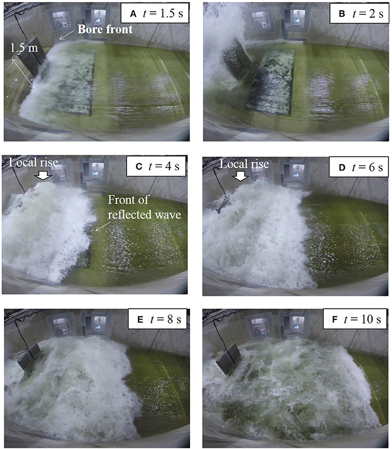
Figure 3. Snapshots of the flow in Case 3. (A) t = 1.5, (B) t = 2, (C) t = 4, (D) t = 6, (E) t = 8, and (F) t = 10 s.

Characteristics of Pressure Profile

The vertical distributions of wave pressure corresponding with the times of the snapshots shown in Figure 3 are shown in Figure 4. Figure 4 shows the pressure head, which is the pressure divided by the product of the water density ρ_w and the gravitational acceleration g. Immediately after a bore impacts the vertical wall, an impulsive pressure is observed, which is greater than the hydrostatic pressure (Figure 4A). After that, although a water column shoots up higher than the top of the vertical wall, a positive wave pressure acts at z < 0.7 m, which is significantly lower than the height of the water column (Figure 4B). Although a local rise is observed in the water surface, which reaches the top height of the vertical wall in Figures 3C,D, positive pressure acts at z < 1 m, which is lower than the height of the local rise (z = 1.5 m) of the water surface (Figures 4C,D). The distribution form of the wave pressure at this time is similar to that when the water column is shooting up and parabolic, as shown in Matsutomi (1991). As the front of the reflected wave moves away from the vertical wall, the pressure distribution approaches the hydrostatic form (Figures 4E, F). In the next section, by considering the above-mentioned relationships between the flow profiles and the bore pressure, which correspond to Figures 4C,D, a semi-empirical physical model of bore pressure is developed.

FIGURE 4

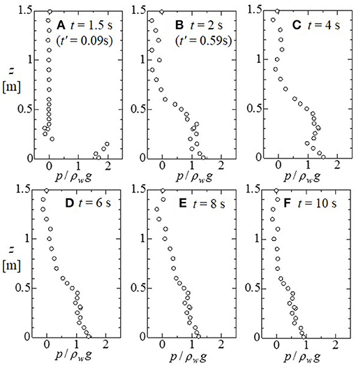
Figure 4. The vertical distributions of wave pressure corresponding with the times of the snapshots shown in Figure 3. (A) t = 1.5, (B) t = 2, (C) t = 4, (D) t = 6, (E) t = 8, and (F) t = 10 s. t' described in (A) and (B) denotes the time elapsed since the bore impacted the vertical wall.

Semi-Empirical Physical Model of Bore Pressure

In this section, a semi-empirical physical model of bore pressures, which is a modified form of Kihara and Kaida (2016), for practical application is developed. In this study, the bore pressure is defined as the pressure observed from the time when the water mass has shot up and fallen to the time when the pressure distribution becomes the hydrostatic form. The time t₀ needed from impact of the bore with the structure until the water mass falls would be related to the propagation speed of the bore U, and could be expressed as

$\begin{array}{cc}\begin{array}{r}{t}_0=c_{0}U/g.\end{array}& (1)\end{array}$

It was confirmed from videos of the experiment that, for all cases, the time needed from impact of the bore with the structure until the water mass falls is given approximately by 3 U/g. It was confirmed from videos of the experiment that, for all cases, the time needed from impact of the bore with the structure until the water mass falls is given approximately by 3 U/g.

In the pressure distribution shown in Figures 4C,D), the heights where non-negligible and positive pressure acts are, respectively, z < 0.8 and z < 1.0 m. Since the inundation depths d of the incident flow measured at measurement point H2 at the same time were 0.53 and 0.62 m, respectively, and the non-negligible wave pressure acts at heights higher than the inundation depth of the incident flow. On the other hand, as described in the previous section, the height of the water surface where a local rise in water level is observed at the immediate front side of the vertical wall, is almost the same height as the top of the vertical wall (z = 1.5 m), and thus the height where the non-negligible wave pressure acts is lower than the height of the local rise of the water surface.

Kihara and Kaida (2016) interpreted the relationship between the bore pressure and the flow property as follows and it is explained together with the conceptual diagram shown in Figure 5A. The reflected wave in a turbulent air/water mixing state (Figure 5A, ii-1, ii-2) occur at the front of the vertical wall. The inflow of the supercritical flow (Figure 5A, i) flows into the front of reflected wave, and a hydraulic jump is observed. The inside of the reflected wave is divided into a high-velocity region at low height (Figure 5A, ii-1) and a turbulent region at high height (Figure 5A, ii-2). As the distance from the front of the reflected wave increases, the high-velocity flow at low height is diffused in the vertical direction due to the eddy viscosity in the turbulent region. At the front of the vertical wall, the momentum of the flow in the positive x-direction is converted to momentum in the z-direction through the pressure term. As a result, a locally upward velocity appears at the front side of the vertical wall, and a local rise in water level occurs at the front surface of the vertical wall (Figure 5A (iii)). The bore pressure would be the hydrodynamic pressure, which is needed for the momentum conversion, and thus the height where the non-negligible and positive pressure acts is higher than the inundation depth of the inflow and lower than the height of the water surface with the local rise.

FIGURE 5

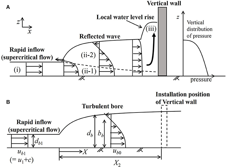
Figure 5. Kihara and Kaida (2016)'s interpretation of the relationship between the bore pressure and the flow property (A), and a conceptual diagram for applying the theory of Madsen and Svendsen (1983) to the physical model of bore pressure (B).

Based on the above-mentioned interpretation, Kihara and Kaida (2016) developed the semi-empirical physical model of bore pressure by using flow properties in a reflected wave. The high-velocity flow, which causes the hydrodynamic pressure for the momentum conversion at the front of the vertical wall, would be represented by the high-velocity flow inside the reflected wave at the vertical wall installation position in the condition where there is no vertical wall. In Kihara and Kaida (2016), by applying the theory of a turbulent bore that travels over the supercritical flow, proposed by Madsen and Svendsen (1983), the internal structure of the reflected wave is solved, and the flow properties inside the reflected wave at the vertical wall installation position in the condition where there is no vertical wall are obtained. That is, the reflected wave is regarded as a turbulent bore. Figure 5B shows a conceptual diagram for applying the theory of Madsen and Svendsen (1983).

The turbulent bore theory of Madsen and Svendsen (1983) is a theory that has been solved for a turbulent bore in which an inflow of the supercritical flow condition with vertically uniform velocity u_b1 and water depth d_b1 occurs. In this theory, the water depth d_b of the turbulent bore and the vertical distribution of the x-directional velocity inside the bore are predicted with a function of distance from the tip of the turbulent bore. The predicted velocity in the turbulent bore is the high velocity near the bed at the tip part of the turbulent bore, and it has a strong shear in the vertical direction. Moving toward the downstream side, the velocity distribution becomes uniform in the vertical direction. The vertical distribution of velocity u_b in the turbulent bore is given by the following equations:

$\begin{array}{cc}\begin{array}{l}{u}_b=u_{b0}+(u_{bs}-u_{b0})({-\sigma }_b^3+2{\sigma }_b^2)0\le {\sigma }_b\le 1\\ u_b=u_{b0}0<z\le a_b,\end{array}& (2)\end{array}$

where u_b0 is the velocity in the high velocity region, u_bs is the velocity at the water surface, z is the distance from the bed, σ_b = (z−a_b)(d_b−a_b), and a_b is the height of the bottom of the turbulent region in the turbulent bore.

The water depth and velocity distribution of the turbulent bore are calculated by inputting the water depth d_b1 and velocity u_b1 (or Froude number Fr_b1) of the inflow. By carrying out numerical integrations, the theoretical solution is obtained. Using the theoretical solution for Fr_b1 = 1.5, 2.0, 2.5, 3.0, 3.5, and 4.0, we develop the following approximation equations of the water depth d of the turbulent bore and the velocity u₀ in the high velocity region for Fr_b1 > 1.5 by applying least-square approach:

$\begin{array}{cc}\begin{array}{r}\frac{u_{b0}(X)}{u_{b1}}\approx 0.6+0.4\text{exp}\left\{-\left(\frac{3.2}{F{r}_{b1}^3}+0.02\right)\frac{X}{d_{b1}}\right\}\end{array}& (3)\end{array}$

$\begin{array}{cc}\begin{array}{r}\frac{d_b(X)}{d_{b1}}\approx 1+{\epsilon }_1\left\{1-exp(-{\epsilon }_2\frac{X}{d_{b1}})\right\}\end{array}& (4)\end{array}$

$\begin{array}{l}{\epsilon }_1=1.4(F{r}_{b1}-1)\end{array}$

$\begin{array}{l}{\epsilon }_2=\frac{2.5}{F{r}_{b1}\left\{F{r}_{b1}+min(1,\frac{F{r}_{b1}}{2.3})\right\}},\end{array}$

where X is the coordinate in the streamwise direction with its origin at the tip part of the turbulent bore. Near the tip part of the turbulent bore, although there is high-velocity flow in the x-direction at a low height, a flow toward the downstream occurs on the upper side. The flow converted to hydrodynamic pressure on the front of the vertical wall would be the flow at a height with a positive x-direction velocity. Inside the turbulent bore, The approximation equation of the height b_b with a positive x-direction velocity is obtained as:

$\begin{array}{cc}\begin{array}{r}\frac{b_b(X)}{d_{b1}}\approx min\left\{1+0.2\frac{X}{d_{b1}},\frac{d_b(X)}{d_{b1}}\right\}.\end{array}& (5)\end{array}$

To calculate the internal structure of the reflected wave at the installation position of the vertical wall under conditions where there is no vertical wall, it is necessary to predict the distance X₂ from the vertical wall installation position to the tip of the reflected wave. The distance from the vertical wall installation position to the tip of the reflected wave is predicted from the traveling speed c of the reflected wave using the following equation:

$\begin{array}{cc}\begin{array}{r}\frac{d{X}_2}{dt}=c.\end{array}& (6)\end{array}$

The positive direction of the traveling speed c is inverse with the positive x-direction. The theory of Madsen and Svendsen (1983) is for a stationary turbulent bore, and thus to apply it to a reflected wave moving to the upstream side, it is necessary to use a theory with respect to a coordinate system moving with the traveling speed c of the reflected wave. Therefore, the water depth d and velocity u in the quiescent conditions have the following relationship with the water depth d_b and velocity u_b in the moving coordinate system of the turbulent bore theory:

$\begin{array}{cc}\begin{array}{r}{d}_b=d,b_b=b,and{u}_b=u+c.\end{array}& (7)\end{array}$

The subscript b denotes a variable with respect to the coordinate system moving with the traveling speed c of the reflected wave. As can be seen from the experiment images in Figures 3C,D), after the reflected wave appears, it stays at the front of the vertical wall for about 3 s, and then travels to the upstream side. Times during which the reflected waves stay and traveling speeds c of the reflected wave, which are estimated from videos of the experiments, are also shown in Table 2.

TABLE 2

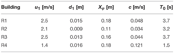
Table 2. Predicted characteristic water depth, velocity of inflow, traveling speed of reflected wave c, and duration of bore pressure T₀ for each case.

By solving equations (3–7) with inflow velocity and depth measured at V1 and H2 as the input conditions, the velocity u, water depth d, height with a positive x-direction velocity b at the vertical wall installation position in the condition, where there is no vertical wall, can be obtained. Here, we set minimum X₂ as 2 m, which was observed from the images of the experiments.

In bore pressure, both hydrodynamic pressure p_d and hydrostatic pressure p_s make a contribution, and thus bore pressure is assumed to be expressed as their sum.

$\begin{array}{cc}\begin{array}{r}p(z)=p_d(z)+p_s(z)\end{array}& (8)\end{array}$

The hydrodynamic pressure component p_d would have relationships with the velocity u₀(X₂) in the high-velocity region in the reflected wave at the vertical wall installation position (X = X₂), and with the height b(X₂) which has a positive x direction velocity, and is given as:

$\begin{array}{cc}\begin{array}{r}{p}_d(z)=\frac{1}{2}{\rho }_w{u_0(X_2)}^{2}f(z),\end{array}& (9)\end{array}$

where f (z) is the distribution function for the hydrodynamic pressure, and it is experimentally expressed with the following function type.

$\begin{array}{cc}\begin{array}{r}f(z)=1-{\left(\frac{z}{b(X_2)}\right)}^{4}z<b(X_2)\end{array}& (10)\end{array}$

$\begin{array}{l}f(z)=0z\ge b(X_2)\end{array}$

The hydrostatic pressure p_s is given as:

$\begin{array}{cc}\begin{array}{r}{p}_s(z)={\rho }_{w}g(b(X_2)-z)z<b(X_2)\end{array}& (11)\end{array}$

$\begin{array}{l}{p}_s(z)=0z\ge b(X_2).\end{array}$

Figure 6 compares the maximum value of wave pressure at each time measured in the experiment, and those predicted by the above-mentioned model. In Figure 6, bore pressure is predicted, limited to the conditions t' > 3U/g and Fr_b1 > 1.2, where t' denotes the time elapsed since the bore impacted the vertical wall. The former limitation is set because the bore pressure is defined as the pressure observed from the time when the water mass has shot up and fallen to the time when the pressure distribution becomes the hydrostatic form, and the time needed from impact of the bore with the structure until the water mass falls is given approximately by 3 U/g. The latter limitation is set because, in the turbulent bore theory, the inflow must be in the condition of supercritical flow. In the distribution form shown in Equations (10, 11), predicted wave pressure is maximum at z = 0 m. Figure 6 shows that experimental values are reproduced fairly well by the proposed model. The vertical distributions of predicted bore pressures over time of Figures 4C–E are compared with the measured pressures in Figure 7. The figure also shows good agreement among them.

FIGURE 6

Figure 6. Comparison of the maximum values of wave pressure at each time measured in the experiment (A) with the those predicted by the semi-empirical physical model (B).

FIGURE 7

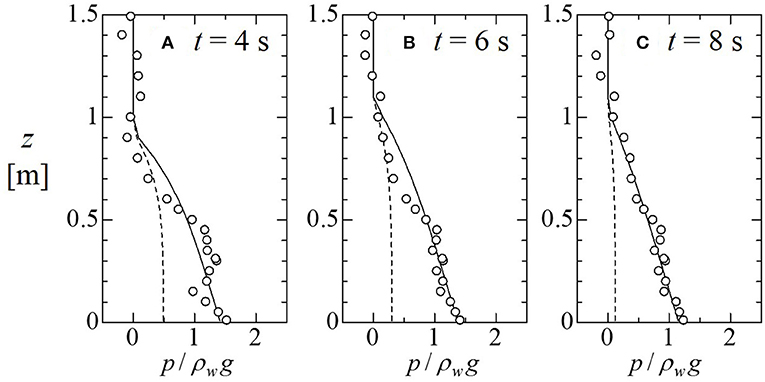
Figure 7. Comparison of the vertical distributions of predicted pressure for t = 4, 6, and 8 s to measured ones. Circles denote the measured pressure, solid lines denote the predicted pressure, and dashed lines denote the predicted hydrodynamic pressure. (A) t = 4 s, (B) t = 6 s, (C) t = 8 s.

Practical Application Method of Semi-empirical Physical Model of Bore Pressure

For prediction of bore pressure from the semi-empirical physical model mentioned in the previous section, it is necessary to input time-series of inundation depths and velocities of inflows, on which there are no effects of walls or structures, and lengths and traveling speed of reflected waves. However, the two-dimensional non-linear shallow water equation model (nSWE model) is often used for tsunami inundation simulations in practice (MLIT, 2012), and spatial and temporal distributions of depth-averaged velocity and water depth are calculated, but it is difficult to obtain the above-mentioned flow properties for bore pressure predictions from the simulations. In this section, we describe the method by which bore pressures are able to be predicted by the semi-empirical physical model with usage of numerical results of tsunami inundation simulations of the nSWE model.

Since it is not easy to use the numerical results of the tsunami inundation simulations of the nSWE model to directly predict the inflow properties for which there are no effects from walls or structures, or the lengths and traveling speed of reflected waves, it is rational to set characteristic values for them for predictions of bore pressures. First, at the moment of impact of a tsunami front on a target structure, velocities and water depths are spatially averaged in an upstream area of the structures. The spatial-averaged velocities and water depths are set as characteristic water depths and velocities of inflow.

Next, the characteristic parameter for determining the duration of bore pressure is modeled. As shown in Matsutomi (1991) and this study, vertical distribution of bore pressure is parabolic. This means that the hydrodynamic pressure p_d is greater than the hydrostatic pressure p_s in the duration of bore pressure. Time series distribution of p_d/p_s at the bed predicted in the previous section is shown in Figure 8A. Figure 8A shows that p_d/p_s at the bed is high just after the bore pressure starts to act, and becomes lower as the time has passed. When time has passed sufficiently, the hydrodynamic pressure becomes negligible, compared to the hydrostatic pressure, and the pressure pattern changes from bore pressure to quasi-steady-state pressure. Here, the duration of bore pressure is determined as the time from the bore pressure starts to act until p_d/p_s at the bed becomes sufficiently low. Strength of the hydrodynamic pressure would be related to the vertical gradient of streamwise velocity just near the vertical wall, a parameter representing the magnitude of the velocity gradient may be useful for the prediction of decrease of p_d/p_s. Thus, we show the time-series distribution of the following parameter, which represents the magnitude of velocity gradient in Figure 8B, and compares it to that of p_d / p_s at the bed, which is shown in Figure 8A.

$\begin{array}{cc}\begin{array}{r}\varphi =\frac{1}{u_{b0}}max\left[\frac{d{u}_b}{dz}\right].\end{array}& (12)\end{array}$

FIGURE 8

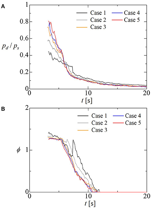
Figure 8. Time series distribution of predicted p_d / p_s at the bed (A) and φ (B).

When p_d/p_s is high, a different pattern is observed in between p_d/p_s and φ. On the other hand, when p_d/p_s decreases and becomes low in the range of 0.1–0.2, a similar pattern is observed among low p_d/p_s and φ. We focus attention on this similar pattern of p_d/p_s and φ in the range of p_d/p_s = 0.1–0.2, and we adopt φ as an indication of time from when p_d/p_s becomes a low value. Here, we define that pressure pattern changes from bore pressure to quasi-steady-state pressures when p_d/p_s becomes lower than 0.15. The comparison between Figures 8A,B shows that a value of φ corresponding to p_d/p_s = 0.15 is approximately 0.7. Thus, when φ becomes lower than 0.7, the pressure pattern would change from bore pressures to quasi-steady-state pressures.

By solving the theoretical solution of the turbulent bore theory of Madsen and Svendsen (1983), the relationship between φ and distance X₂ from the tip of the reflected wave to the structure for various Froude numbers is investigated, and an approximation equation of the distance X_φ corresponding to φ = 0.7 is built as follows:

$\begin{array}{cc}\begin{array}{r}\frac{X_{\varphi }}{d_{b1}}\approx 12-exp\left\{-1.2(F{r}_{b1}-3.1)\right\}.\end{array}& (13)\end{array}$

Pressure pattern changes from bore pressure to quasi-steady-state pressures, when the length of the reflected wave X₂ becomes longer than X_φ, and X_φ is considered as the parameter related to duration of bore pressure in this study.

Next, the characteristic traveling speed of a reflected wave is obtained as follows. As described in Ikeya et al. (2015), traveling speeds of reflected waves from structures are affected by blockings due to the structures in flow channels. As the blocking ratio increases, the traveling speeds increases. This is caused by effects of blocking ratio on flow rates through and around target structures. Ikeya et al. (2015) describe that there is a critical depth at the position of a structure since an inflow at the front of the structure is in the condition of subcritical flow and a flow just behind the structure is in the condition of supercritical flow, and proposed the relationship between flow rate of inflow and flow at the position of the structure under conditions where there is no structures as follows:

$\begin{array}{cc}\begin{array}{r}\frac{d\overline{u}}{d_1{u}_1}=min\left[1,\frac{(1-\gamma )C_c}{F{r}_1}{\left(\frac{2}{3}\frac{h_f}{d_1}\right)}^{3/2}\right],\end{array}& (14)\end{array}$

where d₁, d₁, and Fr₁ are the water depth, velocity, and the Froude number of an inflow, respectively, as well as the definition of the previous section, d, $\overline{u}$, and h_f are the water depth, depth-averaged velocity, and the specific energy at the position of the structure under conditions where there are no structures, γ is the blocking ratio, and C_c is the contraction coefficient [= 0.6, following Ikeya et al. (2015)]. The specific energy h_f at the position of the structure under conditions where there is no structure is given as

$\begin{array}{cc}\begin{array}{r}{h}_f=\frac{{\overline{u}}^2}{2g}+d.\end{array}& (15)\end{array}$

The mass conservation equation in the coordinate system moving with the traveling speed c of the reflected wave is given as

$\begin{array}{cc}\begin{array}{r}(u_1+c)d_1=(\overline{u}+c)d.\end{array}& (16)\end{array}$

By solving equations (14–16) together with equations (4, 6, 7) for inflow properties d₁ and u₁, we can calculate the time evolutions of the distance X₂ from the tip of the reflected wave to the structure or the wall and the traveling speed c (≥ 0) of the reflected wave. As the initial conditions, we set a minimum value of X₂ at t = 3 u₁/g. Although there is no solid physical basis of setting of the minimum X_2min, X_2min would be related to the strength of the inflow. Thus, we set

$\begin{array}{cc}\begin{array}{r}{X}_{2min}=\frac{{u_1}^2}{2g}+d_1.\end{array}& (17)\end{array}$

In the previous section, we set X_2min as 2 m, which was determined by the images of the experiments, and the value is harmonic with equation (17).

The time evolution of non-dimensional traveling speed (c/(gd₁)^1/2) of the reflected wave in the condition of the blocking ratio γ = 0.25 is shown in Figure 9. In the figure, the non-dimensional traveling speeds for Fr₁ = 2 and 3, and d₁ = 0.2, 0.6, and 1.0 are shown, respectively. The figure shows that the non-dimensional traveling speed (c/(gd₁)^1/2) depends on the Froude number of inflow Fr₁. As the time elapses, the non-dimensional traveling speeds approach constant values c₀ depending on Fr₁. In this study, the constant values c₀ are set as the characteristic value of the traveling speed c, and the time T₀ when the length of the reflected wave X₂ becomes X_φ, is calculated from

$\begin{array}{cc}\begin{array}{r}{T}_0=\frac{X_{\varphi }}{c_0}.\end{array}& (18)\end{array}$

FIGURE 9

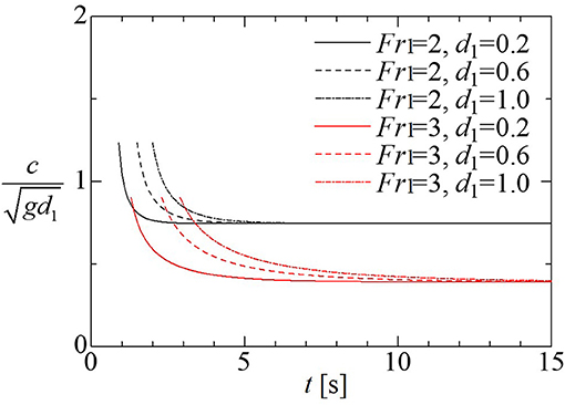
Figure 9. Time evolution of non-dimensional traveling speed (c /(gd₁)^1/2) of the reflected wave in the condition of the blocking ratio γ = 0.25 for Fr₁ = 2 and 3, and d₁ = 0.2, 0.6, and 1.0.

The relationship between T₀ and Fr₁ in the conditions of γ = 0.25 and 1 are obtained by using equation (13) and the relationship between c₀ and Fr₁, and approximately expressed as

$\begin{array}{cc}\begin{array}{r}{T}_0\approx 20{(F{r}_1-1)}^2\frac{d_1}{u_1},\end{array}& (19)\end{array}$

and

$\begin{array}{cc}\begin{array}{r}{T}_0\approx 18(F{r}_1-1.3)\frac{d_1}{u_1},\end{array}& (20)\end{array}$

respectively. The time T₀ is the duration of bore pressure. The characteristic value of the traveling speed c₀ is calculated from equations (13, 18), and (19) or (20).

Finally, it is necessary to obtain u₀ (X₂). Tsunami inundation simulations of the nSWE model predict the depth-averaged velocity $\overline{u}(X_2)$, and thus, we convert $\overline{u}(X_2)$ into u₀ (X₂). From equation (2) in the theory of Madsen and Svendsen (1983), the relationship between $\overline{u}(X_2)$ and u₀ (X₂) is expressed as

$\begin{array}{cc}\begin{array}{l}\overline{u_b}d={\displaystyle {\int }_0^{a_b}{u}_{b0}dz}+{\displaystyle {\int }_{a_b}^d{u}_{b0}+\left(u_{bs}-u_{b0}\right)\left(-{\sigma }_b^3+2{\sigma }_b^2\right)dz}\\ =u_{b0}d+\left(u_{bs}-u_{b0}\right){\displaystyle {\int }_{a_b}^d\left(-{\sigma }_b^3+2{\sigma }_b^2\right)dz}\\ =u_{b0}d+\left(u_{bs}-u_{b0}\right)\left(d-a_b\right){\displaystyle {\int }_0^1\left(-{\sigma }_b^3+2{\sigma }_b^2\right)d}\sigma \\ =u_{b0}d+u_{b0}\Gamma B{S}_1\\ \iff u_0\left(X_2\right)=\frac{\left(\overline{u}+c\right)d\left(X_2\right)}{d\left(X_2\right)+\Gamma B{S}_1}-c,\end{array}& (21)\end{array}$

where $\text{Γ}=\frac{u_{bs}-u_{b0}}{u_{b0}},B=(d-a_b)$, and $S_1=\underset{0}{\overset{1}{\int }}-{{\sigma }_b}^3+2{{\sigma }_b}^{2}d\sigma .$

From the theoretical solution, Γ and B are obtained as a function of X₂, and the relationships are approximately expressed as

$\begin{array}{l}\text{Γ}\approx \min \left({\text{Γ}}_1,{\text{Γ}}_2\right){\gamma }_2\ge -1.5\\ \text{Γ}\approx \max \left({\text{Γ}}_1,{\text{Γ}}_2\right){\gamma }_2<-1.5\\ {\text{Γ}}_1=-1.5\exp \left(-\frac{1}{{\gamma }_1}\frac{X_2}{d_1}\right)\\ {\text{Γ}}_2={\gamma }_2\exp \left[-0.1{\left(\frac{X_2}{d_1}\right)}^{{\gamma }_3}\right]\\ {\gamma }_1=8{\left(F{r}_1-0.9\right)}^2\\ {\gamma }_2=1-3.2lnF{r}_1\\ {\gamma }_3=0.93-0.045F{r}_1,\\ and\\ \frac{B}{d_1}=\min \left(-\frac{B_0}{d_1},\frac{d}{d_1}\right)\\ \frac{B_0}{d_1}\approx 0.65\frac{X_2}{d_1}\exp \left(-\frac{1}{B_1}\frac{X_2}{d_1}\right)\frac{X_2}{d_1}\le \frac{1}{2}{B}_1\\ \frac{B_0}{d_1}\approx B_2\left(\frac{X_2}{d_1}-\frac{1}{2}{B}_1\right)+0.2B_1\frac{X_2}{d_1}>\frac{1}{2}{B}_1\\ B_1=3F{r}_1{}^2-1.5F{r}_1-1.5\\ B_2=0.055F{r}_1+\mathrm{0.015.}\end{array}$

By using the above-mentioned settings and equations, bore pressures acting on a structure are predicted with usage of the numerical results of tsunami inundation simulations of the nSWE model as follows:

(i) By spatially averaging velocities and water depths in an upstream area of the structure at the moment of impact from a tsunami front on the structure, the characteristic water depths and velocities of the inflow are obtained. Then, the characteristic Froude number of the inflow is determined.

(ii) From equations (13, 19, 20), X_φ, and the duration of bore pressure T₀ are calculated, respectively.

(iii) The characteristic value of the traveling speed c₀ is calculated from equation (18).

(iv) After the impact of the tsunami front, the time evolution of distance X₂ from the tip of the reflected wave to the structure is calculated from equation (15). In the calculation, the characteristic traveling speed c₀ is used as c.

(v) u₀ (X₂) for each time is calculated from equation (21) with $\overline{u}$ and d for each time, which are calculated by tsunami inundation simulations of the nSWE model. In these calculations, the characteristic water depth and Froude number of inflow calculated step (i) is used as d₁ and Fr₁. Furthermore, the water depth in front of the structure evaluated in the tsunami inundation simulations is used as d_b(X₂) in equation (5).

(vi) Bore pressures at each time are calculated from equations (8–11) until time from the impact of the tsunami front is longer than T₀. Here, inundation depth d for each time, which is calculated by tsunami inundation simulations of the nSWE model is used as b(X₂) in (10, 11) for simplicity and conservativeness.

It should be noted that if we can obtain X₂ and c₀ of the reflected wave directly from the numerical results of nSWE model by tracking the front of the reflected wave, procedures (iii) and (iv) can be passed.

In the above-mentioned procedure for predictions of bore pressures by using the proposed physical model, there are no iterative calculations. Furthermore, time series of inflow conditions, which have no effect on buildings are not needed as input parameters of the physical model. Thus, the issues in the physical model proposed by Kihara and Kaida (2016) on practical uses are solved.

Application of Semi-empirical Physical Model to an Inundation Simulation

Method

In this section, we show an application of the proposed semi-empirical model of bore pressure described in the previous section to evaluations of pressures on buildings in a tsunami inundation area. To do that, we carry out two kinds of inundation simulations, and compare pressures predicted by both simulations. The first is a three-dimensional non-hydrostatic simulation, and pressures on buildings are directly predicted by the simulation. The open source computational fluid dynamics library OpenFOAM, that have been used for evaluations of wave pressures on coastal structures, and its applicability have been shown by some studies (e.g., Hayatdavoodi et al., 2014; Higuera et al., 2014; Douglas and Nistor, 2015; Sarjamee et al., 2017a,b), is used for the three-dimensional non-hydrostatic simulation. The second is the two-dimensional simulation by an nSWE model, and pressures on buildings are not directly predicted, and thus predicted by inputting the numerical result in the semi-empirical model of bore pressure.

Inundation simulations of a benchmark case are carried out. The benchmark case is the tsunami inundation experiment carried out at Oregon State University, and details of the experiment are found in (Rueben et al., 2011) and Park et al. (2013). The plan and elevation views of their experiment can be referred to Figure 2 of Park et al. (2013). The experiment was carried out by using a rectangular basin that was 40.0 m long, 26.5 m wide, and 2.1 m deep. A tsunami wave was generated by a piston-type wavemaker. The topography of the town of Seaside, Oregon, was ideally constructed at 1:50 scale, with a smooth concrete face. The bathymetry consisted of 10 m horizontal section near the wavemaker with a depth of 0.97 m, an 8 m section with a slope of 1:15, a 15 m section with a slope of 1:30, and an inundation section, which is horizontal. On the inundation section, many buildings were set. The water levels measured 2.086 m from the wavemaker was used as the boundary condition in numerical simulations.

The pressures on the buildings R1, R2, R3, and R4 in the inundation area, which are shown in Figure 10, are evaluated by the above-mentioned two approaches. For the three-dimensional non-hydrostatic simulation of OpenFOAM, the interFoam solver, which is a two-phase and incompressible fluid solver, was used. In the solver, continuity and Reynolds-averaged Navier-Stokes equations for both the water and air phases are solved. The k-ε SST model was used for the turbulent model. At the bed and building faces, logarithmic-law over the smooth surface was adopted as the boundary condition. The grid resolution was variant in space, and the resolution on the land area was set as 0.018 m in the horizontal direction and 0.009 m in the vertical direction. The grid resolution near the wavemaker was most coarse, and was set as 0.5 m in the streamwise direction, 0.4 m in the spanwise direction, and 0.009 m in the vertical direction. The total grid number was 20,000,000. For the numerical simulation, a parallel computation with 256 cores with a multi-core processor Intel Xeon CPU (E5-2670, 2.6 GHz) was carried out, and it took 6.5 h for the time-integration for 30 s.

FIGURE 10

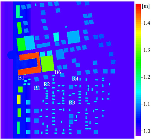
Figure 10. Elevation of topography in the inundation area. Positions of buildings R1, R2, R3, and R4 are depicted.

In the nSWE model, a depth-averaged momentum conservation equation and a mass conservation equation are solved, and depth-averaged velocities and inundation depths are calculated by inundation simulations. The hydrostatic assumption is applied in the depth-averaged momentum conservation equation, and thus the pressures on a building are not able to be evaluated directly from inundation simulations by the nSWE model. Thus, for evaluations of tsunami pressures on buildings, it is necessary to couple the inundation simulations by the nSWE model with semi-empirical physical model of bore pressures. The nSWE model used in this study adopt the staggered grid arrangement, and thus, the momentum conservation equation is solved on cell faces and the mass conservation equation is solved at cell centers. This means that the scalar variables are stored at cell centers, whereas momentum or velocity are stored at cell faces. The Manning coefficient was set as 0.005 m^−1/3. The grid resolution was variant in space, and the resolution on the land area was set as 0.02 m. The grid resolution near the wavemaker was most coarse, and was set as 0.05 m. The total grid number was 1,552,672. For the numerical simulation, a single computation with a multi-core processor Intel Xeon CPU (E5-2450 2.10 GHz) was carried out, and it took 45 h for the time-integration for 30 s. The CPU time for the simulation of the nSWE model was much lower than that for the simulation of the three-dimensional non-hydrostatic simulation of OpenFOAM.

Numerical Results

Comparison of Flow Properties

The water depths and velocities in the streamwise direction at measurement points B1 and B6 predicted by both simulations are compared to the experimental data in Figure 11. The locations of the measurement points B1 and B2 are depicted in Figure 10. The time of numerical results were corrected by comparisons of water levels at WG3, which was located at 18.618 m from the wavemaker and whose location can be referred to Figure 2 of Park et al. (2013), between experimental and numerical results. The figure shows rough agreement between the numerical results and experimental data. It should be noted that the confirmations of good agreement in comparisons among the numerical results are important in this study since the pressure or force on buildings were not measured in the experiment, and the comparisons of the pressure or force on buildings predicted by both numerical approaches are materials of the discussions in this study.

FIGURE 11

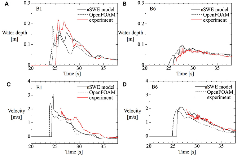
Figure 11. Comparisons of water depths and x-directional velocities at B1 and B6 between by the laboratory experiment, the three-dimensional simulation of OpenFOAM, and the two-dimensional simulation of nSWE model. (A) water depth at B1, (B) water depth at B6, (C) velocity at B1, and (D) velocity at B6.

Wave Pressure Predicted by Three-Dimensional Non-hydrostatic Simulation

First, the tsunami wave forces acting on the seaward side of buildings R1, R2, R3, and R4 are calculated by integrating pressures on the surface predicted by the three-dimensional simulation of OpenFOAM, and are shown in Figure 12A. At buildings R1 and R2, which are located near the coast, the maximum forces are observed approximately after 1 s has passed since the tsunami impacted the buildings. On the other hand, at buildings R3 and R4, which are located farther from the coast than R1 and R2, the maximum forces are observed after 4 s or more have passed since the tsunami impacted the buildings R3 and R4, and the maximum forces are lower than those of R1 and R2. As shown in Figure 11, the comparison of inundation depth and velocity at B6 and B1 shows that the inundation depth and the specific energy become lower as the distance from coastal line increases, resulting in the tsunami wave force being lower, as mentioned by our early studies (Kihara et al., 2012; Takabatake et al., 2013).

FIGURE 12

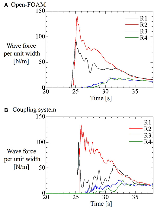
Figure 12. Tsunami wave forces acting on the seaward side of buildings R1, R2, R3, and R4 predicted by the three-dimensional simulation of OpenFOAM (A), and the coupling system of the semi-empirical physical model and the two-dimensional simulation of nSWE model (B).

The vertical distributions of pressure head at the center line of the seaward side of the buildings R1, R2, R3, and R4 when maximum wave forces were observed, are shown in Figure 13. At the buildings R1 and R2, whose maximum forces were observed approximately after 1 s have passed since the tsunami impacted the buildings, the vertical distribution of the pressure is not the hydrostatic form. This means that the maximum force occurred when the bore pressure is dominant. On the other hand, at buildings R3 and R4, whose maximum forces are observed after 4 s or more have passed since the tsunami impacted the buildings R3 and R4, the vertical distribution of the pressure is the hydrostatic form. This means that the maximum force occurred when the quasi-steady-state pressure is dominant.

FIGURE 13

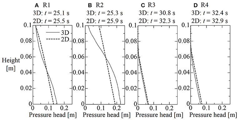
Figure 13. The vertical distributions of pressure head at the center line of the seaward side of buildings R1, R2, R3, and R4, which are predicted by the three-dimensional simulation of Open-FOAM (3D) and predicted by the coupling system of the semi-empirical physical model and the two-dimensional simulation of nSWE model (2D), when maximum wave forces were observed. Time when the maximum wave forces were observed are also described. (A) R1, (B) R2, (C) R3, and (D) R4.

Wave Pressure Predicted by Semi-empirical Physical Model of Bore Pressure

Next, by using the numerical result of the two-dimensional simulation of the nSWE model, we predict pressure distribution on the buildings from the semi-empirical physical model of bore pressure. In this study, the staggered grid arrangement was adopted, and velocities are calculated at cell faces where the momentum conservation equation is solved. On the other hand, water depths are calculated at cell centers where the mass conservation equation is solved. Since hydrodynamic pressure is strongly related to the momentum transfer process, the velocities stored at points where the momentum conservation equation is solved are preferred to be used for the prediction of hydrodynamic pressure. Thus, the velocity $\overline{u}(i)$ stored at a cell face next to a cell of building, and the averaged value ((d (i- 1/2) + d (i + 1/2))/2) of the inundation depths stored at the cell centers, which are the neighbors of the cell face, are used.

As written in step (i), the spatially averaged velocities and water depths are obtained. The averages are done over the wet bed in rectangular areas with 0.5 m in the streamwise direction and 0.9 m in the spanwise direction in the seaward side of the buildings. The length of the rectangular area in the streamwise direction was similar in length to the width of the buildings. In step (ii), the duration of bore pressure T₀ is calculated from equation (19) or (20). In this calculation, the blockage ratio is needed, although the blockage ratio depends on flow directions and, thus, it is not easy to determine blockage ratio accurately. In this simulation condition, the flow path is partially blocked, and thus equation (16), which is the approximation equation for the blockage ratio of 0.25, is used. Although the blockage ratio is not exactly equal to 0.25 in the simulation condition, the inaccuracy of the blockage ratio may be not important, considering rough accuracy of this semi-empirical model. The predicted characteristic water depths, velocities of inflows, traveling speeds of reflected waves c, and duration of bore pressure T₀ are shown in Table 2. As shown in Table 2, in the cases of buildings R1 and R2, the duration of bore pressure is longer than the time of occurrence of maximum forces since the tsunami impacted the buildings in the numerical results of the three-dimensional simulation. On the other hand, in the cases of buildings R3 and R4, the duration of bore pressure is shorter than the time of occurrence of maximum forces since the tsunami impacted the buildings. This means that at buildings R1 and R2, the maximum forces occurred when the bore pressure is dominant, and on the other hand, that at buildings R3 and R4 the maximum forces occurred when the quasi-steady-state pressure is dominant. This result is harmonic with the results of the three-dimensional simulation.

The tsunami wave forces that acted on the seaward side of buildings R1, R2, R3, and R4 are calculated by integrating pressures on the surface predicted by the coupling system of the semi-empirical physical model of bore pressure and the two-dimensional simulation of the nSWE model, and are shown in Figure 12B. Here, for reference, pressures after the duration of the bore pressure are predicted by the evaluation method of quasi-steady-state pressure, which was proposed by early studies of authors (Kihara et al., 2012; Takabatake et al., 2013).

$\begin{array}{cc}\begin{array}{r}p(z)={\rho }_{w}g(d+\frac{{\overline{u}}^2}{2g}-z)z<d+\frac{{\overline{u}}^2}{2g}\end{array}& (22)\end{array}$

$\begin{array}{l}p(z)=0z\ge d+\frac{{\overline{u}}^2}{2g},\end{array}$

Figure 12B shows that maximum forces are observed approximately 1 s after the tsunami impacted buildings R1 and R2. However, at buildings R3 and R4, maximum forces are observed after 4 s or more have passed since the tsunami impacted the building. These results agree with those of the three-dimensional simulation.

The vertical distributions of pressure head at the center line of the seaward side of the buildings R1, R2, R3, and R4 predicted by the coupling system when maximum wave forces were observed are shown in Figure 13. At buildings R1 and R2, whose maximum forces were observed approximately after 1 s have passed since the tsunami impacted the buildings, the pressure distributions are predicted by the semi-empirical physical model of bore pressure. On the other hand, at the buildings R3 and R4, whose maximum forces are observed after 4 s or more have passed since the tsunami impacted buildings R3 and R4, the vertical distributions of the pressures are predicted by equation (22). Compared to the numerical results of the three-dimensional simulation, the pressure at buildings R1 and R2 predicted by the coupling system distributes more linearly. However, the wave forces and the magnitude of pressure predicted by the coupling system roughly agree with those of the three-dimensional simulation. Thus, we think that the proposed semi-empirical model has acceptable accuracy for engineering applications.

Conclusions

In this study, based on the results of the large-scale hydraulic experiment focused on the bore pressure by Kihara and Kaida (2016), relationships between flow profiles and bore pressure were investigated. Immediately after a bore impacted the vertical wall, an impulsive pressure was observed. After that, a water column was observed, but non-negligible positive wave pressure acted at a lower height than the height of the top of the water column. After the water column collapsed, a reflected wave was generated from the vertical wall to the upstream side. Although a local rise was observed in the water surface just in front of the vertical wall, positive pressure acts at a lower height than the height of the local rise of the water surface. The distribution form of the wave pressure at this time was parabolic. As the front of the reflected wave moved away from the vertical wall, the pressure distribution approached the hydrostatic form.

By considering the relationships between the flow profiles and the bore pressure, a semi-empirical physical model of bore pressure was developed based on the interpretation of Kihara and Kaida (2016). By applying the theory of a turbulent bore, proposed by Madsen and Svendsen (1983), a set of approximation equations for solving the internal structure of the reflected wave was presented. Since the hydrodynamic pressure at the front of the vertical wall would play a role in the conversion of the momentum of the flow in the streamwise direction into that in the vertical direction, the hydrodynamic pressure in the bore pressure was modeled as a function of velocity inside the reflected wave at the vertical wall installation position in the condition where there is no vertical wall, which can be obtained by the approximation equations. Comparisons of predicted pressure by the semi-empirical physical model to the measured one showed good agreement.

Also, we presented an application method and procedure of the semi-empirical physical model to evaluations of bore pressure with usage of numerical results of two-dimensional simulations of tsunami inundation by the nSWE model.

Finally, we applied the semi-empirical physical model to evaluations of pressures on buildings in an inundation area. To do that, we carried out tsunami inundation simulations by both a three-dimensional non-hydrostatic simulation by OpenFOAM and a two-dimensional simulation by an nSWE model. Pressures on buildings in an inundation area predicted by the coupling system of the semi-empirical physical model and the numerical results of two-dimensional simulation with those predicted directly by the three-dimensional simulation were compared. The comparison shows that bore pressure predicted by the coupling system distributes more linearly than that predicted by the three-dimensional simulation. However, the wave forces and the magnitude of pressure predicted by the coupling system roughly agreed with those of the three-dimensional simulation. While refinement of the semi-empirical physical model for improvement of accuracy is still needed, the proposed semi-empirical model would have acceptable accuracy for engineering applications.

Bore pressures on buildings can be evaluated well by carrying out three-dimensional hydrodynamic simulations. However, it needs very expensive numerical costs for solving wide inundation areas of actual tsunamis by three-dimensional numerical simulations to predict bore pressures in good accuracy. Also in this study, the CPU time for the simulation of the nSWE model was much lower than that for the simulation of the three-dimensional non-hydrostatic simulation of OpenFOAM. Thus, the coupling system of the semi-empirical physical model and the numerical results of two-dimensional simulation would be useful for predictions of bore pressures in wide inundation areas.

Author Contributions

NK developed the model of bore pressure and wrote the manuscript. HK carried out the experiment.

Conflict of Interest Statement

The authors declare that the research was conducted in the absence of any commercial or financial relationships that could be construed as a potential conflict of interest.

References

Al-Faesly, T., Palermo, D., Nistor, I., and Cornett, A. (2012). Experimental modeling of extreme hydrodynamic forces on structural models. Int. J. Protect. Struct. 3, 477–505. doi: 10.1260/2041-4196.3.4.477

CrossRef Full Text | Google Scholar

Arikawa, T., Ikebe, M., Yamada, F., Shimosako, K., and Imamura, F. (2005). Large model test of tsunami force on a revetment and on a land structure. Ann. J. Coast. Eng. JSCE 52, 746–750. doi: 10.9753/icce.v34.structures.44

CrossRef Full Text | Google Scholar

Arikawa, T., Ohtubo, D., Nakano, F., Shimosako, K., Takahashi, S., Imamura, F., et al. (2006). Large model test on surge front tsunami force. Ann. J. Coast. Eng. JSCE 53, 796–800. doi: 10.2208/proce1989.54.846

CrossRef Full Text | Google Scholar

Cross, R. H. (1967). Tsunami surge forces. J. waterw. Harb. Div. 93, 201–234.

Google Scholar

Douglas, S., and Nistor, I. (2015). On the effect of bed condition on the development of tsunami-induced loading on structures using OpenFOAM. Nat. Hazar. 76, 1335–1356. doi: 10.1007/s11069-014-1552-2

CrossRef Full Text | Google Scholar

Fukui, Y., Nakamura, M., Shiraishi, H., and Sasaki, Y. (1963). Hydraulic study on tsunami. Coast. Eng. Japan 6, 67–82. doi: 10.1080/05785634.1963.11924633

CrossRef Full Text | Google Scholar

Hayatdavoodi, M., Seiffert, B., and Ertekin, R. C. (2014). Experiments and computations of solitary-wave forces on a coastal-bridge deck. Part II: deck with girders. Coast. Eng., 88, 210–228. doi: 10.1016/j.coastaleng.2014.02.007

CrossRef Full Text | Google Scholar

Higuera, P., Lara, J. L., and Losada, I. J. (2014). Three-dimensional interaction of waves and porous coastal structures using OpenFOAM®. Part I: formulation and validation. Coast. Eng. 83, 243–258. doi: 10.1016/j.coastaleng.2013.08.010

CrossRef Full Text | Google Scholar

Ikeya, T., Suenaga, S., Fukuyama, T., Akiyama, Y., Suzuki, N., and Tateno, T. (2015). Evaluation method of tsunami wave force acting on land structures considering reflection properties. J. JSCE, Ser. B2 (Coast. Eng.) 71, 985–990. doi: 10.2208/kaigan.71.I_985

CrossRef Full Text | Google Scholar

Kihara, N. (2016). Large-scale tsunami physical simulator - a new type of experimental flume for research on tsunami impact. Hydrolink, IAHR 1, 24–25.

Google Scholar

Kihara, N., and Kaida, H. (2016). On evaluation of tsunami bore pressure on a vertical wall. J. JSCE Ser. B2 72, 973–978. doi: 10.2208/kaigan.72.I_973

CrossRef Full Text | Google Scholar

Kihara, N., Niida, Y., Takabatake, D., Kaida, H., Shibayama, A., and Miyagawa, Y. (2015). Large-scale experiments on tsunami-induced pressure on a vertical tide wall. Coast. Eng. 99, 46–63. doi: 10.1016/j.coastaleng.2015.02.009

CrossRef Full Text | Google Scholar

Kihara, N., Takabatake, D., Yoshii, T., Ikeno, M., Ota, K., and Tanaka, N. (2012). Tsunami Fluid Force on Land Structures (Part I) - Numerical Study for Structures With Finite Width Under Non-Overflow Condition-. CRIEPI Res. Report N12010.

Madsen, P. A., and Svendsen, I. A. (1983). Turbulent bores and hydraulic jumps. J. Fluid Mech. 129, 1–25. doi: 10.1017/S0022112083000622

CrossRef Full Text | Google Scholar

Matsutomi, H. (1991). The pressure distribution and the total wave force. Coast. Eng. Japan 38, 626–640.

Google Scholar

MLIT (2012). Guide to Determining the Potential Tsunami Inundation (Version 2.00). Seacoast Office, Water and Disaster Management Bureau, Ministry of Land, Infrastructure, Ministry of Land, Infrastructure, Transport and Tourism.

Nouri, Y., Nistor, I., Palermo, D., and Cornett, A. (2010). Experimental investigation of tsunami impact on free standing structures. Coast. Eng. J. 52, 43–70. doi: 10.1142/S0578563410002117

CrossRef Full Text | Google Scholar

Palermo, D., Nistor, I., Al-Faesly, T., and Cornett, A. (2013). Impact of tsunami forces on structures. J. Tsunami Soc. Int. 32, 2, 58–76.

Google Scholar

Park, H., Cox, D. T., Lynett, P. J., Wiebe, D. M., and Shin, S. (2013). Tsunami inundation modeling in constructed environments: a physical and numerical comparison of free-surface elevation, velocity, and momentum flux. Coast. Eng. 79, 9–21. doi: 10.1016/j.coastaleng.2013.04.002

CrossRef Full Text | Google Scholar

Ramsden, J. D. (1996). Forces on a vertical wall due to long waves, bores, and dry-bed surges. J. Wwaterw. Port Coast. Ocean Eng. 122, 134–141. doi: 10.1061/(ASCE)0733-950X(1996)122:3(134)

CrossRef Full Text | Google Scholar

Ramsden, J. D., and Raichlen, F. (1990). Forces on vertical wall caused by incident bores. J. Waterw. Port Coast. Ocean Eng. 116, 592–613. doi: 10.1061/(ASCE)0733-950X(1990)116:5(592)

CrossRef Full Text | Google Scholar

Rueben, M., Holman, R., Cox, D., Shin, S., Killian, J., and Stanley, J. (2011). Optical measurements of tsunami inundation through an urban waterfront modeled in a large-scale laboratory basin. Coas. Eng. 58, 229–238. doi: 10.1016/j.coastaleng.2010.10.005

CrossRef Full Text | Google Scholar

Sarjamee, S., Nistor, I., and Mohammadian, A. (2017a). Large eddy simulation of extreme hydrodynamic forces on structures with mitigation walls using OpenFOAM. Nat. Hazar. 85, 1689–1707. doi: 10.1007/s11069-016-2658-5

CrossRef Full Text | Google Scholar

Sarjamee, S., Nistor, I., and Mohammadian, A. (2017b). Numerical investigation of the influence of extreme hydrodynamic forces on the geometry of structures using OpenFOAM. Nat. Hazar. 87, 213–235. doi: 10.1007/s11069-017-2760-3

CrossRef Full Text | Google Scholar

Stansby, P. K., Chegini, A., and Barnes, T. C. D. (1998). The initial stages of dam-break flow. J. Fluid Mech. 374, 407–424. doi: 10.1017/S0022112098009975

CrossRef Full Text | Google Scholar

St-Germain, P., Nistor, I., Townsend, R., and Shibayama, T. (2013). Smoothed-particle hydrodynamics numerical modeling of structures impacted by tsunami bores. J. Waterway Port Coast. Ocean Eng. 140, 66–81. doi: 10.1061/(ASCE)WW.1943-5460.0000225

CrossRef Full Text | Google Scholar

Stoker, J. J. (2011). Water Waves: The Mathematical Theory With Applications, Vol 36. New York, NY: John Wiley & Sons.

Google Scholar

Takabatake, D., Kihara, N., and Tanaka, N. (2013). Numerical study for the hydrodynamic pressure on the front of onshore structures by tsunami. J. JSCE Ser. B2 69, 851–855. doi: 10.2208/kaigan.69.I_851

CrossRef Full Text | Google Scholar

Wei, Z., Dalrymple, R. A., Hérault, A., Bilotta, G., Rustico, E., and Yeh, H. (2015). SPH modeling of dynamic impact of tsunami bore on bridge piers. Coast. Eng. 104, 26–42. doi: 10.1016/j.coastaleng.2015.06.008

CrossRef Full Text | Google Scholar