A Kernel-Based Method for Modeling Non-harmonic Periodic Phenomena in Bayesian Dynamic Linear Models

1. Introduction

In civil engineering, Structural Health Monitoring (SHM) is a field of study that aims at monitoring the state of a civil structure based on time series data. One key aspect of SHM is to detect anomalies from the analysis of structural responses, including—but not limited to—displacement, velocity, acceleration, and strain measurements collected over time using, for example, laser displacement sensors, velocimeters, accelerometers, or strain gauges. Monitoring operates under real field conditions and, therefore, SHM must deal with observations collected at irregular time intervals, missing values, high noise level, sensor drift, and outliers (Goulet and Koo, 2018).

One applicable approach for SHM time series analysis and forecasting is to decompose the observed structural response into a set of generic components including baseline, periodic, and residual components (Léger and Leclerc, 2007; Goulet and Koo, 2018). The baseline component captures the baseline response of a civil structure, which is directly related to the irreversible changes due to the aging of a structure over time. The periodic components model the periodic reversible changes due to the influence of external effects such as temperature, humidity, pressure, and traffic load. The residual component takes into account the modeling error. Each component is associated with a set of unknown model parameters which needs to be learned from a training dataset.

Periodicity in time series data is very common. Periodicity is of major importance in SHM because the changes in magnitude of the periodic pattern due to external effects are usually much larger than the magnitude of irreversible changes related to the health of the structure. It is worth mentioning that modeling external effects, when they are observed, is of major importance. Therefore, modeling periodic phenomena with accuracy is crucial to detect abnormal behavior in structural responses. The periodicity observed in structural responses have many origins: (i) annual cycles due to the seasons, (ii) daily cycles due to the day/night alternance, and (iii) hourly, weekly, and yearly cycles due to working days, weekends, and holidays (Goulet and Koo, 2018). In this paper, the terms periodicity (period), seasonality (season), and cyclicity (cycle) are used interchangeably whether or not the observed periodic patterns are related to well-known seasons. Periodic patterns found in SHM time series data may exhibit simple harmonic patterns, in the sense that they can be modeled using a single sinusoidal function. This is often the case for the effects induced by the daily and yearly air temperature variation. However, other periodic patterns are more complex. They are usually referred to as non-harmonic patterns because they cannot be modeled by a single sinusoidal function. For instance, in the field of dam engineering, the ambient air and water reservoir contribute to the establishment of a thermal gradient through the structure, which leads to a periodic non-harmonic pattern on the observed displacements time series (Léger and Leclerc, 2007; Tatin et al., 2015; Salazar and Toledo, 2018). In bridge monitoring, the effects related to traffic load variations generally display a non-harmonic weekly periodic pattern due to the day/night as well as the weekdays/weekend alternance (Westgate et al., 2015; Goulet and Koo, 2018).

Regression techniques, such as multiple linear regression (Léger and Leclerc, 2007; Tatin et al., 2015; Gamse and Oberguggenberger, 2017) and artificial neural networks (Mata, 2011), are widely used to perform time series decomposition in SHM. In the multiple linear regression approach, a sum of harmonic functions must be used to fit periodic non-harmonic patterns, whereas in the neural network approach, interconnected hidden layers are used to achieve such a purpose. Regression techniques have several limitations, as they are known to be sensitive to the outlier, to be prone to overfitting, and to require a large amount of available data to learn the model parameters (Murphy, 2012). In addition, regression approaches are not capable to self-adapt to changing conditions without retraining the model. This is a considerable downside, as SHM time series are usually non-stationary. Here, the term stationary can be generally referred to as not evolving through time. For instance, a change in the trend of the structure baseline response due to a damage, or a change in the amplitude of the periodic pattern due to an extreme climatic event, lead to non-stationarity.

Bayesian Dynamic Linear Model (West and Harrison, 1999), hereafter referred to as BDLM, is a class of state-space model (SSM) that allows non-stationary components to be learned without retraining the model. In the context of SSM, the components are known as hidden states because they are not directly observed. During the last decades, BDLMs have been used in many disciplines concerned with time series analysis and forecasting (West and Harrison, 1999; Särkkä, 2013), and recently, it has been shown that BDLM is capable of tracking non-stationary baseline of observed structural responses for bridge monitoring purposes (Solhjell, 2009; Goulet, 2017; Goulet and Koo, 2018). BDLMs have also been used to detect abnormal behavior in the response structure of a dam (Nguyen and Goulet, 2018a). The Fourier component representation (West and Harrison, 1999), the autoregressive component representation (Prado and West, 2010), and the dynamic regression approach (Nguyen and Goulet, 2018b) are applicable techniques to handle periodic components in BDLMs. Such approaches are capable of modeling harmonic and simple non-harmonic pattern, but they are not well-suited for handling complex non-harmonic periodic phenomena. A review of existing methods capable of modeling non-harmonic periodic phenomena is presented in section 2.4.

Kernel-based methods have gained much attention in recent years, mainly due to the high performance that they provide in a variety of tasks (Scholkopf and Smola, 2001; Álvarez et al., 2012). Kernel regression is a non-parametric approach that uses a known function (the kernel function) to fit non-linear patterns in the data (Henderson and Parmeter, 2015). The use of kernel enables to interpolate between a set of so-called control points as well as to extrapolate beyond them, which is well suited for handling non-uniformly spaced observations over time. The periodic kernel regression approach (Michalak, 2011) utilizes a periodic kernel function to model periodic patterns. Nevertheless, periodic kernel regression is a regression approach in which the model does not evolve over time, and therefore it cannot be used for processing SHM time series data.

This study proposes to combine the periodic kernel regression and the BDLM approaches to model complex non-harmonic periodic phenomena in SHM time series data. The new technique is illustrated on real time series data recorded for bridge and dam monitoring purposes. The paper is organized as follows. The first section reviews the BDLM theory, by focusing on the approaches already available in the literature to model periodic phenomena in the SSM framework. Then, after describing the main features of the kernel regression, the third section explains how periodic kernel regression can be coupled with the existing BDLM formulation to model non-harmonic periodic patterns. Section 5 presents two examples of applications from real case studies.

2. Bayesian Dynamic Linear Models

BDLMs consists in a particular type of SSM where the hidden states of a system are estimated recursively through time. The estimation combines the information coming from a linear dynamic model describing the transitions of the states across time as well as the information coming from empirical observations. The key aspect of BDLM is to provide a set of generic components which form the building blocks that can be assembled for modeling a wide variety of time series. The current section reviews the mathematical formulation for SSM, presents the specific formulation for BDLM periodic components, and explains how to learn the parameters involved in these formulations.

2.1. Mathematical Formulation

The core of BDLMs like other state-space models is the hidden state variables ${\text{x}}_t={\left[x_1,x_2,\cdots ,x_X\right]}^{⊺}$, where the term hidden refers to the fact that these variables are not directly observed. The evolution over time of hidden state variables is described by the linear transition model

$\begin{array}{ll}{\text{x}}_t={\text{A}}_t{\text{x}}_{t-1}+{\text{w}}_t,{\text{w}}_t~{N}(\text{w};\text{0},{\text{Q}}_t),& (1)\end{array}$

which is defined by the transition matrix A_t and process noise Q_t. The observation model

$\begin{array}{ll}{\text{y}}_t={\text{C}}_t{\text{x}}_t+{\text{v}}_t,{\text{v}}_t~{N}(\text{v};0,{\text{R}}_t)& (2)\end{array}$

is defined by the observation matrix C_t and the observation covariance R_t. The observation model defines which of the hidden variables in x_t contribute to the observations y_t. In BDLM, the formulation of {A_t, C_t, Q_t, R_t} matrices is defined for generic model components which can model behavior such as a locally constant behavior, a trend, an acceleration, a harmonic periodic evolution or an autoregressive behavior. For a complete review of these components, the reader should consult references by West and Harrison (1999), Murphy (2012), and Goulet (2017).

2.2. Hidden State Estimation

The estimation of hidden state variables x_t is intrinsically dynamic and sequential, which requires defining a special shorthand notation. First, y_{1 : t} ≡ {y₁, y₂, ⋯ , y_t} defines a set of observations ranging from time 1 to t. μ_t|t ≡ 𝔼[X_t|y_{1 : t}] defines the expected value of a vector of hidden states at time t conditioned on all the data available up to time t. In the case where the data at the current time t is excluded, the notation changes for μ_t|t−1 ≡ 𝔼[X_t|y_{1 : t−1}]. Finally, Σ_t|t ≡ var[X_t|y_{1 : t}] defines the covariance of a vector of hidden states at time t conditioned on all the data available up to time t. The recursive process of estimating hidden state variables x_t from the knowledge at t−1 is summarized by

$\begin{array}{ll}({\mu }_{t|t},{\Sigma }_{t|t},{{L}}_t)=\mathrm{\text{Filter}}({\mu }_{t-1|t-1},{\Sigma }_{t-1|t-1},y_t,{\text{A}}_t,{\text{C}}_t,{\text{Q}}_t,{\text{R}}_t),& (3)\end{array}$

where ${{L}}_t$ is the joint marginal log-likelihood presented in section 2.3 and the Filter can be performed using, for examples, the Kalman or the UD filter (Simon, 2006).

2.3. Parameter Estimation

Matrices {A_t, C_t, Q_t, R_t} involve several parameters to be learned using either a Bayesian or a maximum likelihood estimation (MLE) technique. In this paper, we focus solely on the MLE approach where the objective is to identify the vector of optimal parameters

$\begin{array}{ll}{\theta }^{*}={\displaystyle \underset{\theta }{argmax}}lnf({\text{y}}_{1:T}|\theta ),& (4)\end{array}$

which maximizes the joint log-likelihood. The joint likelihood is obtained as the product of the marginal likelihood at each time t

$\begin{array}{ll}f({\text{y}}_{1:T}|\theta )={\displaystyle \prod _{t=1}^T}f({\text{y}}_t|{\text{y}}_{1:t-1},\theta ).& (5)\end{array}$

The marginal likelihood that corresponds to the joint prior probability of observations is defined as

$\begin{array}{ll}f({\text{y}}_t|{\text{y}}_{1:t-1},\theta )={N}\left({\text{y}}_t;{\text{C}}_t(\theta ){\mu }_{t|t-1},{\text{C}}_t(\theta ){\Sigma }_{t|t-1}{\text{C}}_t{(\theta )}^{⊺}+{\text{R}}_t(\theta )\right).& (6)\end{array}$

The maximization task in Equation (4) can be performed with a variety of gradient-based optimization algorithms such as Newton-Raphson or Stochastic Gradient Ascent (Bishop, 2006).

2.4. Modeling Periodic Phenomena

Several generic components for modeling periodic phenomena are already available for the existing BDLM. The following subsection reviews the strengths and limitations of the three existing generic components.

2.4.1. Fourier Form

The Fourier Form component allows to model sine-like phenomena. Its mathematical formulation follows

$\begin{array}{l}{\text{x}}_t^S=\left[\begin{array}{c}{x}_t^{S1}\\ x_t^{S2}\end{array}\right],{\text{A}}_t^S=\left[\begin{array}{cc}cos\omega & sin\omega \\ -sin\omega & cos\omega \end{array}\right],{\text{C}}_t^S={\left[\begin{array}{c}1\\ 0\end{array}\right]}^{⊺},\\ {\text{Q}}_t^S={({\sigma }_w^S)}^2\left[\begin{array}{cc}1& 0\\ 0& 1\end{array}\right],& (7)\end{array}$

where $\omega =\frac{2\pi ·\Delta t}{p}$ is the angular frequency defined by the period p of the phenomena modeled, and Δt, the time-step length. Figure 1 presents examples of realizations of a Fourier process.

FIGURE 1

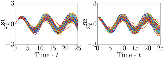
Figure 1. Examples of realizations of x^S for a Fourier Form process with parameters ${\sigma }_w^S=0.01$ and p = 10.

Although the Fourier form component is computationally efficient, it is limited to modeling simple harmonic periodic phenomena such as the one presented in Figure 2A. It is possible to model simple non-harmonic periodic phenomena such as the one presented in Figure 2B using a superposition of Fourier form components each having a different period. Nevertheless this process is in practice difficult, especially when the complexity of the periodic pattern increases because it requires a significant increase in the number of hidden state variables as well as of unknown periods to be identified, which in turn decreases the overall computationally efficiency.

FIGURE 2

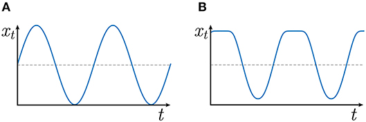
Figure 2. Examples of harmonic (A) and non-harmonic (B) periodic pattern.

2.4.2. Dynamic Regression

In order to overcome the limitations of the Fourier form component, Nguyen and Goulet (2018b) have proposed a new formulation based on the Dynamic Regression component. This approach employs a cubic spline as depicted in Figure 3 for modeling non-harmonic periodic phenomena such as the one presented in Figure 2B. The formulation for this component is

$\begin{array}{ll}{\text{x}}_t^{DR}=x_t^{DR},{\text{A}}_t^{DR}=1,{\text{Q}}_t^{DR}={({\sigma }_w^{DR})}^2,{\text{C}}_t^{DR}=g(t,{\theta }^{DR}).& (8)\end{array}$

FIGURE 3

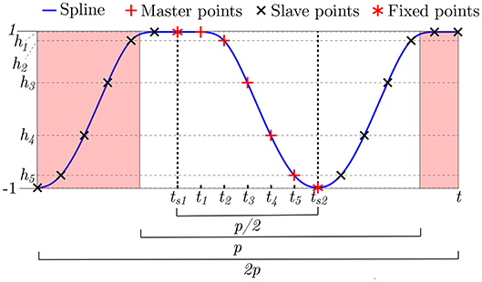
Figure 3. Illustration of the spline employed with the Dynamic regression formulation proposed by Nguyen and Goulet (2018b).

With the dynamic regression component, the hidden state variable $x_t^{DR}$ acts as a regression coefficient that is modulating the amplitude of g(t, θ^DR) which corresponds to the spline presented in Figure 3. The parameters involving this spline are defined as ${\theta }^{DR}={\left[t_{s1},p,\text{h}\right]}^{⊺},\text{h}={\left[h_1,\cdots ,h_N\right]}^{⊺}$, where {θ^DR, h} are learned from data. Although this method has been shown to be capable of modeling complex periodic patterns, its main limitation is that complex periodic patterns typically require a large number (N) of control-point parameters making the approach computationally demanding. The reason behind this computational demand is that control points h need to be estimated with an optimization algorithm (see section 2.3) rather than being treated as hidden state variables that are estimated using the filtering procedure introduced in section 2.2.

2.4.3. Non-parametric Periodic Component

Another alternative to model periodic phenomena is to employ the non-parametric periodic component (West and Harrison, 1999). The mathematical formulation for this component is

$\begin{array}{l}{\text{x}}_t^{NP}={\left[x_{t,1}^{NP},\cdots ,x_{t,N}^{NP}\right]}^{⊺},{\text{A}}_t^{NP}=\left[\begin{array}{cc}0& {\text{I}}_{N-1}\\ 1& 0\end{array}\right],{\text{Q}}_t^{NP}=\left[\begin{array}{cc}{({\sigma }_w^{NP})}^2& 0\\ 0& 0_N\end{array}\right],\\ {\text{C}}_t^{NP}=\left[1,0,\cdots ,0\right],& (9)\end{array}$

where ${\text{x}}_t^{NP}$ is a vector of hidden state variables that are permuted at each time step by the transition matrix ${\text{A}}_t^{NP}$. The advantage of this approach in comparison with the dynamic regression technique is that it can model complex non-harmonic periodic phenomena while having no parameters to be estimated through optimization. This is possible because the signal is modeled using hidden state variables which are estimated recursively. The main limitation of this approach is that it requires as many hidden state variables as there are time steps within the period p of the phenomenon studied. For example, if the phenomenon studied have a period of 1 year and the data's acquisition frequency is Δt = 30 min, it results in 365 × 48 = 17, 520 hidden state variables which is computationally inefficient.

3. Kernel Regression

The new method that employs the concepts of Kernel regression (Henderson and Parmeter, 2015) allows modeling periodic phenomena while overcoming the limitations of the methods presented in section 2.4. This section introduces the theory of Kernel regression on which this paper builds in the following section.

The kernel is employed to measure the similarity between pairs of covariates. The goal here is to model the periodic phenomena in time series, therefore the periodic kernel (Duvenaud, 2014) is formulated as

$\begin{array}{ll}k(t_i,t_j)=exp\left[-\frac{2}{{\ell }^2}sin{\left(\pi \frac{t_i-t_j}{p}\right)}^2\right],& (10)\end{array}$

where the covariate is the time t. The kernel output k(t_i, t_j) ∈ (0, 1) measures the similarity between two timestamps t_i and t_j as a function of the distance between these, as well as a function of two parameters; the period and kernel lengthscale, θ = {p, ℓ}. Figure 4 presents three examples of periodic kernels for different sets of parameters θ. With kernel regression we consider we have a set of observations ${D}=\left\{(t_i,y_i),\forall i=1:D\right\}$ consisting in D pairs of observed system responses y_i, each associated with its time of occurrence t_i. The regression model is built using a set of control points defined using t^KR ∈ ℝ^N, a vector of time covariates associated with a vector of hidden control point values x ∈ ℝ^N. The observed system responses are modeled following

$\begin{array}{ll}{y}_i={\text{x}}^{⊺}\frac{k(t_i,{\text{t}}^{KR})}{{\displaystyle {\sum }_t}k(t,{\text{t}}^{KR})}+v_i,{\displaystyle \underset{\mathrm{\text{Observation errors}}}{{\displaystyle \underbrace{v:V~{N}(v;0,{\sigma }_v^2),}}}}& (11)\end{array}$

where the predictive capacity of the model comes from the product of the hidden control point values x and the normalized kernel values which measure the similarity between the time t_i and those stored for the control points in t^KR. The main challenge here is to estimate x using the set of observation ${D}$. The likelihood describing the conditional probability of ${D}$ given x is

$\begin{array}{ll}f({D}|\text{x})={\displaystyle \prod _{i=1}^D}{N}\left(y_i;{\text{x}}^{⊺}\frac{k(t_i,{\text{t}}^{KR})}{{\displaystyle {\sum }_t}k(t,{\text{t}}^{KR})},{\sigma }_v^2\right).& (12)\end{array}$

FIGURE 4

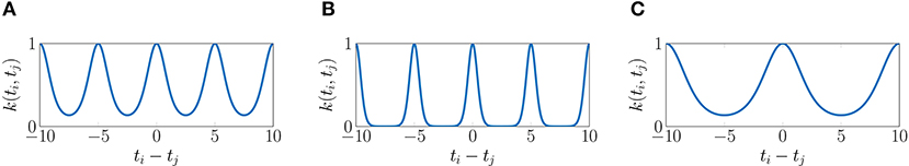
Figure 4. Examples of periodic kernels. (A) θ = {p = 5, ℓ = 1}, (B) θ = {p = 5, ℓ = 0.5}, (C) θ = {p = 10, ℓ = 1}.

If like for the case presented in section 2.3 one employs a MLE approach to estimate x*, the problem consists in maximizing the log-likelihood following

$\begin{array}{ll}{\text{x}}^{*}={\displaystyle \underset{\text{x}}{argmax}}lnf({D}|\text{x}).& (13)\end{array}$

Figure 5 presents an example of application of the Kernel regression in order to model a non-harmonic periodic phenomena. A set of D = 15 simulated observations represented by + symbols are generated by adding normal-distributed observation noise on the ground truth signal presented by the dashed line. Then, an optimization algorithm is employed in order to identify the optimal values x* for a set N = 10 control points represented by the * symbols. This example illustrates the capacity of the kernel-based method on interpolating the system response within control points as well as on extrapolating beyond them.

FIGURE 5

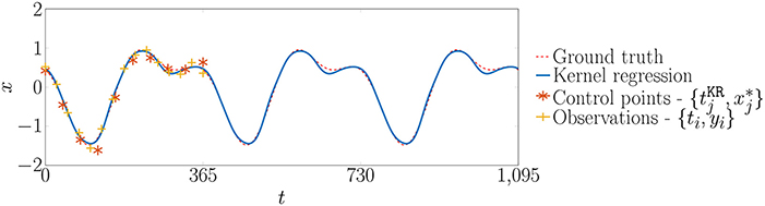
Figure 5. Examples of application of kernel regression.

The main limitation of this approach is that the model cannot involve over time. Moreover, like the Dynamic Regression method presented in section 2.4.2, the estimation of x* relies on a maximization algorithm which makes it computationally inefficient when applied to complex patterns.

4. Using Kernels With BDLM

This section presents the new method proposed in this paper which consists in coupling the Kernel regression method reviewed in section 3 with the Dynamic regression method reviewed in section 2.4.2.

For the new approach, we consider that a vector of N + 1 hidden control point values ${\text{x}}_t^{KR}={\left[x_{t,0}^{KR},x_{t,1}^{KR},\cdots ,x_{t,N}^{KR}\right]}^{⊺}$ is the vector of hidden state variables to be estimated using the filtering procedure presented in section 2.2. Therefore, the transition matrix is defined as

$\begin{array}{ll}{\text{A}}_t^{KR}=\left[\begin{array}{cc}0& {\tilde{k}}^{KR}(t,{\text{t}}^{KR})\\ 0& {\text{I}}_N\end{array}\right],& (14)\end{array}$

where ${\tilde{k}}^{KR}(t,{\text{t}}^{KR})$ corresponds to the normalized kernel, $k(t,{\text{t}}^{KR})/\sum _{t}k(t,{\text{t}}^{KR})$, as presented in Equation (10). ${\tilde{k}}^{KR}(t,{\text{t}}^{KR})$ is parameterized by the kernel lengthscale ℓ^KR, its period p^KR, and a vector of N timestamps ${\text{t}}^{KR}=\left[t_1^{KR},\cdots ,t_N^{KR}\right]$, so that

$\begin{array}{ll}{\tilde{k}}^{KR}(t,{\text{t}}^{KR})\equiv {\tilde{k}}^{KR}(t,{\text{t}}^{KR},{\ell }^{KR},p^{KR})\equiv {\tilde{k}}_t^{KR},& (15)\end{array}$

where each timestamp $t_i^{KR}$ is associated with a hidden control point value $x_{t,i}^{KR}$. The first hidden state variable $x_{t,0}^{KR}$ describes the current predicted pattern value which is obtained by multiplying the remaining N state variables ${\left[x_{t,1}^{KR},\cdots ,x_{t,N}^{KR}\right]}^{⊺}$ and the normalized kernel values contained in the first line of ${\text{A}}_t^{KR}$. From now on, the first and remaining hidden state variables are called the hidden predicted pattern and hidden control points, respectively. The N × N identity matrix forming the bottom right corner of ${\text{A}}_t^{KR}$ indicates that each of the hidden state variables ${\left[x_{t,1}^{KR},\cdots ,x_{t,N}^{KR}\right]}^{⊺}$ evolves over time following a random walk model (West and Harrison, 1999). The temporal evolution of these hidden state variables is controlled by the process noise covariance matrix

$\begin{array}{ll}{\text{Q}}_t^{KR}=\left[\begin{array}{cc}{({\sigma }_0^{KR})}^2& 0\\ 0& {({\sigma }_1^{KR})}^2·{\text{I}}_N\end{array}\right],& (16)\end{array}$

where ${\sigma }_1^{KR}$ controls the increase in the variance of the hidden control points between successive time steps and ${\sigma }_0^{KR}$ controls the time-independent process noise in the hidden predicted pattern. This process noise allows describing random, unpredictable changes in the periodic phenomena between successive time steps. There are four possible cases: (1: ${\sigma }_0^{KR}=0,{\sigma }_1^{KR}=0$) the hidden predicted pattern is stationary and can be exactly modeled by the kernel regression, (2: ${\sigma }_0^{KR}>0,{\sigma }_1^{KR}=0$) the hidden predicted pattern is stationary yet, the kernel regression is an approximation of the true process being modeled (3: ${\sigma }_0^{KR}=0,{\sigma }_1^{KR}>0$) the hidden predicted pattern is non-stationary so the hidden control points values evolve over time and it can be exactly modeled by the kernel regression, (4: ${\sigma }_0^{KR}>0,{\sigma }_1^{KR}>0$) the hidden predicted pattern is non-stationary and it cannot be exactly modeled by the kernel regression. As mentioned, above only the predicted pattern contributes directly to the observation so the observation matrix is

$\begin{array}{ll}{C}_t^{KR}=[1,0,\cdots ,0].& (17)\end{array}$

Because all control points are considered as hidden state variables, the only parameters to be estimated using the MLE procedure presented in section 2.3 are ${\theta }^{KR}={\left[{\sigma }_0^{KR},{\sigma }_1^{KR},{\ell }^{KR},p^{KR}\right]}^{⊺}$.

5. Examples of Application

This section presents two examples of applications using a stationary and a non-stationary case. The first one involves traffic data recorded on a bridge and the second one involves the piezometric pressure recorded under a dam in service.

5.1. Stationary Case—Traffic Load

5.1.1. Data Description

This case-study is conducted on the traffic loading data collected on the Tamar Bridge from September 01 to October 21, 2007 with a total of 2, 409 data points (Goulet and Koo, 2018). Figure 6 presents the entire dataset. The traffic loading data are recorded from a toll booth where the vehicles are counted and classified by weight classes. Note that the data are collected with a uniform time steps of 30 min and is measured by kiloton (kT) unit. A constant baseline and a periodic pattern with a period of 7 days can be observed from the raw data. The traffic loading on weekends is much lighter than those on weekdays. For most of the day, the traffic load presents a high volume between 8 a.m. and 4 p.m., yet it drops out after 20 p.m. at night. In order to examine the predictive performance, the data are divided into a training set (1, 649 data points) and a test set (760 data points). The unknown model parameters are learned using the training set. The predictive performance is then evaluated using the test set. The test set is presented by the shaded region in Figure 6.

FIGURE 6

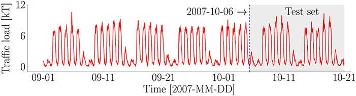
Figure 6. Traffic load on the Tamar Bridge in the United Kingdom.

5.1.2. Model Construction

The model to interpret the traffic load data consists in a vector of hidden states that includes a baseline (B) component to the average of the traffic load, a kernel regression (KR) component with 101 hidden state variables to model the periodic pattern, and an autoregressive (AR) component to captrue the time-dependent model errors. The vector of hidden states is defined as

$\begin{array}{ll}\begin{array}{c}{\text{x}}_t={\left[x_t^B,x_{t,0}^{KR},x_{t,1}^{KR},\cdots ,x_{t,100}^{KR},x_t^{AR}\right]}^{⊺}.\end{array}& (18)\end{array}$

The model involves a vector of unknown model parameters θ that are defined following

$\begin{array}{ll}\theta ={\left[{\sigma }_w^B,{\sigma }_{w,0}^{KR},{\sigma }_{w,1}^{KR},{\ell }^{KR},p^{KR},{\varphi }^{AR},{\sigma }_w^{AR},{\sigma }_v\right]}^{⊺},& (19)\end{array}$

where ${\sigma }_w^B$ is the baseline standard deviation, ${\sigma }_{w,0}^{KR}$ is the standard deviation of the hidden predicted pattern, ${\sigma }_{w,1}^{KR}$ is the standard deviation for the hidden control points, ℓ^KR is the kernel lengthscale, p^KR is the kernel period, ϕ^AR is the autoregression coefficient, σ^AR is the autoregression standard deviation, and σ_v is the observation noise. The standard deviation, kernel lengthscale, and kernel period are positive real number, ℝ⁺. Because the autoregressive component is assumed to be stationary (Rao, 2008), the autoregression coefficient is constrained to the interval (0, 1). For an efficient optimization, the model parameters are transformed in the unbounded space (Gelman et al., 2014). A natural logarithm function is applied to the standard deviation, kernel lengthscale, and kernel period. A sigmoid function is employed for the autoregression coefficient. The complete model matrices are detailed in Appendix A. The initial parameter values in the original space are selected using expert judgment and experience as well as prior data analysis

$\begin{array}{ll}{\theta }^0={\left[10^{-6},0.29,0.029,0.5,7,0.75,0.075,1.47\right]}^{⊺}.& (20)\end{array}$

5.1.3. Parameter and Hidden State Estimation

The optimal model parameters obtained using the MLE technique presented in section 2.3 are

$\begin{array}{ll}{\theta }^{*}={\left[10^{-6},3.3\times 10^{-5},10^{-5},0.0511,7,0.78,0.34,1.2\times 10^{-5}\right]}^{⊺},& (21)\end{array}$

where the ordering of each model parameter remains identical as in Equation 19. Because ${\sigma }_{w,0}^{KR}$ and ${\sigma }_{w,1}^{KR}$, are near to zero, the periodic pattern for this case-study is stationary. Figure 7 presents the hidden state variables and predicted means for the traffic load estimated using Kalman Smoother (Murphy, 2012) for both training set and test set. μ_t|T and σ_t|T are the mean value and standard deviation at time t, respectively, for the hidden state variables. The mean value μ_t|T and its uncertainty bounds μ_t|T ± σ_t|T, are presented by the solid line and shaded region. The estimates for the training set and test set are delimited by the dashed line. The traffic load data is presented by the dash-dot line. The results show that the autoregressive component, $x_t^{AR}$, presented in Figure 7C, is stationary as expected. Because the hidden predicted pattern is stationary, all cycles of 7 days have the identical pattern, as illustrated in Figure 7B. The estimates of the traffic load in the test set are visually close to the corresponding observations, as illustrated in Figure 7D. It can be seen that the model is not capable of predicting the peaks on the test set where the traffic loading presents a high volume in the rush hour. This can be explained by the high variability in the rush hour. The proposed method is intended to captrue the periodic phenomena and not the changes from day to day. The Mean Absolute Error (MAE) and Root Mean Squared Error (RMSE) (Shcherbakov et al., 2013) are employed to measure the forecast accuracy by comparing the estimates with their corresponding traffic-load data in the test set. The mathematical formulation for the MAE and RMSE is presented in Appendix C. These metrics are evaluated on the forecast periods of 1, 3, 7, and 14 days in the test set. The results are summarized in Table 1. The small forecast errors are found for both metrics in each forecast period where the traffic loadings range from 0.07 to 10.3 kT. The forecast error increases with respect to the forecast period.

FIGURE 7

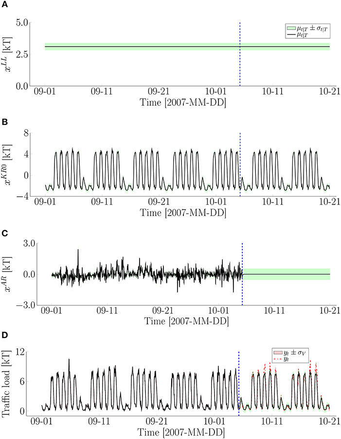
Figure 7. Illustration of the estimation of hidden state variables for the traffic load data: (A) Baseline component, $x_t^B$; (B) Hidden predicted pattern, $x_{t,0}^{KR}$; (C) Autoregressive component, $x_t^{AR}$; (D) Traffic load.

TABLE 1

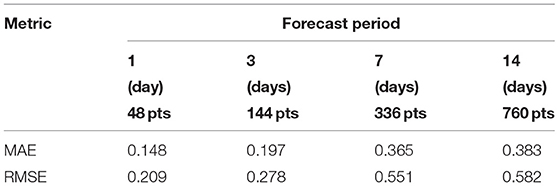
Table 1. Evaluation of forecast accuracy with respect to the different forecast periods for the traffic load data.

5.2. Non-stationary Case—Piezometer Under a Dam

5.2.1. Data Description

For this case-study, the new approach is applied to the piezometric pressure recorded from 2007 to 2016 under a dam in Canada. Note that the piezometric pressure is measured by water meters (wm) unit. The entire dataset with a total of 4181 data points, is presented in Figure 8. The time-step length varies in the range from 1 to 456 h, in which the most frequent time-steps is 12 h. A descending trend and a periodic pattern can be observed from the raw data. Note that the data points for the training set and test set are 2, 538 and 1, 643, respectively. The data is recorded with a non-uniform time-step length, as illustrated in Figure 9.

FIGURE 8

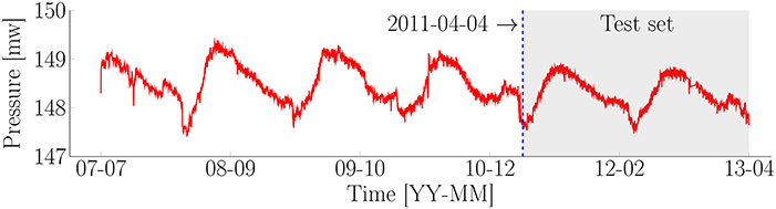
Figure 8. Piezometric pressure under a dam in Canada.

FIGURE 9

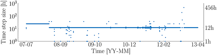
Figure 9. Time-step length for the piezometric pressure data.

5.2.2. Model Construction

The vector of hidden states being used for the model in this case-study includes a baseline (B) component, a local trend (T) component, a kernel regression components (KR), and an autoregressive component (AR). The baseline and local trend components are used for modeling the behavior of piezometric pressure. The kernel regression component associated with 21 hidden state variables, is employed to describe the periodic pattern. The time-dependent errors are modeled by the autoregressive component. The vector of hidden states are written as

$\begin{array}{l}\begin{array}{cc}{\text{x}}_t={\left[x_t^B,x_t^T,x_{t,0}^{KR},x_{t,1}^{KR},\cdots ,x_{t,20}^{KR},x_t^{AR}\right]}^{⊺}.& (22)\end{array}\end{array}$

The unknown model parameters relating to these hidden states are defined as

$\begin{array}{ll}\theta ={\left[{\sigma }_w^T,{\sigma }_{w,0}^{KR},{\sigma }_{w,1}^{KR},{\ell }^{KR},p^{KR},{\varphi }^{AR},{\sigma }_w^{AR},{\sigma }_v\right]}^{⊺},& (23)\end{array}$

where ${\sigma }_w^T$ is the local-trend standard deviation and the remaining model parameters have the same with the bounds presented in Equation (19). These model parameters are also transformed in the unconstrained space for the optimization task. The full model matrices are presented in Appendix B. The initial parameter values in the original space are regrouped following

$\begin{array}{ll}{\theta }^0={\left[10^{-6},0.37,0.018,0.5,365.24,0.75,0.075,0.018\right]}^{⊺}.& (24)\end{array}$

5.2.3. Parameter and Hidden State Estimation

The vector of optimal model parameters are obtained following

$\begin{array}{ll}{\theta }^{*}={\left[3.6\times 10^{-6},0.047,0.015,0.485,363.07,0.91,0.035,4.5\times 10^{-5}\right]}^{⊺},& (25)\end{array}$

where the ordering of each model parameters is the same as in Equation 23. Because ${\sigma }_{w,0}^{KR}$ and ${\sigma }_{w,1}^{KR}$ are different from zero, the hidden predicted pattern is non-stationary. The hidden state variables and estimates for the piezometric pressure are shown in Figure 10. The mean values μ_t|T and its uncertainty bounds μ_t|T ± σ_t|T are presented by the solid line and shaded region, respectively. The dashed line is used to separate the estimates between the training set and test set. The dash-dot line presents the piezometric pressure data. According to the results, the autoregressive component, $x_t^{AR}$, presents a stationary behavior in the training set, as shown in Figure 10C. The non-stationarity in the hidden predicted pattern can be observed in Figure 10B where each cycle of 363 days is different from each other. Figure 10D shows that the distance between the estimates for the first year in the test set and their corresponding observation is further than the one for the second year. Yet, the uncertainty bounds for the first year remain smaller than those for the second year. In addition, the uncertainty bounds of the estimates in the test set include most of the corresponding pressure data. The MAE and RMSE are also employed for measuring the forecast accuracy for such as this case-study. Table 2 shows the forecast error of two metrics with respect to the forecast periods of 30, 180, 365, and 730 days. The forecast errors are small for each forecast period in which the piezometric pressure data varies in range from 147.5 to 148.9 water meters. The forecast error is large as the forecast period grows from 30 to 365 days. However, it is slightly reduced for the forecast period of 730 days. This can be explained by the better estimates for the second year in the test set.

FIGURE 10

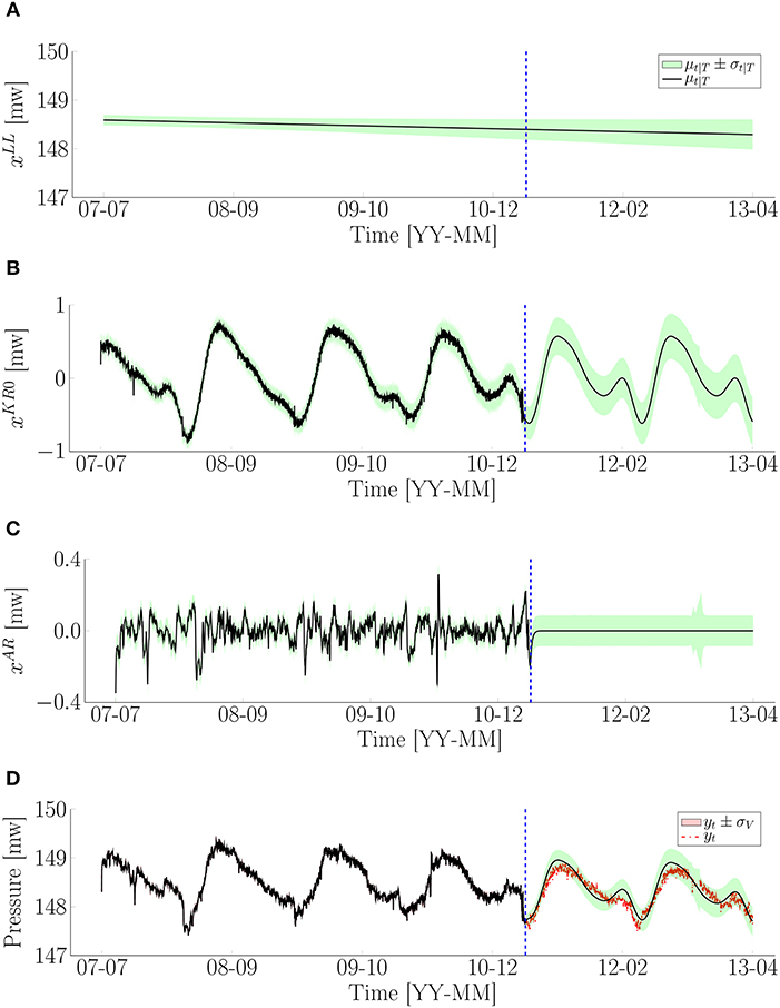
Figure 10. Illustration of the estimation of hidden state variables for the piezometric pressure data: (A) Baseline component, $x_t^B$; (B) Hidden predicted pattern, $x_{t,0}^{KR}$; (C) Autoregressive component, $x_t^{AR}$; (D) Pressure.

TABLE 2

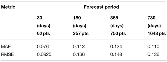
Table 2. Evaluation of forecast accuracy for the different forecast periods on the piezometric pressure data.

6. Discussion

The analysis of the traffic load and pressure time-series data shows that coupling the periodic kernel regression with BDLM enables to model non-harmonic periodic patterns recorded in different settings. The results from the traffic-load data allow investigating the performance of the approach to model a stationary periodic pattern observed regularly over time, but that exhibits a complex shape. The results from the pressure data allow interpreting the performance of the approach on a simple non-stationary periodic pattern observed irregularly over time.

In contrast with the dynamic regression technique presented in section 2.4.2, the proposed approach takes advantage of the Kalman computations to estimate analytically and recursively the periodic pattern. Therefore, the approach is computationally efficient. The use of Kalman computations also naturally provide uncertainty bound around the prediction, which is crucial for time series forecasting. The use of a kernel in the proposed approach enables to process observations collected at irregular time interval, which is not possible with the non-parametric periodic component, as presented in section 2.4.3. In addition, it can handle non-stationary periodic patterns. The non-stationarity is accommodated by imposing a random walk on each hidden control points, which is mainly controlled by the standard deviation ${\sigma }_{w,1}^{KR}$. In common cases, the time series cannot be visually inspected before analysis, and therefore, the model parameter ${\sigma }_{w,1}^{KR}$ is learned from the data using the MLE procedure. Starting from ${\sigma }_{w,1}^{KR}$ values of 0.029 and 0.18 for the traffic load and pressure data, respectively, the MLE procedure is capable to converge to ${\sigma }_{w,1}^{KR}$ values of 10⁻⁵ and 0.015, respectively, thus highlighting the non-stationarity of the periodic pattern in the pressure data compared to the one observed in the traffic load data. The process noise standard deviation ${\sigma }_{w,0}^{KR}$ associated with the hidden periodic pattern is also learned from the data. Initializing at ${\sigma }_{w,0}^{KR}$ values of 0.29 and 0.37 for the traffic load and pressure data, respectively, the MLE procedure is capable to converge to ${\sigma }_{w,0}^{KR}$ values of 3.3 × 10⁻⁵ and 0.047, respectively. The high values for ${\sigma }_{w,0}^{KR}$ and ${\sigma }_{w,1}^{KR}$ obtained from the pressure training dataset explain the shift in both amplitude and phase found in the estimates of the pressure test dataset, as illustrated in Figure 10D.

The kernel period, p^KR, is another crucial model parameter. Unlike the model parameters ${\sigma }_{w,0}^{KR}$ and ${\sigma }_{w,1}^{KR}$ discussed above, a good initial guess of the period should be provided for ensuring an efficient optimization. The reason is that the likelihood of the observation given the period is strongly peaked, and starting at the wrong value can lead to a slow convergence. Moreover, the likelihood about the period may also have several maxima if the time series contains several periods, which may lead the MLE procedure to converge toward a local maximum. The use of a periodogram for identifying the dominant period may be misleading, because the dominant period may not be the period that is the most suited for the kernel period. For example, the dominant period in the traffic loading example is 1 day, yet it can be observed that there is a difference in amplitude between the weekdays and weekends. Therefore, a period of 1 day might yield poor predictive results for such as case. For practical applications, the visualization of the time-series is the best way for identifying good starting values for the period prior analysis. In addition, multiple sets of initial parameter values should be tested during the optimization procedure.

Furthermore, the number of hidden control points is a hyperparameter to be tuned before the analysis. This hyperparameter can be identified using the cross-validation technique (Bergmeir and Benítez, 2012). The cross-validation consists in splitting the data into the training set and validation set in which the model is trained on the training set. The hyperparameter that minimizes the error on the validation set is selected. Moreover, it is important to note that the kernel function allows interpolating between hidden control points, thus enabling simple models (i.e., with few control points) to fit a large diversity of periodic patterns.

7. Conclusion

This study proposes a novel approach for modeling the non-harmonic periodic patterns in time-series for the context of Structural Health Monitoring. The technique combines the formulation of the existing Bayesian dynamic linear models with a kernel-based method. The application of the method on two case studies illustrates its potential for interpreting complex periodic time series. The results show that the proposed approach succeeds in modeling the stationary and non-stationary periodic patterns for both case studies. Also, it is computationally efficient, versatile, self-adaptive to changing conditions, and capable of handling observations collected at irregular time intervals.

Author Contributions

LHN, IG, SK, and J-AG wrote the paper together and conceived the case-study examples. J-AG and LHN formulated the mathematical formulation for the proposed method. LHN and SK performed the simulation.

Funding

This project is funded by the Natural Sciences and Engineering Research Council of Canada (NSERC), Hydro Québec (HQ), Hydro Québec's Research Institute (IREQ), and Institute For Data Valorization (IVADO).

Conflict of Interest Statement

The authors declare that the research was conducted in the absence of any commercial or financial relationships that could be construed as a potential conflict of interest.

References

Álvarez, M. A., Rosasco, L., and Lawrence, N. D. (2012). Kernels for vector-valued functions: a review. Found. Trends Mach. Learn. 4, 195–266. doi: 10.1561/2200000036

CrossRef Full Text | Google Scholar

Bergmeir, C., and Benítez, J. M. (2012). On the use of cross-validation for time series predictor evaluation. Information Sci. 191, 192–213. doi: 10.1016/j.ins.2011.12.028

CrossRef Full Text | Google Scholar

Bishop, C. (2006). Pattern Recognition and Machine Learning. Singapore: Springer.

Google Scholar

Duvenaud, D. (2014). Automatic Model Construction With Gaussian Processes. Ph.D. thesis, University of Cambridge.

Google Scholar

Gamse, S., and Oberguggenberger, M. (2017). Assessment of long-term coordinate time series using hydrostatic-season-time model for rock-fill embankment dam. Struct. Control Health Monitor. 24:e1859. doi: 10.1002/stc.1859

CrossRef Full Text | Google Scholar

Gelman, A., Carlin, J. B., Stern, H. S., and Rubin, D. B. (2014). Bayesian Data Analysis, 3 Edn. New York, NY: CRC Press.

Google Scholar

Goulet, J.-A. (2017). Bayesian dynamic linear models for structural health monitoring. Struct. Control Health Monitor. 24, 1545–2263. doi: 10.1002/stc.2035

CrossRef Full Text | Google Scholar

Goulet, J.-A., and Koo, K. (2018). Empirical validation of Bayesian dynamic linear models in the context of structural health monitoring. J. Bridge Eng. 23:05017017. doi: 10.1061/(ASCE)BE.1943-5592.0001190

CrossRef Full Text | Google Scholar

Henderson, D. J., and Parmeter, C. F. (2015). Applied Nonparametric Econometrics. Cambridge University Press.

Google Scholar

Léger, P., and Leclerc, M. (2007). Hydrostatic, temperatrue, time-displacement model for concrete dams. J. Eng. Mech. 133, 267–277. doi: 10.1061/(ASCE)0733-9399(2007)133:3(267)

CrossRef Full Text | Google Scholar

Mata, J. (2011). Interpretation of concrete dam behaviour with artificial neural network and multiple linear regression models. Eng. Struct. 33, 903–910. doi: 10.1016/j.engstruct.2010.12.011

CrossRef Full Text | Google Scholar

Michalak, M. (2011). “Time series prediction with periodic kernels,” in Computer Recognition Systems 4, eds R. Burduk, M. Kurzyński, M. Woźniak, and A. Żołnierek (Berlin; Heidelberg: Springer Berlin Heidelberg), 137–146.

Google Scholar

Murphy, K. (2012). Machine Learning: A Probabilistic Perspective. London, UK: The MIT Press.

Google Scholar

Nguyen, L., and Goulet, J.-A. (2018a). Anomaly detection with the switching kalman filter for structural health monitoring. Struct. Control Health Monitor. 25:e2136. doi: 10.1002/stc.2136

CrossRef Full Text | Google Scholar

Nguyen, L., and Goulet, J.-A. (2018b). Structural health monitoring with dependence on non-harmonic periodic hidden covariates. Eng. Struct. 166, 187–194. doi: 10.1016/j.engstruct.2018.03.080

CrossRef Full Text | Google Scholar

Prado, R., and West, M. (2010). Time Series: Modeling, Computation, and Inference, 1st Edn. New York, NY: Chapman & Hall/CRC.

Google Scholar

Rao, S. S. (2008). A Course in Time Series Analysis. Technical report, Texas A&M University.

Google Scholar

Salazar, F., and Toledo, M. (2018). Discussion on “thermal displacements of concrete dams: accounting for water temperatrue in statistical models”. Eng. Struct. 171, 1071–1072. doi: 10.1016/j.engstruct.2015.08.001

CrossRef Full Text | Google Scholar

Särkkä, S. (2013). Bayesian Filtering and Smoothing, Vol. 3. New York, NY: Cambridge University Press.

Google Scholar

Scholkopf, B., and Smola, A. J. (2001). Learning with Kernels: Support Vector Machines, Regularization, Optimization, and Beyond. Cambridge, MA: MIT Press.

Google Scholar

Shcherbakov, M. V., Brebels, A., Shcherbakova, N. L., Tyukov, A. P., Janovsky, T. A., and Kamaev, V. A. (2013). A survey of forecast error measures. World Appl. Sci. J. 24, 171–176. doi: 10.5829/idosi.wasj.2013.24.itmies.80032

CrossRef Full Text | Google Scholar

Simon, D. (2006). Optimal State Estimation: Kalman, H Infinity, and Nonlinear Approaches. New Jersey, NJ: Wiley.

Google Scholar

Solhjell, I. (2009). Bayesian Forecasting and Dynamic Models Applied to Strain Data from the Göta river Bridge. Master's thesis, University of Oslo.

Google Scholar

Tatin, M., Briffaut, M., Dufour, F., Simon, A., and Fabre, J.-P. (2015). Thermal displacements of concrete dams: accounting for water temperatrue in statistical models. Eng. Struct. 91, 26–39. doi: 10.1016/j.engstruct.2015.01.047

CrossRef Full Text | Google Scholar

West, M., and Harrison, J. (1999). Bayesian Forecasting and Dynamic Models. New York, NY: Springer.

Google Scholar

Westgate, R., Koo, K.-Y., and Brownjohn, J. (2015). Effect of vehicular loading on suspension bridge dynamic properties. Struct. Infrastruct. Eng. 11, 129–144. doi: 10.1080/15732479.2013.850731

CrossRef Full Text | Google Scholar

Appendix A

The model matrices {A_t, C_t, Q_t, R_t} for the case-study of traffic load data are defined following

$A_t=\text{block}\text{diag }\left(\text{1},\left[\begin{array}{cc}\text{0}& {\tilde{\text{k}}}_{\text{t}}^{\text{KR}}\\ 0& I_{\text{100}}\end{array}\right],{\varphi }^{\text{AR}}\right)$

$C_t=[1,1,0_1,0_2,\cdots ,0_{100},1]$

$R_t=\left[{\left({\sigma }_v\right)}^2\right]$

$Q_t=\text{block}\text{diag }\left({\left({\sigma }_{\text{w}}^{\text{B}}\right)}^{\text{2}},\left[\begin{array}{cc}{\left({\sigma }_{\text{w},\text{0}}^{\text{KR}}\right)}^{\text{2}}& 0\\ 0& {\left({\sigma }_{\text{w},\text{1}}^{\text{KR}}\right)}^{\text{2}}·I_{\text{100}}\end{array}\right],{\left({\sigma }_{\text{w}}^{\text{AR}}\right)}^{\text{2}}\right),$

where ${\tilde{k}}_t^{KR}=\left[{\tilde{k}}_{t,1}^{KR},{\tilde{k}}_{t,2}^{KR},\cdots ,{\tilde{k}}_{t,100}^{KR}\right]$ is the normalized kernel values.

Appendix B

The model matrices {A_t, C_t, Q_t, R_t} for the case-study of piezometric pressure data are defined following

$A_t=\text{block}\text{diag }\left(\left[\begin{array}{cc}\text{1}& \Delta \text{t}\\ \text{0}& \text{1}\end{array}\right],\left[\begin{array}{cc}\text{0}& {\tilde{k}}_{\text{t}}^{\text{KR}}\\ 0& I_{\text{20}}\end{array}\right],{\varphi }^{\text{AR}}\right)$

$C_t=[1,0,1,0_1,0_2,\cdots ,0_{20},1]$

$R_t=\left[{\left({\sigma }_v\right)}^2\right]$

$Q_t=\text{block}\text{diag }\left({\left({\sigma }_{\text{w}}^{\text{B}}\right)}^{\text{2}}·\left[\begin{array}{cc}\frac{\Delta {\text{t}}^{\text{3}}}{\text{3}}& \frac{\Delta {\text{t}}^{\text{2}}}{\text{2}}\\ \frac{\Delta {\text{t}}^{\text{2}}}{\text{2}}& \Delta \text{t}\end{array}\right],\left[\begin{array}{cc}{\left({\sigma }_{\text{w},\text{0}}^{\text{KR}}\right)}^{\text{2}}& 0\\ 0& {\left({\sigma }_{\text{w},\text{1}}^{\text{KR}}\right)}^{\text{2}}·I_{\text{20}}\end{array}\right],{\left({\sigma }_{\text{w}}^{\text{AR}}\right)}^{\text{2}}\right)$

where ${\tilde{k}}_t^{KR}=\left[{\tilde{k}}_{t,1}^{KR},{\tilde{k}}_{t,2}^{KR},\cdots ,{\tilde{k}}_{t,20}^{KR}\right]$ is the normalized kernel values and Δt is the time step at the time t.

Appendix C

The mathematical formulations for the Mean Absolute Error (MAE) and Root Mean Squared Error (RMSE) are written as following

$\begin{array}{l}\begin{array}{c}\mathrm{\text{MAE}}=\frac{1}{T}{\displaystyle \sum _{t=1}^T}|\widehat{y_t}-y_t|\\ \mathrm{\text{RMSE}}=\sqrt{\frac{{\displaystyle \sum _{t=1}^T}{(\widehat{y_t}-y_t)}^2}{T}},\end{array}\end{array}$

where ŷ_t is the forecast value and y_t is the observation at time t.