Stochastic Track Model for Tornado Risk Assessment in the U.S.

Introduction

On average, the continental United States is subjected to more than 1,000 tornadoes every year, causing significant financial losses and social disruption. The Storm Prediction Center (SPC), a division of the National Oceanic and Atmospheric Administration (NOAA), maintains a database of tornado events recorded since 1950. The annually observed number of tornadoes, or annual occurrence rate, appears to be increasing (Figure 1). This could be due in part to the improvement of technology used for tracking tornadoes, such as Doppler radar, and public awareness in reporting tornado incidents. Compared to a hurricane, the influence area of a tornado is relatively small. Even with over 60,000 of known historical tornado events in the SPC database, many places in tornado prone region have not been hit by a tornado. Therefore, it is not feasible to directly determine the risk due to tornadoes for a location or small region using solely the observed tornado events.

FIGURE 1

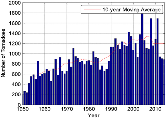
Figure 1. Annual number of tornadoes recorded from 1950 to 2015 and 10 year moving average.

Quantifications of tornado hazard and its impact on the built environment are subjects of study by many over the years. Prior tornado climatology research has relied mainly on the spatial and temporal variation of tornado spawn days over a fixed period to quantify tornado risk (e.g., Brooks et al., 2003; Farney and Dixon, 2014). Standohar-Alfano and van de Lindt (2015) divided the continental US into various grid sizes and simulated the annual tornado occurrence probability using the minimum assumption method proposed by Schaefer et al. (1986) in which the tornado occurrence probability is estimated using the sum of the tornado areas divided by the total observation years and the area of the grid of interest. Sigal et al. (2000) simulated multiple realizations of 100,000 years of tornado events for the continental of the US using Latin hypercude method. The simulated results were then used to estimate average annual loss (AAL) for different regions. They concluded that 100,000 years of simulation are not adequate to obtain convergence for AAL. This is likely attributed to very small influence area of tornado.

Boruff et al. (2003) found that while the number of reported tornado events were almost doubled from 1950 to 2000, there has been a steady reduction in tornado induced fatalities and injuries in recent years. This is likely attributed to the advancement made in forecasts and warning times of tornado outbreaks. While the overall fatality rate has reduced, the analyses by Ashley (2007) and Ashley et al. (2008) confirmed the common perception that nocturnal tornadoes caused higher fatalities than tornadoes spawned during the daytime.

Thom (1963) analyzed the distributions of tornado path width and length using tornado data for Iowa and Kansas. He found that more than 90% of the Iowa tornadoes had easterly paths. A more recent study by Suckling and Ashley (2006) examined more than 6,000 tornado tracks from 1980 to 2002. They found that while tornadoes generally travel in paths from the southwest toward the northeast direction, in central and northern region of the US, a more westerly tornado paths preponderates during late spring and summer. These studies showed that the spatial and temporal characteristics of tornado paths should be considered. Tan and Hong (2010) developed tornado hazard maps for Southern Ontario in Canada and they also showed that the spatial inhomogeneity of tornado occurrence is an important factor that must be considered when developing tornado hazard maps. In order to simulate the temporal and spatial dependent of tornado tracks, a stochastic simulation program for generating synthetic tornado tracks based on the statistics of historical data was developed in this paper.

The Monte Carlo Simulation (MCS) technique was employed in this study to develop the tornado simulation program. MCS is a computational method that utilizes repeated sampling of random numbers from a sequence of probability distributions to obtain the behaviors or responses of a relatively complex system or phenomena with random outcomes. The MCS technique has been widely used to assess the risk of natural hazards with relatively rare occurrences. Meyer et al. (2002) employed the MCS approach to study significant tornado occurrence distribution in the continental of the United States. Strader et al. (2016) developed a MCS model for simulating tornado events applied to a user-defined domain to estimate tornado impacts on the built environment. Daneshvaran and Morden (2007) evaluated the spatial frequency of occurrence of tornadoes in the United States and estimated the losses of tornado and hail outbreaks. Banik et al. (2008) used a stochastic model for assessing the exceedance probability of maximum tornado wind speed in Southern Ontario, Canada.

One of the key contributions of the tornado simulation methodology developed in this study is the use of kernel density estimation (KDE) and MCS methods to generate geographic dependent tornado parameters, which include the EF-scale, path length, maximum path width, path direction, spawn month, date, and hours. Many previous studies did not consider the tornado spawn month or time (Daneshvaran and Morden, 2007; Banik et al., 2012; Standohar-Alfano and van de Lindt, 2016), even though the spawn timing of tornadoes has been shown to play an important role in risk assessment. According to the study by Simmons and Sutter (2010), the fatalities were 15% higher for tornadoes occurred during offseason compared to tornado season from March to June. In addition, it has been shown that nocturnal tornadoes have higher fatality rate than diurnal tornadoes (Ashley, 2007; Ashley et al., 2008). While advancement in technology and early warning system has greatly reduced the overall number of casualties due to tornadoes, the fatality rates for nocturnal tornadoes remained largely unchanged over the years. Ashley et al. (2008) found that nocturnal tornadoes occurring during midnight to sunrise of local time are 2.5 times more likely to kill that those tornadoes occurring during the day time. Therefore, it is very important to have a model that can explicitly simulate geographic dependent tornado parameters such as EF-scale, path length, path width, spawn month, and spawn time in a day, in particular, when the model is intended for use in estimating occupant risk or casualty.

Method of Analysis

Analysis Procedure

The main procedure used to simulate the geographic dependent tornado tracks is present in Figure 2, and discussed in this paper according to the following organization:

FIGURE 2

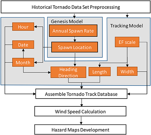
Figure 2. Flowchart of tornado track simulation procedures.

1) Data pre-processing (section Data Sources): the historical tornado database was pre-processed to remove incomplete data set and reconcile inconsistent entries.

2) Stochastic model development (section Genesis model to Wind field model): the stochastic tornado simulation model contains three sub-models, (i) genesis model which is used to determine the spawn frequency and location; (ii) tracking model which is used to simulate the track parameter such as path width, length, heading direction and intensity; (iii) windfield model which is used to compute the wind speeds within the tornado footprint.

3) Tornado track simulation: using the developed stochastic tornado simulation program, a tornado database which contains 1 million years of simulated tornado tracks was generated using a high performance computing cluster.

4) Model validation and hazard maps development (section Synthetic tornado tracks database and applications): the statistics of the simulated tornado tracks are compared to historical observations to verify that the simulated tornado hazard matches the observed trend. Using the computed peak wind speeds, a series of tornado hazard maps are developed and a potential application of the simulated tornado database is also presented.

Data Sources

There are two tornado databases that are widely used in tornado related research: (1) the Grazulis database contains over 10,000 tornadoes for the period of 1921–1995; (2) the NOAA database with over 60,000 tornadoes for the period of 1950 to present. Both of these databases contain detailed tornado track information such as, spawn location (latitude and longitude), starting time, width, length, and damage classification. However, the Grazulis database only includes F2 and higher intensity tornadoes prior to 1995. It should be noted that the well-known Fujita scale tornado intensity classification system was proposed by Dr. Theodore Fujita in 1971 and it was not incorporated into the tornado rating until 1973. The enhanced Fujita (EF) scale was later introduced in 2007. Instead of determining the tornado intensity based on field measurement using the “degree of damage” scale, recorded tornado intensities before 1973 were assigned purely according to the newspaper reports or photographs of the affected regions. Note that both F scale and EF scale are damage based rating system and the numerical categories of both scales are intended to be consistent in terms of the impact or damage to structures. Based on much work from post-tornado field investigations and observations from Doppler radar, the wind speeds associated with the original Fujita scale were deemed too high. This led to the development of the EF scale and the re-assignment of the wind speeds. Since the data set from SPC contains both F and EF scales, a direct mapping of F scale ratings into EF scale is used in this study (e.g., F0 is treated the same as EF0).

Figure 1 shows the tornado annual spawn frequency for the continental of the US and the 10-year moving average from 1950 to 2015. The annual spawn frequency in the 1990s increased by 60% com-pared to the 1950s and increased by 30% compared to 1970s. The observed increased spawn rate in recent decades is likely due to the implementation of Doppler radar network in the early 1990s. In other words, the annual spawn frequency records prior to 1990 may be underestimated.

Stochastic Track Simulation Model

The main simulation model includes two sub-models, namely, the genesis model and track model. The genesis model is used to simulate the tornado annual occurrence rate and spawn locations. The track model is utilized to simulate the tornado track parameters (such as intensity, heading direction, width etc.) according to its spawn location. The parameters of each simulated tornado include the intensity (EF scale), touchdown location in terms of the latitude and longitude, touchdown date and time, path length, path width and heading direction.

The parameters of the simulated tornadoes in this study are geographic dependent. In other words, the tornado parameters (e.g., EF scale) are sampled from probability distributions that vary based on geographic location. For example, the likelihood of a major tornado (EF 4 or EF 5) spawns in Kansas, a tornado prone area, is expected to be significantly higher than that in a location along the eastern coast of the United States. To achieve a geographic dependent simulation, the Kernel Density Estimation method (KDE) is applied in both the genesis model and the track model. The KDE method is one of the most commonly used spatial analytical techniques, which is often used to quantify the spatial variation of the probability density of a random variable. A bivariate normal distribution is utilized to as the kernel density estimator. The probability density function (PDF) of the bivariate normal distribution is:

$\begin{array}{cc}f\left(x,y\right)=\frac{1}{2\pi {\sigma }_X{\sigma }_Y\sqrt{1-{\rho }^2}}exp\left(-\frac{1}{2\left(1-{\rho }^2\right)}\left[\frac{{\left(x-{\mu }_X\right)}^2}{{\sigma }_X^2}+\frac{{\left(y-{\mu }_Y\right)}^2}{{\sigma }_Y^2}-\frac{2\rho (x-{\mu }_X)(y-{\mu }_Y)}{{\sigma }_X{\sigma }_Y}\right]\right)& (1)\end{array}$

Where, μ_x and μ_y are the longitude and latitude of the observed spawn location of each tornado. σ_x and σ_y are the bandwidths for longitudinal and latitudinal directions, respectively, and ρ is the correlation coefficient. The bandwidths represent the likely deviations or drifts of spawn locations of future tornadoes from the known observed locations. In this study, it is assumed that the future spawn locations of tornadoes are equally likely to drift away from the past observed locations in the longitudinal and latitudinal directions, and there is no correlation between the two directions. In other words, σ_x is equal to σ_y and ρ is taken as zero. As a result, there is only one free parameter to be estimated in Equation 1, which is the bandwidth, σ (i.e., σ_x = σ_y = σ).

The problem at hand is to select an optimal bandwidth for each tornado parameter. An overly large bandwidth may result in over-smoothed estimation, suppressing the actual underlying structure of the probability density distribution. In contrast, if a small bandwidth is applied, the estimated density function may contain spurious statistical artifacts and sharp changes in probability density values between close proximity locations. The bandwidth selection technique via diffusion proposed by Botev et al. (2010) is applied to determine the bandwidth in this study. The selection via diffusion algorithm evaluates the best-fit bandwidth according to the spatial distribution and size of the sample space. Compared to the commonly used mean integrated squared error method, the bandwidth selection via diffusion approach is computational efficiency and it better suited for estimating multimodal density function.

Genesis Model

According to the previous research by Standohar-Alfano and van de Lindt (2015), negative binominal distribution was determined to be a distribution suitable for describing the tornado annual frequency. The PDF of the negative binomial distribution is given by:

$\begin{array}{cc}Pr\left(X=N_{Tor}\right)=\left(\stackrel{N_{Tor}+r-1}{N_{Tor}}\right)p^{N_{Tor}}{(1-p)}^r& (2)\end{array}$

where N_Tor is the number of tornados occurred in a year. p = 0.0253 and r = 31.605 are the distribution parameters fitted using the observed annual spawn rates of the SPC database. The p and r parameters were estimated via the maximum likelihood method using the SPC data from 1990 to 2015. As previously discussed, the spawn rates prior to 1990 are excluded because it is believed that the dataset may be underestimated due to poor observation coverage.

The quantile-quantile (Q-Q) plot is utilized to judge the quality of fit of the observed and modeled probability distributions by plotting their quantiles against each other. If the observed and modeled probabilities have identical distributions, the points in Q-Q plot will approximately lie on a straight diagonal (45-degree) line. In Figure 3, the modeled tornado annual occurrence rates are plotted on the x-axis, and the corresponding quantile values from the actual observations are plotted on the y-axis. The red dots in Figure 3 represent the 10th, 20th, 30th to 90th percentiles of the two probability distributions. According to the observation, most of the points are close to the 45-degree line which means the fitted negative binomial distribution can be used to model the annual spawn rate of tornadoes in the US. It should be noted that the fitted probability distribution model deviates slightly from the empirical dataset in region of high annual occurrence rates (>1,500 tornadoes/year) or beyond the 90th percentile.

FIGURE 3

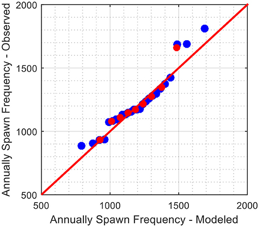
Figure 3. Quantile-to-quantile plot of observed versus modeled annual tornado spawn frequencies.

To consider the variation in tornado occurrences due to climatological differences in the US (Kelly et al., 1978; Farney and Dixon, 2014), this study modeled the tornado touchdown location as a geographic dependent parameter. Each simulated tornado spawn location is randomly generated using a bivariate normal random number generator with an optimal bandwidth (Equation 1). The random number generator returns a random location chosen from the bivariate normal distribution with input means (μ_x and μ_y), and variance (σ), where the means control the center location of the distribution and σ controls the dispersion of the distribution (bandwidth). The means (latitude and longitude) are sampled from the known spawn locations of historical events and variance (σ) is obtained from the previously discussed KDE by diffusion method.

The tornado genesis model simulation procedures are as follows:

1) Randomly sample a tornado annual spawn rate (N_Tor) from the negative binominal distribution (p = 0.0253, r = 31.605);

2) Randomly select a tornado year (1950–2015) and use all the observed tornadoes in that particular year to generate the KDE of the spawn locations with an optimal bandwidth;

3) Randomly select N_Tor spawn locations with replacement using all the observed tornadoes of the selected year in step 2;

4) Use the KDE method to vary the spawn locations determined in step 3 (i.e., use a bivariate normal distribution with the center (μ_x and μ_y) equal to the initial spawn locations determined in step 3 and the variance (σ) equal to the optimal KDE bandwidth determined in step 2 to randomize the final spawn locations).

During the genesis process, if the randomized spawn location of a tornado is outside of the US land boundary (i.e., in ocean), step 4 is repeated until that particular tornado is inside the US land boundary. To preserve the local climatological patterns, instead of aggregating all historical spawn locations to generate one KDE map, a KDE model for spawn location is produced for each simulation year. Figure 4 shows an example simulation year with spawn locations of tornadoes derived based on the tornadoes of year 1992 as the seeds. The probability density contours of both the modeled and observed tornado spawn locations are shown in Figures 4A,B, respectively. As can be seen, the modeled tornadoes follow the spatial pattern of the observed tornado distribution very well. Both the observed and modeled tornado spawn KDE contours show high probabilities of occurrence in the northwest region of Kansas and near Louisiana.

FIGURE 4

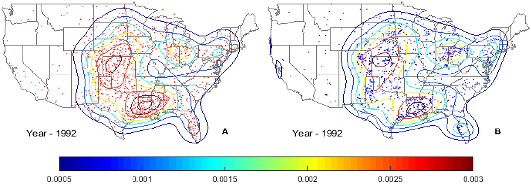
Figure 4. Probability density contours of tornado spawn locations for (A) modeled, and (B) observed tornadoes using the tornadoes spawned in year 1992 as the seeds.

Track Model

For each tornado spawned using the genesis model, six additional tornado parameters, namely (1) EF-scale (B), (2) path direction (θ, measured clockwise from the true North), (3) spawn month (M), (4) spawn time (H), (5) path length (L), and (6) width (W), are simulated using the track model. To ensure the simulated tornado parameters follow the geographic patterns of historical tornado records, the data for each tornado parameter is divided into subgroups and each subgroup is analyzed separately using the same KDE approach employed for the spawn location model. Table 1 shows the grouping of the four tornado parameters.

TABLE 1

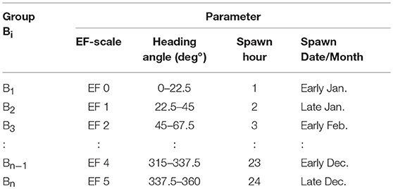
Table 1. Tornado parameter groups.

For a specific tornado parameter, for instance the EF-scale, the historical tornadoes are categorized into different groups (B_i) and each group contains tornadoes with the same characteristic (e.g., EF-scale equal to 2). The tornado spawn records from these grouped datasets are used to generate the probability density contour maps using the KDE method. The KDE contours reflect the spatial distribution and concentration of tornadoes with the same characteristic. The developed probability density contour maps are used to determine the point estimate for probability density of tornadoes at a given location with the specified group of parameter of interest. Figure 5 shows two examples probability density models (maps) developed using only the EF-2 tornadoes (Figure 5A) and only those tornadoes spawned during early January (Figure 5B).

FIGURE 5

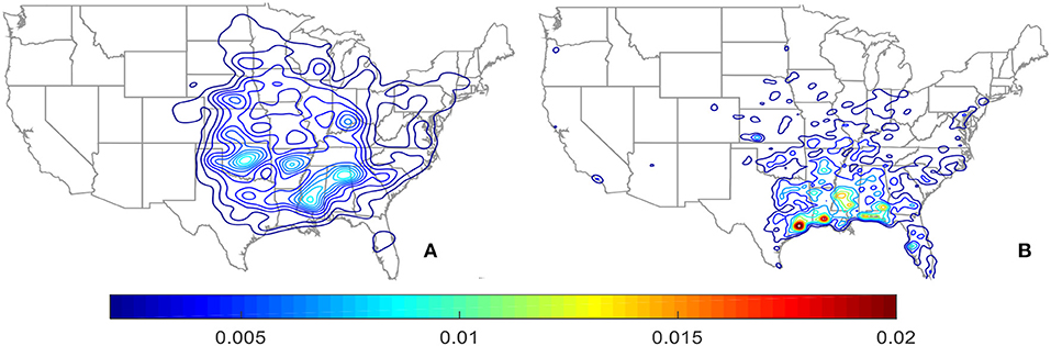
Figure 5. Probability density contours for (A) EF-2 tornadoes and (B) tornadoes spawned in early January.

Once the spawn location of a tornado has been determined using the genesis model, the conditional probability are used to simulate the six tornado parameters. For illustration purpose, consider the determination of EF-scale for a tornado j at location (Lat, Lon)_j. According to the conditional probability, the probability of a tornado occurs at location (Lat, Lon)_j and its EF-scale is equal to B_i is:

$\begin{array}{cc}P\left({(Lat,Lon)}_j\cap B_i\right)=P\left({(Lat,Lon)}_j|B_i\right)\times P(B_i)& (3)\end{array}$

where P(B_i) is the probability of observing a particular EF-scale in the US, which can be obtained from Figure 6A. P((Lat, Lon)_j|B_i) denotes the point estimate for the probability of a tornado spawned at location (Lat, Lon)_j given that the EF-scale of the tornado is B_i. To obtain the point estimate probability based on EF-scale, a set of probability density maps are developed by grouping the historical tornadoes into groups B₁ to B₆ for tornadoes with EF-scales equal to 0 to 5, respectively. For instance, the P((Lat, Lon)_j|B_i = EF-2) value for EF-2 tornadoes can be obtained from Figure 5A.

FIGURE 6

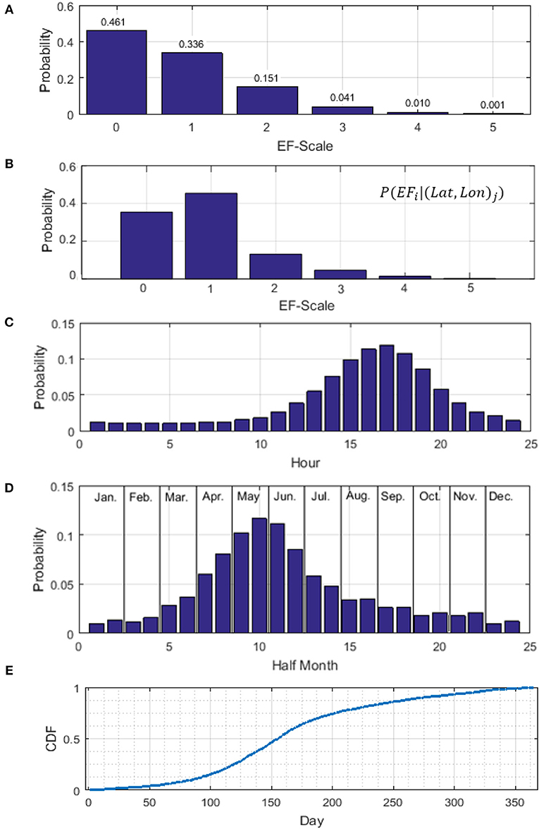
Figure 6. Probability density functions by (A) EF-scale for the contiguous United States, (B) EF-scale for a specific location in Oklahoma City; (C) spawn hour; (D) spawn month, and (E) cumulative probability distribution of tornado spawn day of the year.

Using the simulated tornado spawn location, the intensity of a tornado can then be sampled using a site specific PDF:

$\begin{array}{cc}{P}_{EFi,Locj}=\frac{P(E{F}_i\cap Lo{c}_j)}{{\displaystyle {\sum }_{m=0}^{5}P(E{F}_m\cap Lo{c}_j)}}=\frac{P\left({(Lat,Lon)}_j|B_i\right)\times P(B_i)}{{\displaystyle {\sum }_{m=0}^{5}P\left({(Lat,Lon)}_j|B_m\right)\times P(B_m)}}& (4)\end{array}$

Figure 6B shows an example site specific PDF determined using Equation 4 for a location in Oklahoma City. Note that while EF-0 tornadoes have the highest occurrence probability for the contiguous US (see Figure 6A), Figure 6B shows that EF-1 tornadoes are most likely to spawn in Oklahoma City. For each simulated tornado, a site specific PDF for EF-scale is produced and used to simulate the EF-scale of the tornado.

Similar procedures are applied to simulate the tornado spawn hour, spawn date/month, and heading angle. For determining the tornado spawn hour, B_i represents the tornado spawn hour in a day (1 to 24). Figure 6C shows the PDF for tornado spawn hour for the contiguous US. For the heading direction or angle, the data are grouped into eight equal bins with a 22.5-degree increment. For the spawn date and month, the data are divided into 24 groups with each month split into two segments, first half and second half of the month (Figure 6D). It should be noted that the first half of each month always contains 15 days and the second half of the month contains the remaining days of that month. After the tornado spawned month segment has been determined (i.e., early January, late January etc.), the spawn day number of the year (1–365) is sampled using the cumulative distribution function shown in Figure 6E, which is developed based the spawn dates of all tornadoes in the SPC database.

It has been shown that tornado path length (L) and path width (W) tend to increase with increasing tornado intensity (Brooks, 2004). Therefore, tornado path length and width are simulated according to the EF-scale. A more intense tornado tends to have a longer path length and wider path width than that of the weaker ones. Following the study by Brooks (2004), the tornado path lengths and maximum widths are modeled using the two-parameter Weibull distribution (Figures 7A,B). The cumulative distribution function of the Weibull distribution is:

$\begin{array}{cc}F\left(x\right)=1-exp[-{\left(x/c\right)}^d]& (5)\end{array}$

where c and d are the scale and shape parameters of the distribution. The fitted distribution parameters using maximum likelihood method for path length and path width grouped by EF-scale are shown in Table 2.

FIGURE 7

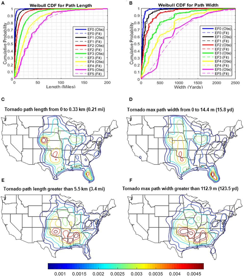
Figure 7. Observed and fitted cumulative distributions for path length (A); Observed and fitted cumulative distributions for path width (B); Small-scale tornado spawn location density contours for (C) length < 0.33 km, and (D) width < 14.4 m; large-scale tornado spawn location density contours for (E) length >5.5 km, and (F) width >112.9 m.

TABLE 2

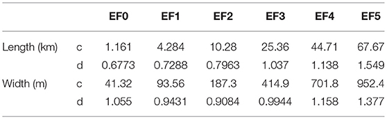
Table 2. Modeled Weibull distribution parameters for path length and path width by EF-scale.

To ensure that the tornado with and length follow both the statistical distribution and geographic features, the historical tornadoes are firstly grouped according to the EF scale. Then, EF-0 to EF-4 tornadoes are further divided into four different length (width) sub-group based on the 25th, 50th, and 75th percentiles. Since the data for EF-5 tornadoes are limited, the length and width of EF-5 tornadoes are split into two sub-groups, divided at the 50th percentile. These grouped dataset are used for generating the probability density contour maps using the KDE method. Tables 3, 4 show the grouping of path length and path width, respectively, based on quantiles and EF-scale. For instance, the subgroup L₂ in Table 3 for EF-2 tornado contains all tornadoes with path length that is in between 2.2 km and 6.5 km, which correspond to the 25th and 50th percentiles of the EF-2 tornado length.

TABLE 3

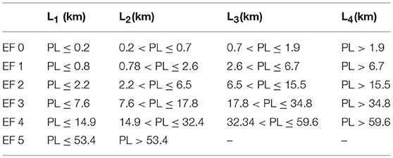
Table 3. Tornado length group, L_i.

TABLE 4

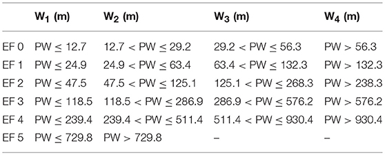
Table 4. Tornado width group, W_i.

The probability density contour maps conditioned on path length, P((Lat, Lon)_j |L_i), and path width, P((Lat, Lon)_j |W_i), are generated using the same approach used for other parameters such as EF-scale and spawn month. The KDE contour maps shown in Figures 7C,D reveal that small-scale tornadoes with lower 25th percentile path length [ ≤ 0.33 km (0.21 mi)] and path width [ ≤ 14.4 m (15.8 yd)] are often observed in Florida Peninsula, region along the Gulf coast and Central region of the US. Large-scale tornadoes with the path length and path width greater than the third quartile values [PL ≥ 5.5 km (3.4 mi) and PW ≥ 112.9 m (123.5 yard)] are more likely to spawn in Southeast region of the US (Figures 7E,F). Using the probability contour maps developed for each length and width subgroups, site specific probability density functions (PDFs) for path length and width grouped by quantiles are determined using Equations 3 and 4. Once the site specific PDFs for path length and path width have been determined, the inverse CDF method along with the fitted Weibull distribution parameters shown in Tables 3, 4 are utilized to simulate the tornado path length and width.

Wind Field Model

Wind field along the tornado length

Due to the difficulty of obtaining direct measurements of tornado wind speeds, the near surface wind speed is typically estimated based on the damage observed. A methodology to estimate the variation of tornado wind speed along its path using tree-fall and crop-fall patterns is developed (Rhee and Lombardo, 2018). The intensity of a tornado along the track usually degrades as the ground friction dissipates the energy of the tornado. After examined 150 tornado tracks, Twisdale and Dunn (1981) determined the intensity variation along the track of tornadoes. The fractions of the tornado strength for each of the highest EF-scales attained by a tornado are shown in Figure 8. In this study, it is assumed that the maximum intensity occurs at the middle of the tornado path and the lower bound EF-0 wind speed (65 mph) occurs at the fringe of the tornado track.

FIGURE 8

Figure 8. Tornado intensity variation along the track.

Wind field across the tornado width

The wind speed variation along the tornado width is modeled using the modified Rankine vortex model in which the tangential velocity can be computed as:

$\begin{array}{cc}{V}_{tan}\left(r\right)=\frac{r{\Gamma }_{\infty }}{\pi \left(r^2+r_c^2\right)}& (6)\end{array}$

where r is the radial coordinate with r = 0 at the center of the tornado vortex and r_c is the core radius where the maximum tangential velocity (V_{tan, max}) occurs, and V_tan,max is assumed to be uniformly distributed between the lower and upper bound wind speeds of the corresponding EF-scale. Γ_∞ = 2πr_cV_{tan, max} is the maximum vortex strength. Substitute Γ_∞ = 2πr_cV_{tan, max} into Equation (6) yields:

$\begin{array}{cc}{V}_{tan}\left(r\right)=\frac{r{\Gamma }_{\infty }}{\pi \left(r^2+r_c^2\right)}=\frac{2r\left(r_c{V}_{tan,max}\right)}{r^2+r_c^2}& (7)\end{array}$

Where the only unknown in Equation (7) is r_c. Collect the r_c terms in Equation (7) gives the following expression:

$\begin{array}{cc}{r}_c^2-\left(\frac{2r{V}_{tan,max}}{V_{tan}\left(r\right)}\right)r_c+r^2=0& (8)\end{array}$

Note that r_c is not equal to the maximum path width (W). According to the SPC database, the maximum path width is a damage based value and this study assumes that the building damage occurs when the tangential wind speed exceeds 65 mph (lower bound wind speed of an EF-0 tornado). Assume that the lower bound EF-0 occurs at the edge of the tornado path width, the core radius r_c can be determined by setting the tangential wind speed V_tan(r) = 105 km/h (65 mph.) at $r=\frac{W}{2}$:

$\begin{array}{cc}{r}_c^2-\left(\frac{W}{105kph}{V}_{tan,max}\right)r_c+{\left(\frac{W}{2}\right)}^{\text{}\text{}2}=0& (9)\end{array}$

The core radius is computed by substituting the simulated path width (W) and maximum tangential wind speed into Equation 9.

Synthetic Tornado Tracks Database and Applications

The developed computer program using the Matlab programming language is utilized to generate 1,000,000 years of synthetic tornadoes. The simulated database contains more than 1 billion simulated tornado tracks. To verify the applicability of the simulated tracks, comparisons are made between the simulated and observed tornadoes for EF-scale, spawn month, and spawn hour for various locations. In addition, using the catalog of simulated tornado tracks, a probabilistic tornado hazard analysis is performed for Moore, Oklahoma. To study the influence of domain size on tornado risk, tornado hazard curves for three different domain sizes are generated for a location in Moore, Oklahoma.

Tornado Tracks

As an illustrative example, comparison between the simulated and observed tornado tracks within a radius of 40 mi (64.4 km) from the Oklahoma City for an observation period of 43 years (1973 to 2015) is shown in Figure 9A. The full paths of the simulated tornadoes are shown in Figures 9B–D along with the EF-scale identified by color. The simulated tracks visually agree with the pattern of the historical tornado tracks. For instance, both the observe and simulated tracks show that EF-0 and EF-1 tornadoes tend to have shorter lengths when compared to the more intense EF-4 and EF-5 tornadoes. The corresponding tornado counts for each EF-scale are shown in Table 5, which match the historical counts reasonably well. Note that Table 5 shows the results for one realization over a 43-year time frame. The results may vary for different realization of 43-year time span.

FIGURE 9

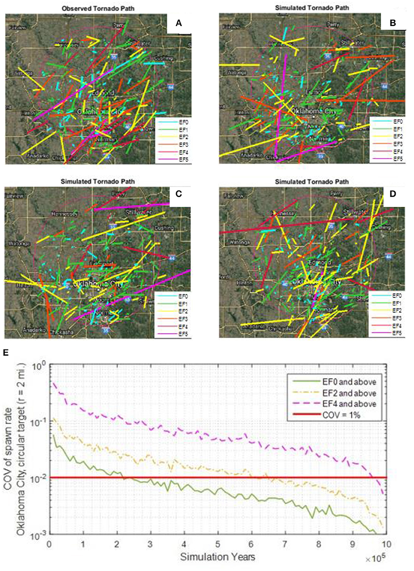
Figure 9. Tornado tracks for Oklahoma City, Oklahoma (A) actual observed tornado tracks from 1973 to 2015, and sample (B,C,D) tornado tracks for 43 simulation years; (E) convergence of spawn rate for Oklahoma City vs. simulation years.

TABLE 5

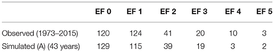
Table 5. Number of simulated and observed tornado tracks near Oklahoma City.

A previous study by Sigal et al. (2000) has shown that 100,000 simulation years may not be adequate to achieve stability of the simulated tornado hazard. A convergence study was carried out to determine the stability of the simulated occurrence rate for multiple realizations of 1 million simulated years for a 2-mile circular study domain located in Oklahoma City, Oklahoma. Figure 9E shows the convergence plot of the coefficient of variation (CoV) of the spawn rate vs. simulation year. It can be seen that about 200,000 simulation years are needed to keep the CoV of spawn rate of all tornadoes (i.e., EF0 and higher) to < 0.01. For intense tornadoes (EF4 and higher) that are more rare, slightly < 1 million simulation years are needed to maintain the CoV of spawn rate to < 0.01.

Tornado Intensity

The comparison between the simulated and observed tornado PDFs for the contiguous US by EF-scale are shown in Figure 10A. The breakdown of the simulated tornadoes by EF-scale matches the past observations very well, which confirms that the simulation program produces the correct ratios for different EF-scale tornadoes.

FIGURE 10

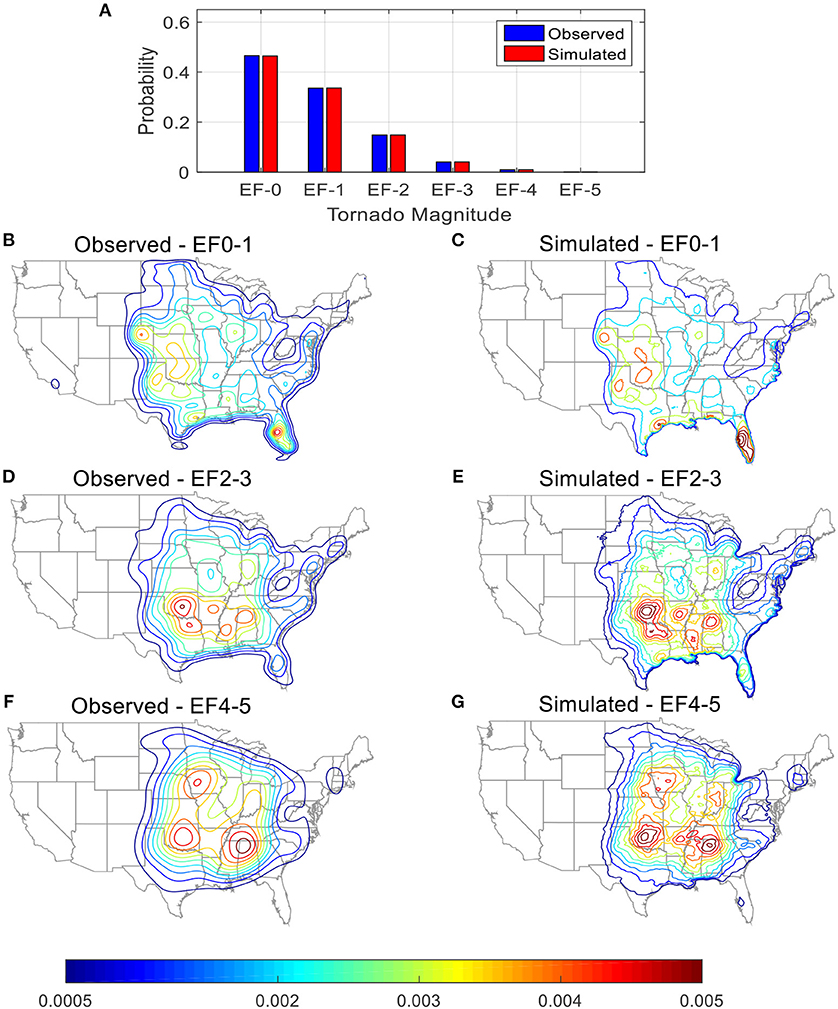
Figure 10. Comparison between observed and simulated tornadoes (A) spawn probabilities by EF-scale; probability density contours for (B,C) EF-0 and EF-1; (D,E) EF-2 and EF-3; (F,G) EF-4 and EF-5.

To confirm that the spatial distribution of tornado by EF-scale is properly capture in the simulated database, probability density maps are generated for simulated and observed tornadoes (Figures 10B–G). The patterns of the probability density contours of the simulated tornadoes for each EF-scale group match that of the contours from the observed tornadoes. Weak tornadoes (EF 0 and EF 1) have a wide spread area of occurrences and they cover the midsection and Southeast portions of the US. In addition, except for those occurred in the Tornado Alley, weak tornadoes are also likely to spawn in Florida peninsula and region around the Gulf coast. The high occurrences of weak tornadoes in the coastal regions are likely due to additional tornadoes that spawned during the landfall of tropical cyclones or hurricanes. Strong tornadoes (EF 2 and EF 3) have high probabilities of occurrence in the Southeast region of the US, which includes portion of the Tornado Alley and most of the Dixie Alley. The peaks of the probability density contours for major tornadoes (EF 4 and EF 5) are observed in Tornado Alley, Dixie Alley and Midwest.

Tornado Spawn Month

The seasonal variation of spawn probability of tornadoes is explicitly considered in this study. The comparison between the simulated and observed tornado monthly spawn rates is shown in Figure 11A. As can be seen, good agreements are achieved between the simulated and observed spawn probabilities for all 12 months.

FIGURE 11

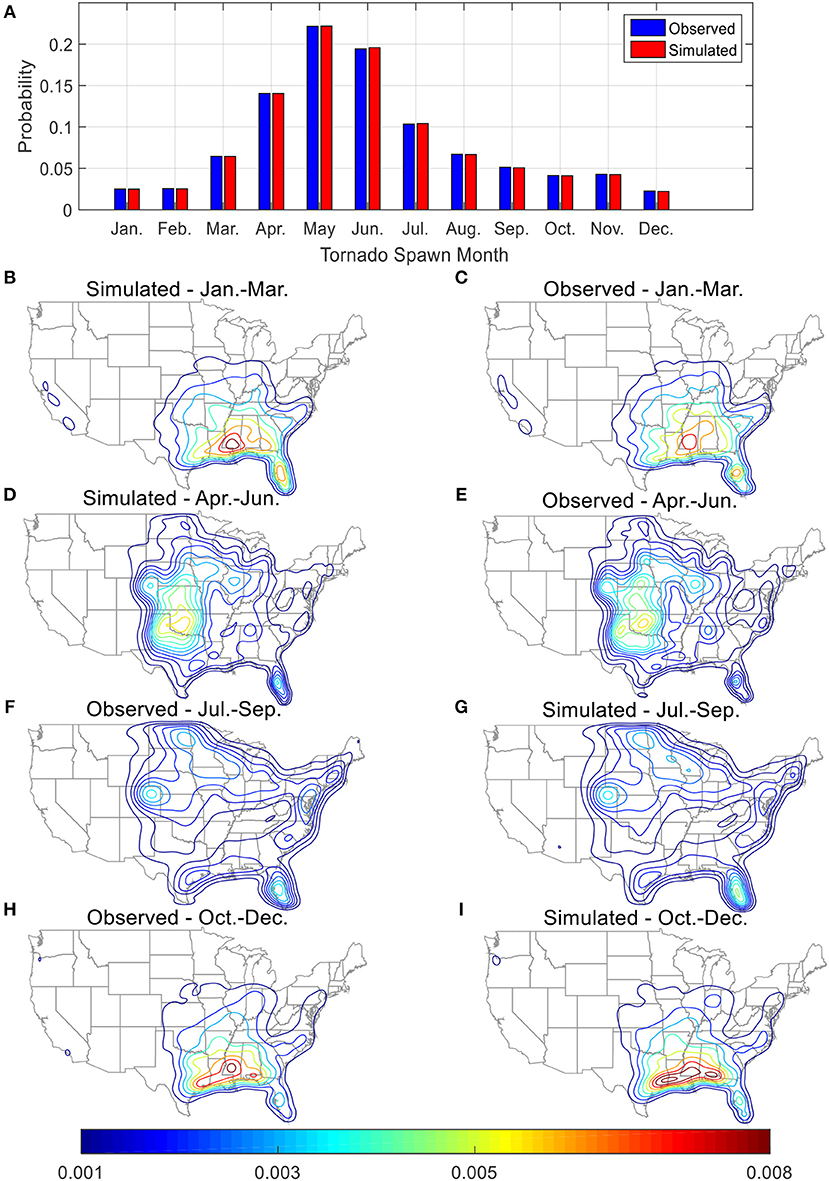
Figure 11. Comparison between observed and simulated tornadoes (A) spawn probabilities by month; probability density contours for (B,C) January to March, (D,E) April to June, (F,G) July to September, and (H,I) October to December.

Due to strong wind shears and atmospheric instability that often occurs in spring and summer, the months with high tornado spawn probabilities are April to July. The geographic and seasonal dependent behaviors of simulated tornadoes are shown in Figures 11B–I. The geographic regions with high spawn probabilities change drastically with the change of season. During the winter season (Figures 11B,C), tornadoes generally spawn in the Southeast region whereas during the summer (Figures 11F,G), tornadoes may spawn in the Mid-west and Northeastern part of the US.

Tornado Spawn Hour

It has been shown that tornado occurrence is highly correlated to the time or hour in a day. The occurrence density has been shown to closely follows the diurnal temperature curve (Kelly et al., 1978), with the peak occurrence probability during late afternoon, while minimum occurrence probability just prior to the sunrise (Figure 12A).

FIGURE 12

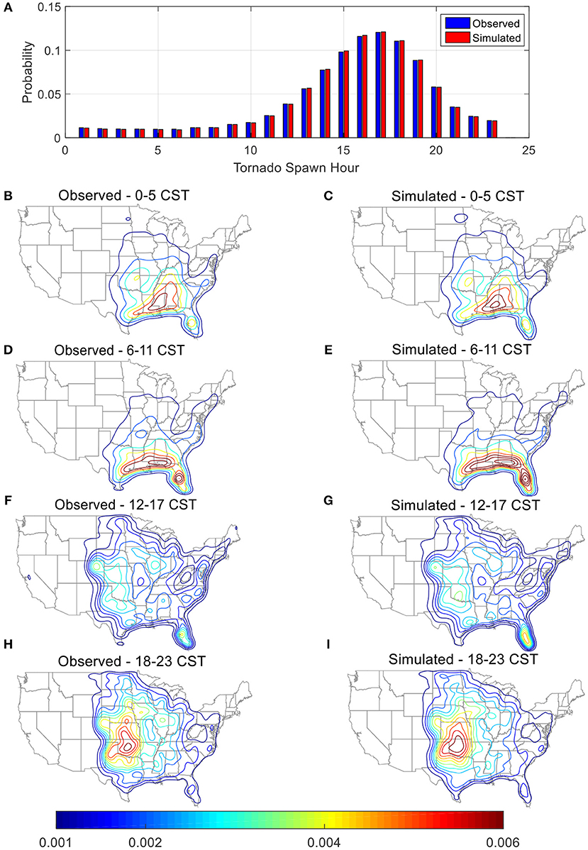
Figure 12. Comparison between observed and simulated tornadoes, (A) spawn probabilities by hour (CST); probability density contours for hours (B,C) 0–5; (D,E) 6–11; (F,G) 12–17; (H,I) 18–23.

The tornado spawn probability contours grouped by hour exhibit similar patterns as those grouped by month or season (Figure 11), which follow the diurnal temperature variation. When the diurnal temperature is low, between 6 am and 12 noon (CST), tornadoes are most likely spawn in Florida and along the Gulf Coast (Figures 12D,E). The peak spawn locations move to Midwest and further extend into the North and Northeast regions of the US between 12 noon and 11 pm (CST) (Figures 12F–I). Finally, the regions with peak occurrence probability return back to Florida, the Gulf Coast and Midwest areas between 12 mid night and 5 am (CST) (Figures 12B,C).

Comparisons for Select Cities

Comparisons are made between the simulated and observed statistics for tornado EF-scale, spawn month, and spawn hour for select cities. Four cities are chosen based on the degrees of tornado activity in the regions (Figure 13). These cities are: (1) Des Moines, Iowa (41.577, −93.617) located in High Plains region; (2) Oklahoma City, Oklahoma (35.457, −97.514) located in tornado alley; (3) Indianapolis, Indiana (39.777, −86.148) located in Midwest region; (4) Birmingham, Alabama (33.536, −86.798) located in Dixie alley. A search radius of 40 km (25 mi) from the city center is used to identify the tornadoes that affect the city of interest. Those tornadoes within the search radius are used to compare the statistics of the simulated and actual observed tornadoes.

FIGURE 13

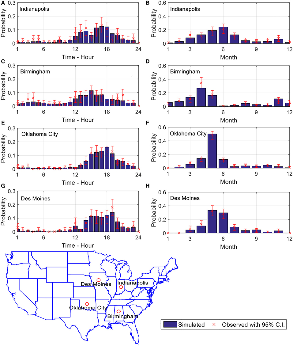
Figure 13. Probability density functions of tornado spawn hour and spawn month for (A,B) Indianapolis, Indiana; (C,D) Birmingham, Alabama; (E,F) Oklahoma City, Oklahoma; (G,H) Des Moines, Iowa.

Tornado Spawn Month and Time

The probability mass functions of tornado spawn hour and month for the select locations are shown in Figure 13. The red x marks are the means of the observed probability density values and the blue bars are the simulated probability densities. The 95% confidence intervals are plotted as red lines. It can be seen from Figure 13 that the probability densities of the simulated tornado spawn time and month match the observed data. All four cities considered experience elevated tornado activities from March to June. Past study have shown that, nocturnal tornado is the main reason that causes high fatality rate in the South-eastern region of the US (Ashley, 2007; Ashley et al., 2008). Unlike other cities which tornado often observed during the afternoon, Figures 13A,C show that Indianapolis and Birmingham have relatively high probabilities of observing tornadoes during the night.

Tornado Intensity

The annual tornado spawn frequencies within a radius of 40 km (25 mi) of the select cities for different EF-scales are plotted in Figure 14. The histograms show the simulated tornado frequencies and the x markers are the means annual frequencies of historical events. Also shown in Figure 14 are the 95% confidence intervals of the annual spawn rates estimated based on limited historical tornado events. The mean annual spawn frequencies by EF-scale of the simulated tracks fall within the 95% confidence intervals for all four cities. The numbers above the histogram are the mean number of simulated tornado tracks (top) and observed tornado tracks (bottom) for an observation period of 43 years. Note that there were no EF 5 tornado reported in Indianapolis and Des Moines over the record period (1950–2015); however, this does not mean the occurrence probability of EF 5 tornadoes in these cities are zero. Based on the simulation program, the model predicted annual spawn frequencies for EF-5 tornadoes in Indianapolis and Des Moines are 3.6 × 10⁻³ and 5.2 × 10⁻³ events per year, respectively. In other words, the mean return periods of EF-5 tornado for Indianapolis and Des Moines are 278 and 198 years, respectively.

FIGURE 14

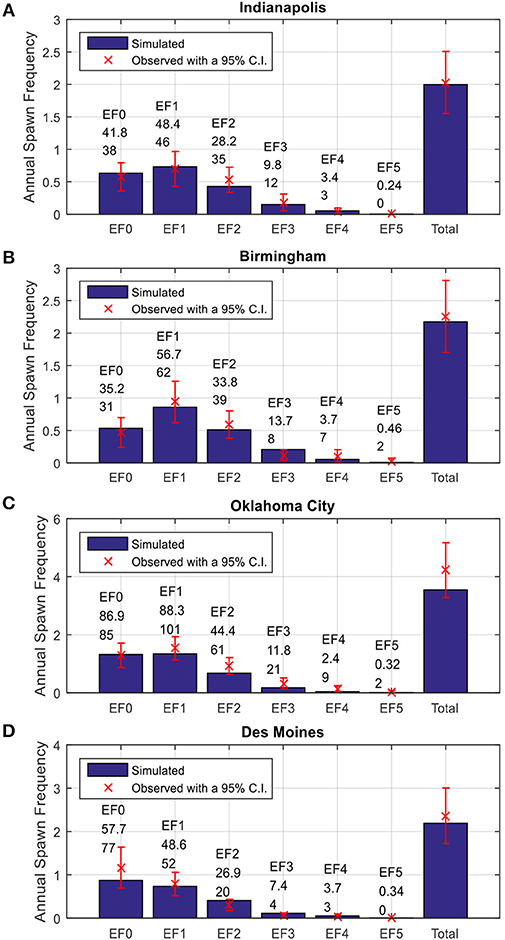
Figure 14. Annual spawn frequencies by EF-scale for (A) Indianapolis, Indiana (B) Birmingham, Alabama, (C) Oklahoma City, Oklahoma, and (D), Des Moines, Iowa.

Hazard Curves

To demonstrate one of the many potential applications of the simulated tornado database, tornado hazard curves in terms of 50-year exceedance probability vs. maximum wind speed are developed for Moore, Oklahoma for three different domain sizes (Figure 15). The maximum wind speeds occurred inside the domain are computed using the wind field model presented in section Wind Field Model. The radii of the three circular domains considered are 0.16 km (about 0.1 mi, small domain), 1.6 km (about 1 mi, medium domain), and 3.2 km (about 2 mi, large domain). All three domains are centered in Moore, Oklahoma and the study is aimed to assess the effect of domain size on tornado hazard curve.

FIGURE 15

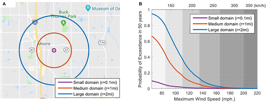
Figure 15. Domain sizes for (A) Moore, Oklahoma, and (B) 50 year tornado wind hazard curves.

The occurrence of tornado can be reasonably modeled using a Poisson process. The probability that the peak wind speed v_i is larger than a certain wind speed V induced by tornado during time period T can be described as:

$\begin{array}{cc}{P}_T\left(v_i>V\right)=1-exp\left(-\frac{n}{Y}T\right)& (10)\end{array}$

where n is the total number of tornadoes producing wind speed greater than the threshold value V inside the study domain. Y is the total number of simulation years (i.e., 1 million years in this study). T is taken as 50 years for 50-year hazard curve:

$\begin{array}{cc}{P}_{50}\left(v_i>V\right)=1-exp\left(-\frac{n}{Y}\times 50\right)& (11)\end{array}$

The 50-year hazard curves in Figure 15B show the domain size effect. The results indicate that the 50-year exceedance probability increases with increasing domain size and decreases with increasing peak wind speed. Based on the hazard curves shown in Figure 15, there is a 95% probability that the large domain with a 3.2 km (2 mi) radius area in Moore, Oklahoma will experience at least one EF-0 or stronger tornado with wind speed exceeding 105 km/h (65 mph) in a 50-year time span, whereas the small domain has about 9.8% chance of experiencing EF-0 or stronger tornadoes for the same 50-year time span. The hazard curves for various domain sizes may be used by engineers to design buildings and other structures to resist tornado loading with a prescribed safety level (exceedance probability).

Summary and Conclusion

In this study, the NOAA SPC tornado database is utilized to develop a stochastic simulation program. The spawn or touchdown locations are simulated using geographic dependent KDE, which specifically accounts for the spatial distribution of tornadoes properties at different geographic regions (e.g., tendency to spawn strong in Dixie alley and etc.). The simulated track parameters include the tornado occurrence rate, intensity (EF-scale), touchdown location, touchdown time, and path direction. All these parameters are geographic dependent, meaning the properties vary depend on the geographic locations. The simulated spawn rates and other parameters for the contiguous US and for four select cities are compared to observations and the modeled results compared well with the observed tornado records. As an illustrative example, the 50-year tornado hazard curves for Moore, Oklahoma with three domain sizes are generated using the simulated tornado database. The results show that domain size has a significant influence on the tornado hazard curve. Therefore, size effect (e.g., single-family vs. big box store) may need to be considered in building code for tornado design. The developed tornado database may be used by engineers for performance-based design or risk analysts for catastrophe modeling and loss estimation for tornado hazards.

Data Availability

Publicly available datasets were analyzed in this study. This datacan be found here: https://www.spc.noaa.gov/wcm/#data and https://www.spc.noaa.gov/wcm/#data<

Author Contributions

This work was a collaboration between the two authors. FF collected and analyzed the tornado data presented in this paper. WP guided and oversaw the development of the model and computer program.

Funding

The material presented in this paper is based on work supported in part by the US Forest Service Grant No. 16-DG-11083150-054. Any opinions, findings, and conclusions or recommendations expressed in this paper are those of the authors and do not necessarily reflect the views of the US Forest Service.

Conflict of Interest Statement

The authors declare that the research was conducted in the absence of any commercial or financial relationships that could be construed as a potential conflict of interest.

References

Ashley, W. S. (2007). Spatial and temporal analysis of tornado fatalities in the United States: 1880–2005. Weather Forecast. 22, 1214–1228. doi: 10.1175/2007WAF2007004.1

CrossRef Full Text | Google Scholar

Ashley, W. S., Krmenec, A. J., and Schwantes, R. (2008). Vulnerability due to nocturnal tornadoes. Weather Forecast. 23, 795–807. doi: 10.1175/2008WAF2222132.1

CrossRef Full Text | Google Scholar

Banik, S. S., Hong, H. P., and Kopp, G. A. (2008). Assessment of tornado hazard for spatially distributed systems in southern Ontario. J. Wind. Eng. Ind. Aerodyn. 96, 1376–1389. doi: 10.1016/j.jweia.2008.03.002

CrossRef Full Text | Google Scholar

Banik, S. S., Hong, H. P., and Kopp, G. A. (2012). Assessment of the wind hazard due to tornado outbreaks in southern Ontario. J. Wind. Eng. Ind. Aerodyn. 107–108, 28–35. doi: 10.1016/j.jweia.2012.03.003

CrossRef Full Text | Google Scholar

Boruff, B. J., Easoz, J. A., Jones, S. D., Landry, H. R., Mitchem, J. D., and Cutter, S. L. (2003). Tornado hazards in the United States. Clim. Res. 24, 103–117. doi: 10.3354/cr024103

CrossRef Full Text | Google Scholar

Botev, Z. I., Grotowski, J. F., and Kroese, D. P. (2010). Kernel density estimation via diffusion. Ann. Stat. 38, 2916–2957. doi: 10.1214/10-AOS799

CrossRef Full Text | Google Scholar

Brooks, H. E. (2004). On the relationship of tornado path length and width to intensity. Weather Forecast. 19, 310–319. doi: 10.1175/1520-0434(2004)019<0310:OTROTP>2.0.CO;2

CrossRef Full Text | Google Scholar

Brooks, H. E., Doswell, C. A., and Kay, M. P. (2003). Climatological estimates of local daily tornado probability for the United States. Weather Forecast. 18, 626–640. doi: 10.1175/1520-0434(2003)018<0626:CEOLDT>2.0.CO;2

CrossRef Full Text | Google Scholar

Daneshvaran, S., and Morden, R. E. (2007). Tornado risk analysis in the United States. J. Risk Finance. 8, 97–111. doi: 10.1108/15265940710732314

CrossRef Full Text | Google Scholar

Farney, T. J., and Dixon, P. G. (2014). Variability of tornado climatology across the continental United States. Int. J. Climatol. 35, 2993–3006. doi: 10.1002/joc.4188

CrossRef Full Text | Google Scholar

Kelly, D. L., Schaefer, J. T., and Mcnulty, R. P. (1978). An augmented tornado climatology. Mon. Weather Rev. 106, 1172–1183. doi: 10.1175/1520-0493(1978)106<1172:AATC>2.0.CO;2

CrossRef Full Text | Google Scholar

Meyer, C. L., Brooks, H., and Kay, M. (2002). “A hazard model for Tornado occurrence in the United States,” in 13th Symposium on Global Change and Climate Variations.

Google Scholar

Rhee, D. M., and Lombardo, F. T. (2018). Improved near-surface wind speed characterization using damage patterns. J. Wind. Eng. Ind. Aerodyn. 180, 288–297. doi: 10.1016/j.jweia.2018.07.017

CrossRef Full Text | Google Scholar

Schaefer, J. T., Kelly, D. L., and Abbey, R. F. (1986). A minimum assumptiontornado-hazard probability model. J. Clim. Appl. Meteorol. 25, 1934–1945.

Google Scholar

Sigal, B. M., Singhal, A., Pan, K., and Pasan, S. (2000). “Simulation of the tornado hazard in the U.S.,” in Proceedings of the 2000 Winter Simulation Conference (Orlando, FL), 1635–1644.

Google Scholar

Simmons, K. M., and Sutter, D. (2010). Economic and Societal Impact of Tornadoes. Chicago, IL: University of Chicago Press.

Google Scholar

Standohar-Alfano, C. D., and van de Lindt, J. W. (2015). Empirically based probabilistic tornado hazard analysis of the United States using 1973–2011 data. Nat. Hazards Rev. 16:4014013. doi: 10.1061/(ASCE)NH.1527-6996.0000138

CrossRef Full Text | Google Scholar

Standohar-Alfano, C. D., and van de Lindt, J. W. (2016). Tornado risk analysis for residential wood-frame roof damage across the United States. J. Struct. Eng. 142:4015099. doi: 10.1061/(ASCE)ST.1943-541X.0001353

CrossRef Full Text | Google Scholar

Strader, S. M., Pingel, T. J., and Ashley, W. S. (2016). A Monte Carlo model for estimating tornado impacts. Meteorol. Appl. 23, 269–281. doi: 10.1002/met.1552

CrossRef Full Text | Google Scholar

Suckling, P. W., and Ashley, W. S. (2006). Spatial and temporal characteristics of tornado path direction. Prof. Geogr. 58, 20–38. doi: 10.1111/j.1467-9272.2006.00509.x

CrossRef Full Text | Google Scholar

Tan, L., and Hong, H. P. (2010). Influence of spatial inhomogeneity of tornado occurrence on estimated tornado hazard. Can. J. Civil Eng. 37, 279–289. doi: 10.1139/L09-154

CrossRef Full Text | Google Scholar

Thom, H. C. S. (1963). Tornado probabilities. Mon. Weather Rev. 91, 730–736. doi: 10.1175/1520-0493(1963)091<0730:TP>2.3.CO;2

CrossRef Full Text | Google Scholar

Twisdale, L. A., and Dunn, W. L. (1981). Tornado Missile Simulation and Design Methodology. Palo Alto, CA: Electric Power Research Institute.

Google Scholar