Structural Health Monitoring of a Cable-Stayed Bridge Using Regularly Conducted Diagnostic Load Tests

Introduction

In order to ensure the structural integrity of a bridge throughout its life, it is essential that the structural components of the bridge are routinely inspected and evaluated. Inspections results and ensuing evaluations are used to classify the physical and functional condition of the bridge. The data generated from observational inspections are qualitative and rely on the inspector's experience, skill, and primarily focus on components of the bridge that can be readily seen. Other evaluation methods can be used, along with visual techniques, to improve the load rating process such as non-destructive evaluation technologies of bridge load testing. In a bridge load test, instruments such as strain gauges tilt meters, deflection devices, or other instruments are strategically located and attached to the bridge. A load, typically a heavily loaded vehicle, is then placed or driven across the bridge and the bridge response is measured.

Bridge load tests are often categorized into the categories of (1) proof tests, (2) diagnostic tests, and (3) in-service tests. Proof load tests are used in verifying the load carrying capacity of the bridge. A truck, weighing the load the bridge is intended to be able to carry safely, crosses the bridge. If the load crosses the bridge without damage and within the designated acceptable stress range, it was deemed as proof the bridge can carry the load. Diagnostic load tests are used to quantify a bridges response to heavy loads, and the response is then used to either directly evaluate the bridge or calibrate a numerical model which is in turn used to evaluate the bridge. In an in-service load test, instrumentation is used to measure the response of the bridge due to ambient traffic over a specified amount of time. Statistical analyses are then used to correlate the collected data to the traffic loading. In all of these different types of load tests, the response of the bridge to the load is used to determine an acceptable load rating for the bridge, and that rating is ultimately compared to the rating calculated using conventional methods.

The following publication provide both guidelines for using load tests to evaluate bridges as well as provide numerous applications (Pinjarkar et al., 1990; Fu and Tang, 1992; Moses et al., 1994; Lichtenstein, 1995; Nowak and Saraf, 1996; Chajes et al., 1997, 1999, 2000; Fu et al., 1997; NCHRP, 1998; The Institution of Civil Engineers, 1998; AASHTO, 2003; Chajes and Shenton, 2006; Schiff et al., 2006; Jeffrey et al., 2009; Hosteng and Phares, 2013; Olaszek et al., 2014; Peiris and Harik, 2016; Al-Khateeb et al., 2018). Most recently, Bayraktar et al. (2017), has employed static and dynamic field testing on a cable-stayed bridge.

Historically, bridges have undergone “one-off” load tests for specific reasons (i.e., low rating, damage, load carrying capacity validation, numerical model validation, assessment of repair effectiveness, lack of construction drawings, etc.) and have been instrumented with temporary sensors for a specific test. As such, there is little documented history of owners conducting a series of controlled load tests to quantify and monitor bridge health. This paper documents the initiation of a long-term monitoring program involving regularly conducted load tests used in combination with other long-term monitoring, all performed utilizing a comprehensive SHM system.

SHM has been a topic of intense research for some time; an early review of research in this area can be found in Doebling et al. (1996). The literature review was updated through 2001, in Sohn et al. (2003). Carden and Fanning (2004) also provided an updated review on vibration based SHM, picking up where Doebling et al. (1996) left off. More recent updates on SHM research include Das et al. (2016), Mesquita et al. (2016), and Seo et al. (2016). Finally, Li and Ou (2016) provide a detailed review of SHM of cable-stayed bridges which is particularly relevant here. Their paper includes a list of significant cable-stayed bridges that have installed on them SHM systems; many are located in Asia. The paper outlines the many uses for SHM data in the operation and maintenance of a cable-stayed bridge including the use of diagnostic load tests.

SHM systems have primarily been used for long-term in-service monitoring. In this paper, the focus is on demonstrating how SHM systems can make it possible to collect data during regularly performed diagnostic load tests.

Delaware's Indian River Inlet Bridge (IRIB), a cable-stayed bridge located in southern Delaware, has a permanent array of instruments that were installed in the form of a structural health monitoring system. Immediately after the IRIB was opened to traffic, a series of diagnostic load tests were conducted to establish the “healthy condition” or baseline behavior of the bridge. Additional diagnostic load tests or “physicals” have been conducted every 2 years to create an evolving “health record” for the bridge. To date, six load tests have been performed. This paper presents the methodology employed to build a comprehensive health record of the IRIB from biennial diagnostic load tests conducted utilizing the bridge's SHM system.

Description of the Cable-Stayed Bridge and the Structural Health Monitoring System

The following sections provide both details of the IRIB bridge and of the installed SHM system. More extensive descriptions can be found in Shenton et al. (2017a,b).

Cable-Stayed Bridge Description

The Charles W. Cullen Bridge at the Indian River Inlet, also called the Indian River Inlet Bridge (IRIB), is a 1,749 ft (533 m) long cable-stayed bridge with a 948 ft (289 m) main span and two 397 ft (121) m back spans. The bridge was designed using a combination of precast and cast-in-place reinforced concrete. The bridge is 105 ft (32 m) in width with two lanes of traffic and a shoulder in each direction. A 11 ft 9 ¾ in (3.6 m) wide pedestrian walkway is located on the east side of the bridge. This causes the centerline of the roadway to shift toward the west edge girder. The bridge is fixed at the north pylon but is free to expand at the south pylon and the abutments.

The deck is comprised of two edge girders, transverse floor beams spaced at 11 ft 9 ¾ in (3.6 m) on center, and a cast-in-place deck. The continuous cast-in-place edge girders are roughly rectangular in shape with dimensions of 5 ft 7/8 in (1.8 m deep) and 4 ft 11 in (1.5 m wide). The 8 ½ in (21.6 cm) thick cast-in-place deck has 1 5/8 in (4.13 cm) of latex modified concrete as a wearing surface. The bridge has two twin pylons that reach a height of 248 ft (75.6 m) above the ground. The pylons have a hollow box cross-section that is uniform below the deck level and above deck level tapers to the top of the pylon. There is a total of 152 stays, 38 per pylon. Nineteen stays emanate from each side of the pylons and are anchored to the edge girder on 24 ft (7.3 m) centers. The stay cables consist of seven wire strands in bundles of 19–61. The strands are waxed and encapsulated in high-density polyethylene sheathing. The stays are enclosed in a helical high-density polythene pipe with a raised helical strake to minimize the potential for wind-rain induced vibrations.

Construction of the bridge started in 2009 with the driving of the piles for the pylons. The bridge was opened to limited traffic in the winter of 2012 and was completed and opened to full traffic in May of 2012. Additional details of the bridge design and construction can be found in Delaware Department of Transportation (2019) and Nelson (2011).

Structural Health Monitoring System

The IRIB bridge was built with a fiber-optic SHM system installed throughout the full length of the bridge to monitor a variety of types of structural response. The system includes seven different types of sensors, with a total of 144 individual sensors installed on the bridge (Figure 1). The different sensors are designed to measure the structural response of the bridge under various environmental loads and live load conditions. They include:

• 70 strain sensors, located in the edge girders, pylons, and deck

• 44 accelerometers, mounted to the deck, pylons, and stay cables

• 9 tiltmeters mounted along the east edge girder

• 3 displacement sensors, one at each of the bridge expansion bearings (the two abutments and the south east pylon)

• 2 anemometers that measure wind speed and direction, one at deck level and one at the top of one pylon

• 16 chloride sensors in the deck in 10 locations

FIGURE 1

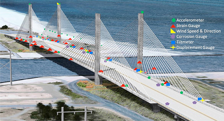
Figure 1. Layout of sensors in the SHM system.

All of the sensors are optical sensors, with the exception of the anemometers and 10 of the chloride sensors, which are conventional analog devices (Shenton et al., 2017a).

The SHM system operates 24/7. During operation two basic types of data are collected: “monitor” data and “event” data. Monitor data is collected continuously at both low and high frequency. For low frequency data, a single average sensor reading, computed from data taken at 125 Hz over a 10-min period, is recorded. For high frequency data, the data is continuously recorded at 25 Hz. The monitor data is used to quantify the response due to ambient live loads and well as to monitor long-term, gradual variations in bridge behavior. These long-term variations might be due to daily or seasonal thermal variations or slow degradation due to environmental effects or sustained load. In particular, ongoing data from SHM system is being used to evaluate long-term effects including cable forces (using cable vibrations), bearing condition (using bearing displacements), bridge ratings (using strain gauges), bridge deflections (using inclinometers), and thermal response (using multiple types of sensors). These applications have been outlined in Chajes et al. (2018).

Using a Series of Diagnostic Tests to Monitor Bridge Health

As mentioned, the SHM system is being used to monitor long-term response of the bridge due to ambient traffic and thermal changes/wind effects. However, none of this response data is due to controlled loads. While it would typically be very expensive to instrument and test a long-span bridge using controlled loads, even one time, by leveraging the existence of the permanent SHM system, it has become possible to conduct an ongoing series of controlled and calibrated diagnostic tests on the IRIB. While the predominant stresses long-span bridges come from dead loads, calibrated live load tests can be effectively used to assess change in bridge response and associated change in condition. In order to accurately and effectively evaluate the response of the bridge over time using the diagnostic load tests, a set of standard test procedures and the determination of the baseline response of the bridge that represents the “healthy” condition must first be determined. Doing this involves; (1) establishing a standard testing protocol, (2) establishing the baseline loading and baseline response, and (3) establishing key response parameters for future comparison.

Establishing Test Protocol

The determination of testing protocols takes place before any testing occurs. It involves, among other lesser details, determining the number of trucks to be used to load the bridge, their weight, the configurations (or passes) to be used to load the bridge, the number of passes, the timing of the test, and the required traffic control. Also included is whether the load passes will be static (stationary trucks or applied loads), pseudo-static (trucks moving at a slow crawl), or dynamic (trucks moving at full-speed).

Establishing Baseline Loading and Baseline Response

To establish the baseline loading and baseline response, a series of diagnostic load tests should be conducted a few months apart over the first year of service of the bridge. The first test should be conducted as close to the completion of bridge construction as possible. The remaining tests should be conducted when time dependent effects, such the increase in strength and stiffness of the concrete, concrete creep and shrinkage and associated pre-stressed losses, and any other ongoing changes that will affect bridge response, are believed to have stabilized. For some bridges this might take 6 months to a year after the bridge construction is completed. When comparing the response from these preliminary tests, one can look at both the nature of the time-history response due to the slowly moving truck loading or the magnitude of sensor data. While one should not expect perfect correlation, if the comparison of results from these initial tests are consistent and within an established variability of the data, the baseline test can be selected. The earliest test during which the bridge response is deemed to have stabilized will be selected as the baseline. While initial baseline tests may utilize a wide variety of load passes, based on evaluating the results from each pass, a baseline set of load passes should be determined. This baseline set of load passes should be the minimum number of passes that will yield comprehensive response results, and is called the “baseline loading.” The response resulting from the baseline loading is called the “baseline response.” The test for which these baseline results come is called the “baseline test.”

Establishing Key Parameters for Future Evaluation

While a large number and wide distribution of sensors may be needed to ensure that a comprehensive record of bridge response is captured, to simplify comparisons of future response to the baseline response, it is useful to identify a smaller number of key sensors for use in initial comparisons. If the comparisons indicate changes in response has occurred, the use of a more extensive set of sensors can then be employed. The key sensors will typically be those located at regions associated with maximum load effects. The key locations can be defined based on analytical results from the design process (such as locations that govern the load rating), as well as from the recorded response data from the initial load tests. At the key locations, both time histories and peak response resulting from various load passes can be used to make the initial evaluation of response compared to the baseline. For the IRIB bridge, the key sensors (see Figure 2) will be the strain gauges located on the west and east edge girder at midpsan (S-W7/8 and S-E7/8), at the controlling location (S-W21/22 and S-E21/22), as well as the strain gauge located in pylon 6 west just above the deck level (S-W24S). The controlling location is the longitudinal location along the edge girder that governs the bridge load rating. This happens to be at the quarter point of the backspan, and is within a few meters of strain gauges S-W21/22 and S-E21/22 (see Figure 2). The governing computed load rating is 1.17 (Al-Khateeb, 2016).

FIGURE 2

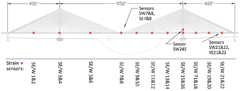
Figure 2. Key strain sensors on edge girder.

Other parameters that can be used to evaluate structural response are computed parameters such as the summation of girder strains across the bridge cross-section, load distribution factors, or girder neutral axis location. Which particular response parameters to use will depend on the specific bridge being evaluated.

Diagnostic Load Tests Conducted on the IRIB

The following sections describe the series of six diagnostic load tests that were conducted over the first 6 years of operation of the IRIB and used to both establish the baseline response and track the condition of the bridge over time.

Testing Protocol

A final testing protocol for how the load tests should be conducted and what passes should be included was determined after the initial three load tests were completed and evaluated. The final protocol included the minimum number of passes that should be conducted during each load test in order to assess bridge's condition. During several of the tests, extra passes were conducted to examine specific phenomena, however will not be discussed here as they were for independent focused research studies.

The final test protocol is comprised of 16 slow crawl passes. The first 12 passes involve single trucks traveling in one of the four travel lanes or one of the two shoulders. Next, two four truck passes involve trucks in a side-by-side formation traveling in the four travel lanes. Finally, two six truck passes involve trucks in a side-by-side formation across all six lanes (travel and shoulders). The pass number, pass identifier, truck formations, and direction of travel are given in Table 1 and pass configurations are shown in Figure 3. During the load tests, live loads are applied using up to six test trucks with a maximum combined weight of roughly 380 kips (1,690 kN). To minimize thermal effects during the testing period, all tests have been conducted at night, generally starting no earlier than 10 pm. This also minimizes traffic disruption. A complete load test report is submitted to DelDOT following each test.

TABLE 1

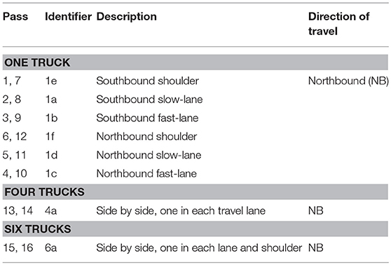
Table 1. Baseline loading.

FIGURE 3

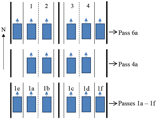
Figure 3. Truck configurations for baseline load passes.

Load Tests Conducted

Six diagnostic load tests have been conducted on the IRIB bridge since it was built. The initial test coincided with the opening of the bridge to full traffic. The next two tests were performed after 6 months of service and after 1 year of service (these three were used to establish the baseline). Following the initial three tests, ongoing tests have been conducted to provide response data at 2-year intervals. Thus, far, the 2, 4, and 6-years tests have been completed. DelDOT's plan is to continue conducting these biennial diagnostic tests as they will become increasingly valuable as the bridge ages. One important question that should be asked is whether the SHM system is robust enough to last years into the future when changes in bridge condition is much more likely to be seen. This is a very valid concern. To address this concern fiber optic sensors were selected as they are known for their excellent durability. Furthermore, the strain sensors are embedded in the concrete and this should increase the chances of their survival. Redundancy of sensor locations has been built into the system, and DelDOT is allocating ongoing funds to actively replaced sensors that have stopped working or don't have reliable measurements. There is also a plan to duplicate the key sensors by installing additional surface mounted sensors. However, until such long-term demonstration projects play out, we cannot know for sure that the systems will remain useable, and only by doing this can we learn how to design and implement SHM systems that will have long service lives.

Baseline Diagnostic Load Tests

As described, the first three load tests were all performed within the first year of service of the bridge and were used to establish the baseline response. Details of these three tests are summarized next.

Load test 1—April 30, 2012

In the first load test, conducted right before the bridge was fully opened to traffic, four trucks were used. The average truck weight was 63.5 kips (282 kN). A total of 17 passes were made in this first load test, 15 slow crawl passes and two dynamic passes. The first four passes were single truck passes and were all conducted using the same truck in each of the four travel lanes. Next, six passes were made with two trucks in specified formations. Finally, five passes were made in which all four trucks were placed in different formations. The dynamic, or high-speed, tests were conducted with all four trucks traveling at ~55 mph (88.5 km/h) with approximately a 100 ft. (30.5 m) interval between each truck.

Load test 2—November 28, 2012

After analyzing the results of the first load test, and reviewing the test procedures, a decision was made to add two more trucks in load test 2. By doing this all four travel lanes and both shoulders could be loaded simultaneously, thereby creating the maximum possible loading across the width of the bridge. The average truck weight for this test was 62.4 kips (282 kN).

A total of 25 passes were made in the second load test, 23 slow crawl passes and two dynamic passes. The first six passes were single truck passes in each of the four lanes and two shoulders. Next, eight two-truck passes were made in different formations and alignments. This was followed by two, three-truck passes, and then five four-truck passes. Finally, six trucks were used to make two passes in a side-by-side formation. The dynamic, or high-speed, tests were conducted with all four trucks traveling at ~55 mph (88.5 km/h) with approximately a 100 ft. (30.5 m) interval between each truck.

Load test 3—May 9, 2013

In the third load test, conducted 1 year after the bridge was fully opened to traffic, six trucks were used, with an average truck weight of 60.2 kips (268 kN). During this test, nine distinct pass configurations were used, and each pass configuration was repeated (repeatability of data is an important step in data validation). A total of 18 passes were made in the third load test, 16 slow crawl passes and two dynamic passes. The first 12 passes were single truck passes in each of the four lanes and two shoulders. Next, two four truck passes were made with the trucks in a side-by-side formation and two six-truck passes were made with the trucks in a side-by-side formation. Finally, the dynamic, or high-speed tests, were conducted with a single truck traveling at approximately 55 mph (88.5 km/h) in southbound slow lane.

Diagnostic Load Tests Used to Monitor the Bridge's Health

As described earlier, the next three load tests were performed at 2-year intervals. Details of these three tests are summarized next.

Load test 4—May 7, 2014

The fourth load test, conducted 2 years after the bridge was fully opened to traffic, was conducted following the standard test protocol with an average truck weight of 63.4 kips (282 kN). This test included additional passes with specific research objectives. In addition to the standard 16 slow crawl passes described in the protocol, there were also two dynamic, or high-speed, tests conducted with a single truck traveling at ~55 mph (88.5 km/h) in southbound slow lane. In addition, a couple of passes were conducted multiple times (six times) to assist in the quantification of measurement variability. Finally, at one point during the testing, the bridge was closed to traffic for 5 min and ambient measurements were taken to further assist in quantifying low-level sensor “noise.”

Load test 5—May 18, 2016

The fourth load test, conducted 4 years after the bridge was fully opened to traffic, was conducted following the standard test protocol with an average truck weight of 63.1 kips (281 kN). This test included additional passes with specific research objectives. In addition to the standard 16 slow crawl passes described in the protocol, this test included 10 additional passes. A total of 26 passes were conducted, 20 slow crawl passes and 6 dynamic passes. The first 18 passes were identical to the 16 included in protocol. To better assess the effect of the high-speed passes, dynamic passes were made of a single truck in the southbound shoulder, in the southbound fast-lane, in the northbound fast-lane, and in the northbound slow lane. Theses dynamic, or high-speed tests, were conducted with trucks traveling at approximately 55 mph (88.5 km/h). Finally, to simulate long trucks and their effect, additional passes were made using a two-truck train in the southbound slow-lane (twice), a three-truck train in the southbound slow-lane, and a four-truck train in the southbound slow-lane (all of these passes were conducted with the truck trains moving at a crawl speed).

Load test 6—June 6, 2018

Finally, the sixth load test, conducted 6 years after the bridge was fully opened to traffic, was identical to third load test (the standard 16 slow crawl passes described in the protocol plus two dynamic passes) with an average truck weight of 62.1 kips (276 kN).

Results

The following sections contain (1) a review the baseline response and associated response parameters that were established based on the first three load tests, (2) an evaluation as to how the response during the ensuing three load tests (years 2, 4, and 6) compares to the baseline response, and (3) a qualitative assessment as to how the response of the bridge has varied over time. Ongoing work is being conducted to determine at what level do individual changes in response, or a changing trend in response represent changes in bridge behavior. This work is aimed at establishing how severe a change in condition must be before the response parameters are “significantly” affected. Having data from this series of six tests has been very useful for the ongoing sensitivity evaluation.

Baseline Response

The baseline response was found from the three tests conducted within the first year of service of the bridge. From the second test (6 months) on, it was found that the bridge response stabilized. As such, the second load test was deemed to be the baseline test, and results from that test have been defined as the baseline results. The following will serve as a summary of those results.

Post-processing and Interpreting Data

Before looking at individual load test results, it is important to note that the same procedure was used to post-process test results from each test. For each sensor, the time-history record was first “zeroed” by taking the average of the first 25 data points and subtracting that value from the entire time history. In this way any initial offset in the record was eliminated. Next a moving average was computed using a window of 1.6 s (25 data points for data recorded at 15.6 Hz). This smoothing was performed to eliminate the inherent low-level noise in the sensor data. Finally, the maximum and minimum (i.e., peak) values of the record were determined.

When interpreting the results, it is important to note that strains, and associated stresses, with a positive value indicates tension. That means that maximum positive strains indicate the largest live-load tensile strain recorded and maximum negative strains indicate the largest live-load compression strain recorded. One should further note that having a live-load tensile strain/stress during the test does not necessarily mean that the element is in a state of net tension, as there can be a large initial compression component due to pre-stressing or post-tensioning that keeps the element in net compression. Where live load stress is reported, it is obtained by multiplying strain by Young's modulus of 29,000 ksi (200 GPa) for steel and 5,164 ksi (35.6 GPa) for concrete. For the concrete, the Young's modulus is based on an average compressive strength of 8,240 psi (56.8 MPa) determined from the tests of cylinders made during the concrete pours.

Baseline Peak Values

Table 2 shows the baseline peak strains for the key sensors for single, four, and six truck passes. For girder sensors, odd numbers indicate top sensors, where we will focus on peak negative values and even numbers indicate bottom sensors where we will focus on peak positive values. In the table, the peak positive values for the top sensors, and peak negative values for the bottom sensors are not shown as they are not significant compared to the other peaks. Gauge S-W24S is a pylon sensor and both positive (tension) and negative (compression) peaks are of similar magnitude and are both shown. The pass identifier for each peak value is given in parentheses.

TABLE 2

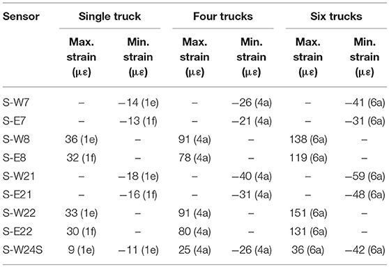
Table 2. Baseline response peak strain.

One can see that the west girder experiences larger strains than the east girder. This is because traffic is skewed toward that side of the bridge due to a wide pedestrian sidewalk on the east side of the bridge. This causes the centroid of the traffic lanes to be closer to the west girder. For the single truck passes, pass identifier (1e) produces the largest strains because that pass consists of a truck in the shoulder closest to the west girder.

In terms of the magnitude of peak strains, the very largest occurred during six side-by-side truck passes. The largest tension strain recorded during any of the load passes was 151 με at gauge S-W22. This gauge is located at the bottom of the western edge girder between pylon 6W and pier 7 (very close to the controlling location for load rating). The strain of 151 με corresponds to a live-load tensile stress in steel of 4.38 ksi (30.2 MPa) and a live-load tensile stress in concrete of 780 psi (5.38 MPa). The largest compression strain recorded during any of the load passes was −59 με at gauge S-W21. This gauge is located at the same location as gauge S-W22 (the controlling location), but is in the top face of the western edge girder. This strain corresponds to a live-load compression stress of 1.71 ksi (11.8 MPa) in steel and a live-load compression stress in concrete of 305 psi (2.10 MPa). The maximum tension and compression strains in the pylon recorded during any of the load passes were 36 με and −42 με, respectively. The strain of 36 με corresponds to a live-load tensile stress in steel of 1.04 ksi (7.17 MPa) and a live-load tensile stress in concrete of 184 psi (1.27 MPa). The strain of −42 με corresponds to a live-load compression stress of 1.21 ksi (8.34 MPa) in steel and a live-load compression stress in concrete of 215 psi (1.48 MPa). These pylon strains were recorded by strain gauge S-W24S (located in pylon 6 west just above the deck level).

Baseline Time Histories

Figure 4 shows the baseline time histories for the key strain gauges (S-W7 & SW-8, S-W21 & S-W22, and S-W24S) due to the six side-by-side truck pass. These time histories will be used later for comparison to load tests 4, 5, and 6. Please note that the plots of the time history are strain vs. time and not strain vs. distance. As such, the length of the plots varies depending on the exact velocity of the truck(s). Also note that the data recording always starts prior to any trucks coming onto the bridge, and so the first portion of the plot essentially measures ambient response and can be shortened as appropriate for plotting the results.

FIGURE 4

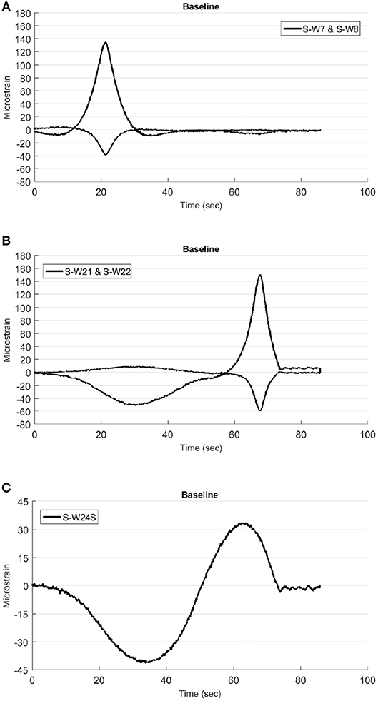
Figure 4. Baseline strain time histories for six truck pass: (A) midspan; (B) controlling location; (C) pylon.

Baseline Distribution Factors and Summation of Edge Girder Strains

Transverse load distribution is an important characteristic of a bridge and can be a useful quantity to track over time. The distribution factors for the IRIB were computed at midspan and at the controlling location based on one, four, and six loaded lanes. Table 3 shows the distribution factors that were computed at midspan and the controlling location.

TABLE 3

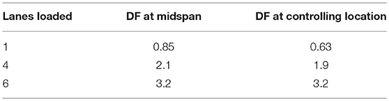
Table 3. Baseline response live load distribution factors.

To further improve the quantitative comparison, we can also look at the sum of the peak edge girder strains (top and bottom) at midspan (S-W7 + S-E7, S-W8 + S-E8) and at the controlling location (S-W21 + S-E21, S-W22 + S-E22). By using the sum of the two strains, some of the variability due to differences in transverse truck location can be eliminated. In a way, the sum of the peak strains is closely correlated to the total moment across the section at the two locations. Table 4 shows the summation of the girder strains at midspan and the controlling location.

TABLE 4

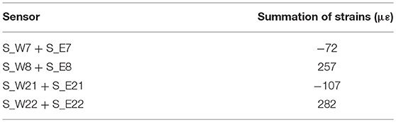
Table 4. Baseline response summation of girder strains.

It should be noted that we are not tracking distribution factors for the floor system as those members are not instrumented. It is believed that the very basic distribution between the two edge girders can be an indicator of change in behavior, perhaps due to changes in cable forces which are being monitored using cable vibrations as part of the SHM long-term monitoring effort.

Sensor Variability

In comparing results of “duplicate” passes, it is important to quantify the variability in the sensor readings that can come from (1) variations in truck location for duplicate passes, (2) bridge vibrations even in relatively low winds, and (3) general sensor noise related to sensor resolution. To establish this, (1) data can be collected for several minutes while no traffic is on the bridge and the wind is calm, and (2) several replicates of specific truck passes can be conducted. To accomplish this for the IRIB, traffic was stopped for 5 min and no cars or trucks were permitted to cross the bridge while data was recorded at 125 Hz (the test was conducted at night in calm wind conditions). In addition, six replicates of both a single truck pass (Pass 1e) and six side-by-side truck passes (Pass 6a) were conducted. By analyzing the results from these two series of tests, the threshold for a meaningful difference between measured strain values from different tests but from similar passes was found to be ± 4 με. This value can be used when evaluating the results from successive diagnostic load tests. Additional details regarding its determination can be found in Aloupis et al. (2019).

Bridge Response Compared to Baseline

In the following sections, the recorded response of the IRIB bridge during tests conducted at 2 years (load test 4), 4 years (load test 5), and 6 years (load test 6) after the bridge was opened to traffic are evaluated by comparing them to the baseline response. While it would not be expected that significant changes in condition and associated response would be noticed this early in the life of the structure, these test results represent the beginning of the “medical file” for the bridge (as if the bridge were a person undergoing biennial physicals). In fact, the bridge remains in excellent “health” as evidenced by the data about to be shown, and also as evidenced by the biennial inspection reports on the bridge. As noted in section Sensor Variability, variability between tests and due to sensor accuracy should lead to a strain variability of ±4 με. A very valid question is what level of change in strain is needed to signal a change in condition? This is an active area of ongoing research by the research team both for strain data due to diagnostic tests as well as all sensor data due to long-term ambient monitoring. Clearly the nature and location of the change in condition will how much the measured strain will change. By repeating the test every 2 years, both one-time changes and trending changes can be captured. It is anticipated that changes that follow a trend will be the best signals of bridge condition change. Finally, it is important to note that for all results presented, the response has been normalized to the loading magnitude of the baseline test.

Comparison of Time Histories

Figure 5 shows a comparison of the time history response of the key strain gauges at midspan (S-W7/8), the controlling location (S-W21/22), and in the pylon (S-24S). One can see that qualitatively, the response from test to test is very consistent. The peaks show some variation, but no trend of increasing nor decreasing magnitude is clear. In the next section, the specific values of the peaks will be investigated.

FIGURE 5

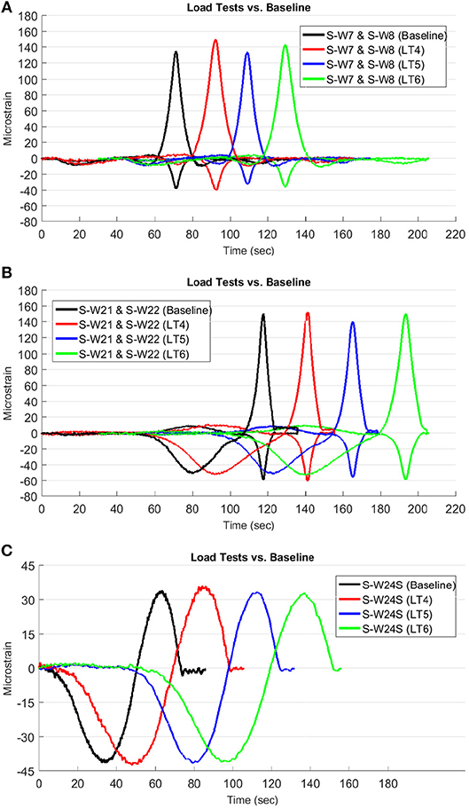
Figure 5. Baseline strain time histories compared to time histories from load tests 4, 5, and 6 for six truck pass: (A) west girder midspan; (B) west girder controlling location; (C) pylon.

Comparison of Peak Values

Table 5 presents a comparison of the peak strains recorded by key sensors during load tests 4, 5, and 6 to the baseline strains. Of the 30 differences from the baseline that were computed, 24 were <10%. Taking the absolute value of all 30 differences, the average difference is 6.5%. Furthermore, while there is no apparent trend in strain data, if any slight trend exists, it is for the peak strains to be getting smaller over time. Compared to the baseline, only one of the ten peak strain values during load test 6 was larger than the baseline value. In Figures 6, 7, one can graphically see how the peak strains have varied over time in comparison to the baseline value (the horizontal lines in the plots). This visual representation of the peak values shows that the ongoing response is quite similar to the baseline response, and with no discernable pattern of change.

TABLE 5

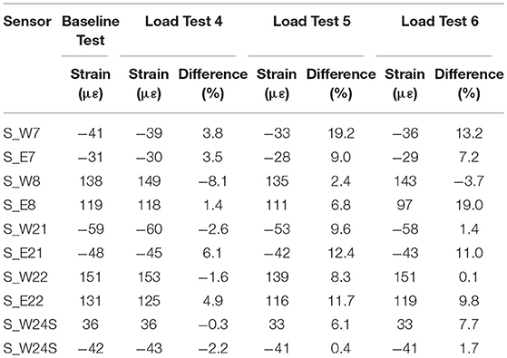
Table 5. Comparison of peak baseline strain for key sensors to peak strains for load tests 4, 5, and 6 for six truck passes.

FIGURE 6

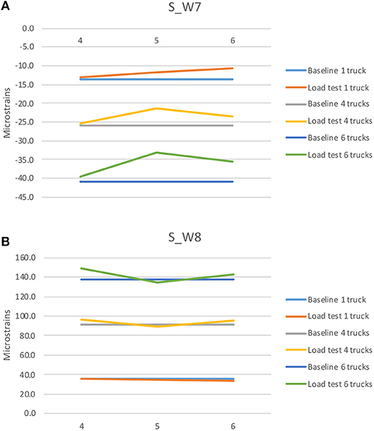
Figure 6. Peak strains at midspan from load tests 4, 5, and 6 compared to the baseline value: (A) top of west edge girder; (B) bottom of west edge girder.

FIGURE 7

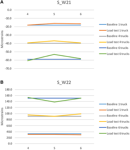
Figure 7. Peak strains at the controlling location from load tests 4, 5, and 6 compared to the baseline value: (A) top of west edge girder; (B) bottom of west edge girder.

Comparison of Distribution Factors and Summation of Edge Girder Strains

As mentioned earlier, both transverse load distribution factors and summation of top and bottom edge girder strains (east and west) can be useful parameters to track over time.

Table 6 provides a comparison of single, four, and six lane loaded distribution factors from load tests 4, 5, and 6 as compared to the baseline values. Of the 18 differences that were computed (absolute values), 10 were below five percent and all were below 10%. Using the absolute value of all 18 differences, the average difference is 4.5%. Table 7 shows the summation of top and bottom edge girder strain gauges at midspan for load tests 4, 5, and 6 as compared to the baseline value. Of the 12 differences that were computed (absolute values), nine were below ten percent and all were below 15 percent. Using the absolute value of all 12 differences, the average difference is 6.4%. If any minor trend is noted, it is that the summation of strains is getting smaller over time. Figure 8 shows graphically how the summation of strains have varied over time.

TABLE 6

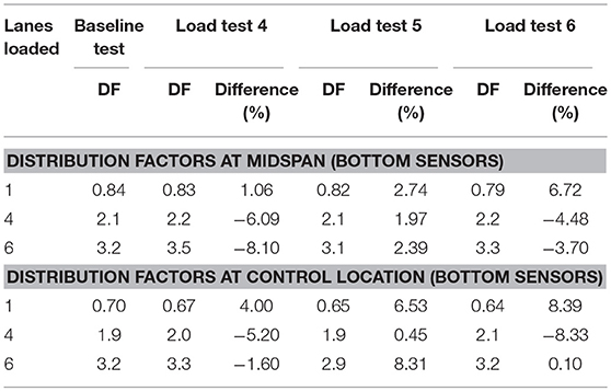
Table 6. Baseline distribution factors at midspan and controlling location compared to distribution factors from load tests 4, 5, and 6.

TABLE 7

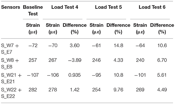
Table 7. Comparison of baseline summation of peak top and bottom girder strains at midspan and the controlling location to summation of peak top and bottom girder strains from load tests 4, 5, and 6 for six truck passes.

FIGURE 8

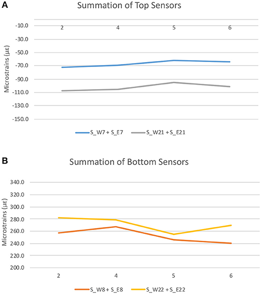
Figure 8. Summation of west and east peak strains: (A) top of edge girders at midspan and controlling location; (B) bottom of edge girders at midspan and controlling location.

Summary of Comparisons

The comparisons of time histories, peak values, and distribution factors all indicate that the bridge condition has remained unchanged during the first 6 years of service. While this is what would be expected, the database of response will be extremely valuable in the years to come. This data does contain variability, but absent trends in the data, suggest that future variability within the ranges seen here should be of no concern. On the other hand, trends in the data, or variability beyond what has been documented, would be cause for further investigation.

Conclusions and Future Work

This paper has described how SHM systems can be utilized to facilitate ongoing bridge health monitoring using regularly performed diagnostic load tests. The process involves first establishing a baseline response and then comparing future response to that baseline. In essence, the series of tests is analogous to a series of “physical exams” and together they create a “health record” for the bridge. The baseline response represents the “healthy” condition of the structure, and each successive test adds valuable information to record with which the change in condition and associated health of the structure can be assessed.

In the case of the IRIB, three diagnostic load tests were conducted to establish the baseline response of the bridge, and three additional diagnostic load tests (physical exams) have been conducted at 2-year intervals to create a health record for the bridge. The results indicate that the bridge is performing as expected. While some variability in response is observed, no defined pattern or trend in the response over time is evident. Future tests will be added to the health record (which also included visual inspection result), thereby enabling the owner to develop a more quantitative measure of the bridge's condition.

Should some event occur or condition arise in the future that raises concern about the health of the bridge, a load test can be quickly and easily conducted, and the results used in conjunction with visual inspection and theoretical analyses to fully assess the condition of the bridge. This becomes just one more tool in the engineer's toolbox for evaluating the bridge in such an instance.

The work presented shows how a bridge SHM system can provide value to a bridge owner. In addition to (ideally) providing automatic early clues to potential problems, a periodic controlled load test can provide confirmation that conditions have not changed.

Future work will focus on developing a more detailed characterization of test-related variability of the response parameters and on determining when changes in response indicates actual structural change and is not simply due to expected test-related variability. The preliminary result of that effort are presented in Aloupis et al. (2019).

Author Contributions

HA-K, HS, and MC contributed to the conception and design of the study. HS was in charge of developing the SHM system, and oversaw all of the load tests. HA-K and CA performed the data analysis. HA-K, CA, and MC wrote portions of the first draft of the manuscript. All authors contributed to manuscript revision, and read and approved the submitted version.

Funding

The project was supported by funds from both the Delaware Department of Transportation and the Federal Highway Administration under grants BRDG422145–09001448, BRDG422158–TASK 30A−1717, BRDG422161–TASK 30B−1717, and BRDG422162–TASK 30C−1717.

Conflict of Interest Statement

HA-K was employed by the company Jacobs Engineering

The remaining authors declare that the research was conducted in the absence of any commercial or financial relationships that could be construed as a potential conflict of interest.

Acknowledgments

The authors would also like to acknowledge a number of individuals, agencies, and firms for their support and role in developing and implementing the structural health monitoring system for the Indian River Inlet Bridge and for their assistance in conducting the controlled load test. These include the Delaware Department of Transportation for the financial support to develop and implement the structural monitoring system, and for help during the load tests (Doug Robb, Craig Stevens, Marx Possible, David Gray, Alastair Probert, Jason Arndt, Craig Kursinski, Raymond Eskaros, and the crew from the southern district); the Federal Highway Administration for the financial support to develop and implement the structural monitoring system; Cleveland Electric Labs/Chandler Monitoring Systems (Jim Zammataro, Keith Chandler, Jennifer Chandler, and Abee Zeleke); and University of Delaware students for their help during the load tests and other activities (Pablo Marquez, Nakul Ramana, Jack Cardinal, and Patrick Carson).

References

AASHTO (2003). Manual for Condition Evaluation and Load and Resistance Factor Rating (LRFR) of Highway Bridges. Washington, DC: American Association of State Highway and Transportation Officials.

Al-Khateeb, H. T. (2016). Bridge Evaluation Utilizing Structural Health Monitoring Data. Ph.D. Dissertation, University of Delaware, Newark, DE.

Google Scholar

Al-Khateeb, H. T., Shenton, H. W III., H. W., Chajes, M. J., and Wenczel, G. (2018). Computing continuous load rating factors for bridges using structural health monitoring data. J. Civil Struct. Health Monitor 8, 721–735. doi: 10.1007/s13349-018-0313-4

CrossRef Full Text | Google Scholar

Aloupis, C., Chajes, M. J., and Shenton, H. W. (2019). “Quantification of uncertainties in diagnostic load test data,” in Proceedings of the Bridge Engineering Institute Conference (Honolulu, HI).

Google Scholar

Bayraktar, A., Turker, T., Tadla, J., Kursun, A., and Erdis, A. (2017). Static and dynamic field load testing of the long span nissibi cable-stayed bridge. Soil Dyn. Earthq. Eng. 94, 136–157. doi: 10.1016/j.soildyn.2017.01.019

CrossRef Full Text | Google Scholar

Carden, E. P., and Fanning, P. (2004). Vibration based condition monitoring: a review. Struct. Health Monitor 3, 355–377. doi: 10.1177/1475921704047500

CrossRef Full Text | Google Scholar

Chajes, M. J., Mertz, D. R., and Commander, B. (1997). Experimental load rating of a posted girder–and–slab bridge. J. Bridge Eng. 2, 1–10. doi: 10.1061/(ASCE)1084-0702(1997)2:1(1)

CrossRef Full Text | Google Scholar

Chajes, M. J., and Shenton, H. W. (2006). Using diagnostic load tests for accurate load rating of typical bridges. J. Bridge Struct. 2, 13–23. doi: 10.1080/15732480600730805

CrossRef Full Text | Google Scholar

Chajes, M. J., Shenton, H. W., Al-Khateeb, H. T., Wenczel, G., Natalicchio, C., Chen, J., et al. (2018). “Structural Health Monitoring of Delaware's Indian River Inlet Bridge,”in Proceedings of the International Bridge Conference (Washington, DC).

Google Scholar

Chajes, M. J., Shenton, H. W. III., and O'Shea, D. (2000). Bridge condition assessment and load rating using nondestructive evaluation methods. J. Transport. Res. Rec. 1696, 83–91. doi: 10.3141/1696-48

CrossRef Full Text | Google Scholar

Chajes, M. J., Shenton, H. W III., H. W., and O'Shea, D. (1999). “Use of field testing in delaware's bridge management program,” in Proceeding of the 8th International Bridge Management Conference, TRB, National Research Council (Denver, CO).

Google Scholar

Das, S., Saha, P., and Patro, S. K., (2016). Vibration-based damage detection techniques used for health monitoring of structures: a review. J. Civil Struct. Health Monitor 6, 447–507. doi: 10.1007/s13349-016-0168-5

CrossRef Full Text | Google Scholar

Delaware Department of Transportation (2019). Indian River Inlet Bridge. Available online at: https://www.deldot.gov/information/projects/indian_river_bridge/ (accessed January 1, 2019).

Doebling, S. W., Farrar, C. R., Prime, M. B., and Shevitz, D. W. (1996). Damage Identification and Health Monitoring of Structural and Mechanical Systems from Changes in Their Vibration Characteristics: A Literature Review. Los Alamos National Laboratory Report. LA-13070-MS, Los Alamos, NM.

Google Scholar

Fu, G., Pezze, F., and Alampalli, S. (1997). Diagnostic load testing for bridge load rating. J. Transport. Res. Rec. 1594, 125–133. doi: 10.3141/1594-13

CrossRef Full Text | Google Scholar

Fu, G., and Tang, J. (1992). Proof Load Formula for Highway Bridge Rating. Transport Research Record, 1371, Washington, DC.

Google Scholar

Hosteng, T., and Phares, B. (2013). “Demonstration of load rating capabilities through physical load testing: ida county bridge case study,” in Part of InTrans Project 12-444, Bridge Engineering Center. (Ames, IA: Iowa State University).

Google Scholar

Jeffrey, A., Breña, S. F., and Civjay, S. (2009). Evaluation of Bridge Performance and Rating through Nondestructive Load Testing. Amherst, MA: University of Massachusetts.

Google Scholar

Li, H., and Ou, J. P. (2016). The state of the art in structural health monitoring of cable-stayed bridges. J. Civil Struct. Health Monitor. 6, 43–67. doi: 10.1007/s13349-015-0115-x

CrossRef Full Text | Google Scholar

Lichtenstein, A. G. (1995). Bridge Rating Through Nondestructive Load Testing. Final Report, NCHRP Project 12-28A, Washington, DC.

Google Scholar

Mesquita, E., Antunes, P., Coelho, F., Andre, P., Andre, A., and Varum, H., (2016). Global overview on advances in structural health monitoring platforms. J. Civil Struct. Health Monitor. 6, 461–475. doi: 10.1007/s13349-016-0184-5

CrossRef Full Text | Google Scholar

Moses, F., Lebet, J. P., and Bez, R. (1994). Applications of field testing to bridge evaluation. J. Struct. Eng. ASCE 120, 1745–1762. doi: 10.1061/(ASCE)0733-9445(1994)120:6(1745)

CrossRef Full Text | Google Scholar

NCHRP (1998). Manual for Bridge Rating Through Load Testing. NCHRPProject l2-28 A, Transportation Research Board, Washington, DC.

Nelson, E. T. (2011) Indian River Inlet Bridge – Surviving the Storms. Chicago, IL: Aspire the Concrete Bridge Magazine, Precast/Prestressed Institute.

Google Scholar

Nowak, A. S., and Saraf, V. K. (1996). Load Testing of Bridges, Research Report UMCEE 96-10. Ann Arbor, MI: University of Michigan.

Google Scholar

Olaszek, P., Lagoda, M., and Casas, J. R. (2014). Diagnostic load testing and assessment of existing bridges: examples of application. Struct. Infrastruct. Eng. Mainten. Manag. Life-Cycle Design Perform. 10, 834–842. doi: 10.1080/15732479.2013.772212

CrossRef Full Text | Google Scholar

Peiris, A., and Harik, I. (2016). “Load testing of bridges for load rating,” in 7th International Conference on Sustainable Built Environment (Kandy).

Google Scholar

Pinjarkar, S. G., Guedelhoefer, O. C., Smith, B. J., and Kritzler, R. W. (1990). Nondestructive Load Testing for Evaluation and Rating. NCHRP Project 12-28 Final Report.

Google Scholar

Schiff, S. D., Piccirilli, J. J., Iser, C. M., and Anderson, K. J. (2006) Load Testing for Assessment Rating of Highway Bridges. Research Project No. 655, Clemson University, Clemson, SC.

Google Scholar

Seo, J., Hu, J. W., and Lee, J. (2016). Summary review of structural health monitoring applications for highway bridges. J. Perform Construct. Facilities 30:04015072. doi: 10.1061/(ASCE)CF.1943-5509.0000824

CrossRef Full Text | Google Scholar

Shenton, H. W. III, Al-Khateeb, H. T., Chajes, M. J., and Wenczel, G. (2017a) Indian river inlet bridge (Part A): description of the bridge the structural health monitoring system. Bridge Struct. 13, 3–13. doi: 10.3233/BRS-170111

CrossRef Full Text | Google Scholar

Shenton, H. W. III, Al-Khateeb, H. T., Chajes, M. J., Wenczel, G., Arndt, J., and Stevens, C. (2017b) Indian river inlet bridge (Part B): lessons learned from the design, installation operation of the structural health monitoring system. Bridge Struct. 13, 15–24. doi: 10.3233/BRS-170112

CrossRef Full Text | Google Scholar

Sohn, H., Farrar, C. R., Hemez, F. M., Shunk, D. D., Stimemates, D. W., and Nadler, B. R. (2003). A Review of Structural Health Monitoring Literature: 1996–2001. Los Alamos National Laboratory Report, LA-13976-MS, Los Alamos, NM.

Google Scholar

The Institution of Civil Engineers (1998). Guidelines for the Supplementary Load Testing of Bridges, The Institution of Civil Engineers, National Steering Committee for the Load Testing of Bridges. London: Thomas Telford Publications.