Measuring Structural Deformations in the Laboratory Environment Using Smartphones

Introduction

The demand for advanced engineering education in many universities makes the use of low-cost laboratory equipment a very attractive option, particularly in developing countries and remote colleges (Al-Habaibeh and Parkin, 2003). Fundamental components of laboratory equipment that are used to measure deformations of test-beds include mechanical dial gauges, strain gauges, and displacement sensors with supporting data acquisition systems. Displacement sensors such as linear variable differentiation transformers (LVDTs) and strain gauges usually require careful installation/calibration and data translation (Abdel-Jaber and Glisic, 2016), for example the conversion of volts/ohms to engineering units. Usually trained specialists are required to install sensors, increasing the overall cost of the measurement collection. Therefore, low-cost and easy to use sensor technologies with supporting software are promising alternatives for students, academics and researchers (Girolami et al., 2017).

Vision-based systems are non-contact and can be set at a certain distance from a structure (depending on the size of the structure, required measurement accuracy among other factors). Systems predominantly consist of one or more cameras and an operating system with image processing algorithms. Applications of vision-based systems in monitoring deformations of structures dates back to early 90 s, when Stephen et al. (1993) measured static and dynamic responses of the Humber Bridge. Since then numerous methods such as photogrammetry and digital image correlation have been developed and validated to accurately measure deformations of laboratory and real-world structures from image frames collected with high-resolution industrial cameras and user grade camcorders such as GoPro cameras (Choi et al., 2011; Ho et al., 2012; Brownjohn et al., 2017; Khuc and Catbas, 2017; Kromanis and Liang, 2018). Cameras with zoom lenses offer image collection of certain locations on structures from long distances (Ye et al., 2013; Feng and Feng, 2017). Frequently measured structural parameters include dynamic and static displacements and cracks in concrete structures (Adhikari et al., 2014). Substantial information about the theory underpinning image processing and case studies on deformation monitoring are summarized in recently published review papers (Brownjohn et al., 2017; Xu and Brownjohn, 2017).

Camcorders or professional cameras might not always be available, however almost every student, academic and researcher has a smartphone. Due to the economy of scale and use of smartphones on a global level, they can be acquired at a low-cost. Smartphones are equipped with powerful computer systems and high-resolution cameras, which allow capture of high quality images and videos. The increasing processing power and camera capabilities of smartphones make them a powerful measurement collection tool when integrated with appropriate applications (apps) (Nayeem and Want, 2014). Preliminary studies report applications of smartphones as a component for bridge monitoring systems. For example the incorporation of smartphone sensors such as the global navigation satellite systems tracking and integrated accelerometer to a monitoring system (Yu et al., 2015; McGetrick et al., 2017). Smartphone based object tracking apps have been proposed to dynamically collect structural displacements utilizing smartphone cameras (Min et al., 2015; Zhao et al., 2015). However, currently there is no freeware readily available for obtaining structural deformations from images collected of structures under loadings. The above examples make smartphones and free apps an attractive, low-cost option for deformation measuring of laboratory structures and educational activities. Free displacement analysis apps could be integrated into engineering and educational courses.

Smartphone technology is expected to improve even further, driven by phone companies providing more options and capabilities for their customers than ever before. Today some smartphones have the capability to record 4 k [3,840 × 2,160 pixel (px)] videos at 60 frames per second (fps) or even stereo vision for 3D reconstruction. Furthermore, when adding an optical zoom lens to a smartphone, deformation monitoring of full-scale bridges can be made possible. Kromanis and Al-Habaibeh (2017) obtained accurate movements of a pedestrian footbridge using a smartphone with a 20X zoom optical lens. The first natural frequency of the bridge as calculated from displacements obtained with vision-based technologies was in a good match to the frequency calculated from GNSS (Yu et al., 2014). A comparative study between high resolution and low-cost infrared vision systems has shown that equally good results can be obtained when considering appropriate analysis algorithms suggesting that with high resolution output even better results could be obtained (Shakmak and Al-Habaibeh, 2015). The studies of applications of smartphone technologies in long-term monitoring projects are not yet reported.

This study examines the performance of structural deformation monitoring using photos and videos collected with professional and smartphone cameras of beams subjected to static, dynamic and quasi-static loadings in the laboratory environment. Collected images/videos are analyzed with freeware and proprietary software. Obtained deformations are compared in terms of root mean square of deviation between selected measurement collection and image analysis methods. Results demonstrate that equally accurate structural responses can be obtained from contact sensors and images collected with professional and smartphone cameras, both analyzing images with freeware and proprietary software. A discussion is provided on the advantages, challenges, and benefits of using smartphone technologies over conventional measurement collection technologies, to measure deformations of structures in the laboratory environment.

Smartphone System for Measurement Collection

A schematic representation of a smartphone system for measuring structural response such as vertical deflections in the laboratory environment is provided in Figure 1. A cantilever beam is considered as a structure under loading. Artificial markers (or objects of interest) are drawn on its surface. The markers mimic structural features such as bolts in real-life structures. Structural deformations are determined from the location of markers, which are calculated using image processing software for each consecutively collected image or recorded video frame (further referred to as an image frame) while the beam is loaded. A smartphone is used to capture image frames of the deformation event. Marker locations are decided based upon required tasks and anticipated deformations. The load-response mechanism can also be used to assess the condition of the beam. For example, after an initial test the beam could be damaged and, once more, subjected to the same loading. Deflections in damaged and undamaged conditions could be compared for conditions assessment. Such a process could form a useful student activity in a taught structures course.

FIGURE 1

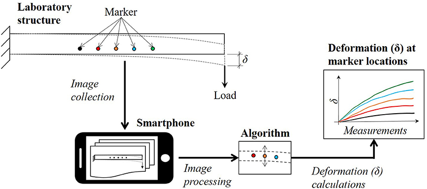
Figure 1. A schematic representation of measurement collection process of a structure under loadings using a smartphone.

The following sections describe processes underpinning image processing approaches for deformation calculations of structures, comparisons of selected algorithms with regard to the accuracy of deformation measuring of structures and a method that is used to evaluate the measurement accuracy between measurement.

Image Processing Approach and Techniques for Deformation Calculations

Collecting useful information from images/photographs has been research for more than a century. In some context, photogrammetry, which is a measurement technique used to determine the two- and three-dimensional geometry of objects from photographs, casts the foundation for many available image processing tools (Colwell, 1983). Photogrammetry has originated from the production of topographic maps (Hartley and Mundy, 1993). Developments of this technique have grown since the beginning of the technological era. Its expansion to video-processing shares considerable overlap in goals and algorithms with the computer vision (Hartley and Mundy, 1993) and has been implemented for deflection monitoring of bridge structures (Jiang et al., 2008). The fundamentals, however, of analyzing images of structures subjected to loadings and estimating their response remain the same.

Before images can be analyzed, there are some prerequisites that are influenced by the selected image processing algorithm and desired measurement accuracy. For example, camera calibration is a method of determining the intrinsic and extrinsic parameters of the camera used to record the structure motion, to remove lens distortion effects and to provide a conversion from pixel units to engineering units. There is a variety of approaches used to determine a scaling factor for converting pixels to physical distance. A pre-testing calibration method involves setting up the camera in the laboratory in an identical manner to that of the field test, i.e., focal length, angle etc. (Khuc and Catbas, 2017). The camera can be calibrated using the checkerboard pattern, which consists of white and black squares with known dimensions. Camera variables are used to remove lens distortion and provide a scaling factor for the image frames captured in the field trials. The scaling factor (SF) can be estimated as follows:

$\begin{array}{ll}SF=\frac{d}{D}=\frac{f}{p\times Z}& (1)\end{array}$

where d is a distance on the image, D is a known physical dimension, f is the focal length of the camera, p is the unit length of the camera sensor (mm/pixel) and Z is the distance from the camera to the monitoring location. A simpler method can also be used:

$\begin{array}{ll}SF=\frac{D_{known}}{I_{known}}& (2)\end{array}$

where D_known is the known physical length on the object surface and I_known is the corresponding pixel length on the image plane. Considering that the focus of this study is on the measurement collection of laboratory structures, Equation 2 is selected. It also should be noted that smartphone manufacturers have already embedded relevant algorithms to remove the lens distortion. The laboratory environment offers easy access to the structure, therefore a smartphone can directly (at no angle) face the structure (or the region of interests of the structure).

Figure 2 shows the image analysis process for deformation calculations. The process is initiated by choosing a reference image or image frame in a video. Preferably, this should be a clear image, in which there are no obstructions in front of the structure. The next step is to select a region of interest (ROI) which contains structural features such as corners, rivets or natural decay in a concrete or steel structure, physical features such as knots in timber beams or voids in concrete beams or artificially created features such as paint sprays. The listed features are referred to as structural features. This step can also be skipped, and structural features can be selected directly from the reference image. The step largely depends on the method that is considered for the extraction of mathematical features from the structural feature. Mathematical features, which could be edges, corners and blobs, characterize the structural feature. An analogy to a structural feature is a person's face. The nose, eyes, mouth and other face parts characterize the person's face. Once the structural feature is characterized, it can be located and tracked in other images.

FIGURE 2

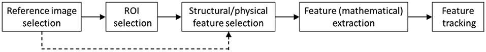
Figure 2. Diagram of image analysis process.

A range of factors govern the accuracy of measurement calculations from images. The computational complexity and resources are increased when real-time images are processed. In addition, the embedded artificial intelligence in an image processing algorithm can require high order of computation, hence, requiring even faster and more powerful computers to analyse real-time images. The focus of this study is on low-cost measurement collection systems and free/available image processing tools that can be used to obtain deformations of experimental setups in the laboratory environment.

Image Processing Algorithms

Three different image processing algorithms/software are considered and compared: (a) DeforMonit, developed at Nottingham Trent University (Kromanis and Al-Habaibeh, 2017), (b) QUB image processing method (further referred to as QUBDisp), developed at Queen's University Belfast (Del Rincon et al., 2018), and (c) “Video Gauge” (VG) software, a proprietary software built on a patented algorithm (Potter and Setchell, 2014). DeforMonit and QUBDisp are created using available Matlab algorithms. The aim is to demonstrate that comparable measurement accuracies can be obtained using the three image processing tools, hence, emphasizing the availability of low-cost vision-based technologies for measurement collection. These are especially attractive for educational institutions.

DeforMonit

DeforMonit is an app developed at Nottingham Trent University by R Kromanis. The app is a freeware which runs on Matlab platform, on Windows PCs. DeforMonit can be used to analyse both images and videos. At the current stage, it is designed to tracks locations of blob-like surface features (regions in an image that differs in properties such as brightness/color from surrounding regions), which are within a user's specified ROIs. The app does not have real-time capabilities, and image frames can only be analyzed after they are collected.

Image processing steps employed in DeforMonit are illustrated on an ROI drawn on a timber beam in Figure 3. ROIs of i^th image extracted from photos taken of the structure under loadings are converted to grayscale images and analyzed as matrices:

$\begin{array}{ll}{\text{U}}_{\text{i}}=\left[\begin{array}{c}{y}_{11}\cdots y_{1n}\\ ⋮\ddots ⋮\\ y_{p1}\cdots y_{pn}\end{array}\right]& (3)\end{array}$

y is a gray scale value for a pixel in p by n matrix U, where p and n is a row and column, respectively. The sharpness of ROIs is adjusted and the number of pixels is increased before they are converted to binary images. Binary images are analyzed for connected components—two or more pixels with the same color—black or white. The largest connected component (blob) in an image is the object of interest (marker). Local coordinates (x, y) for the marker are calculated for each ROI and converted to global coordinates (coordinates in the entire image not only in individual ROIs). Vertical, horizontal, and total movements of markers and strains generated from any two markers are calculated from the global coordinates. The location of the blob is calculated in the subsequent ROIs.

FIGURE 3

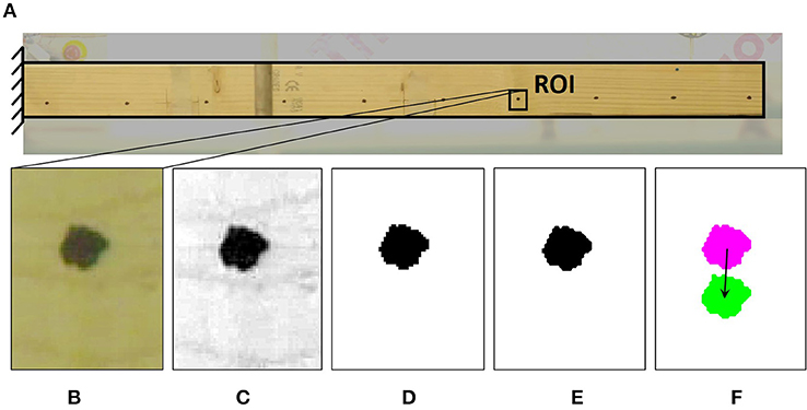
Figure 3. A ROI is selected on a timber beam (A). Image processing steps in DeforMonit for ROI (B): (C) convert ROI to a grayscale image, (D) create binary image, (E) leave only the largest blob and increase the image size, (F) calculate the location of the blob in each image.

VG Software

The Vision System originating from research at the University of Bristol (Macdonald et al., 1997) led to the VG software that was commercialized via the university spin-out Imetrum formed in 2003. For bridge displacement monitoring, high-resolution cameras equipped with long focal length lens are connected to the controller (computer) via Ethernet cables and a group of cameras are available for time-synchronized recording and real-time video processing in VG software.

In VG software, the target tracking algorithms used are correlation-based template matching and super resolution techniques which enable better than 1/100 pixel resolution at sample rates beyond 100 Hz in field applications. The tracking objects could be either artificial targets or existing features such as bolts and holes on bridge surface. The system supports exporting either two-dimensional displacement data via single-camera set-up or three-dimensional displacement information through multi-camera configuration. The VG software associated with the Imetrum hardware has been trialed by researchers in University of Exeter on several field tests. Results indicate that the system provides comparable sensing accuracy for deformation measurement as LVDT short-span bridge testing (Hester et al., 2017) and even better performance than GPS measurement in long-span bridge testing (Xu et al., 2017). In this study, video records by professional cameras or smartphones are imported to the VG software to extract ROI locations in the image plane which are then exported to convert to displacement information via a pre-defined scaling factor.

QUBDisp for Displacement Estimations

The processing framework of QUBDisp for displacement calculation is composed of three main blocks of motion pixel tracking (see Figure 2). A feature based approach is chosen due to being more reliable and robust than digital image correlation approaches (Hameed et al., 2009) and, when paired with a reliable feature extraction technique, with similar precision.

The feature extraction process selected for use in the algorithm is SURF (Bay et al., 2008) a robust and computationally inexpensive extension of SIFT (Lowe, 1999). The keypoints provided by SURF are scale and rotation invariant and are detected using a Haar wavelet approximation of the blob detector based on the Hessian determinant. These approximations are used in combination with integral images (the sum of pixel values in the image) to encode the distribution of pixel intensity values in the neighborhood of the detected feature. More on QUBDisp can be found in Del Rincon et al. (2018).

Once the points are detected, they must be tracked through subsequent frames to filter outliers and improve the displacement dynamic estimation. Careful application of threshold values must be maintained during this process, as features may become occluded or vary during the progression of images or a video. QUBDisp makes use of a Kanade-Lucas Tomasi (KLT) (Tomasi and Kanade, 1991) tracker to determine movement of the features detected. This method takes the points detected by the feature extractor and uses them as initialization values. The system removes outliers using the statistically robust M-estimator SAmple Consensus (MSAC) algorithm (Torr and Zisserman, 2000) which is a variant of the RANSAC algorithm. The MSAC algorithm scores inliers according to the fitness to the model and uses this together with a user-specified reprojection error distance to minimize the usage of outliers in the displacement calculation. Any features that do not meet these thresholds are rejected, with the inliers then tracked on the next video frame using the KLT algorithm. The displacement of the object is measured in pixels by calculating the relative movement between frames of the centroid of a matrix containing the extracted features.

Evaluation of Displacement Accuracy

The accuracy of the obtained/measured displacements are compared in terms of the root mean square (RMS) of deviation between two measurement collection methods such as DeforMonit and VG software. The first step is to find the RMS value of a vector (x) representing displacement measurements of i^th marker (x_RMS,Mi) over the observation period, in which n measurements are collected, which is calculated as follows:

$\begin{array}{ll}{x}_{RMS,M_i}=\sqrt{\frac{1}{n}{\sum }_{j=1}^n{x}_{j,M_i}}& (4)\end{array}$

In the next step, a vector of all x_RMS,Mi values is created and the RMS value of the selected measurement collection method (x_RMS,Method) such as DeforMonit is found using Equation 4. The RMS of deviation between two methods is a single positive number, which results from subtracting one x_RMS,Method value from another x_RMS,Method value. For example, the RMS of deviation between DeforMonit and VG software is |x_{RMS,DeforMonit} − x_{RMS,VG software} |.

Laboratory Tests

Three test scenarios are considered: (i) static, (ii) dynamic and (iii) quasi-static. Test specimens are set and monitored with contact sensors, cameras and smartphones in the structure's laboratory at NTU. Measurement collection technologies for the test set-ups are listed in Table 1. Motion pixels of selected markers drawn on the surface of test specimens are calculated using DeforMonit, VG software and QUBDisps. Real world displacements are estimated for static and quasi-static tests using Equation (2), in which a known dimension such as the depth of the beam is used. The accuracy of measured and/or calculated deflections are compared using RMS of deviation between all measurement collection methods.

TABLE 1

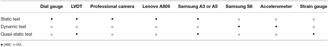
Table 1. Measurement collection technologies employed in the laboratory tests.

Static Test

In the static test a 45 mm wide, 70 mm high and 950 mm long timber beam is chosen. The beam is firmly fixed at its left end, thus making it a cantilever beam. Its setup and measurement collection systems are shown in Figure 4. Ten markers (M-i, i = 1,2, …, 10) are drawn on the surface of the beam. M-1 to M-10 are approximately 100 mm apart. Beam deformations are measured with three linear variable differentiation transformers (LVDT's) at the marker positions M5, M7, and M9 and one electronic dial gauge at M9. The load is applied manually by placing weight plates on a platform that is connected to the free end of the cantilever with a steel rod. The load steps are as follow: 0 N (self-weight of the weight platform), 100, 150, 170, 180, and 185 N. The load is removed taking off the weights as follows: 185 N (largest load), 180, 170, 150, 100, and 0 N. A professional camera (Sony FS7) and two phone cameras (Samsung A3 and Lenovo A806) are employed to capture images while the load is applied/removed.

FIGURE 4

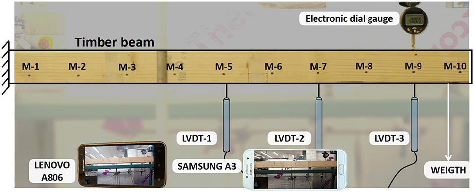
Figure 4. Static test set-up. Sony FS7 image.

Figure 4 shows an image captured with Sony camera, which is set 2 m from the beam. All markers are visible in an image frame to allow for collection of measurements of the entire beam. Sony camera captures 4,096 × 2,160 pixel images at 1 Hz. Samsung and Lenovo smartphones, which are placed closer to the beam, capture 4,128 × 2,322 pixel and 4,208 × 3,120 pixel images, respectively, at 0.5 Hz.

A deflection (δ_x) of a cantilever beam of a length (L) subjected to a point load (P) at its free end at a distance x from its support is calculated using Equation (5).

$\begin{array}{ll}{\delta }_x=\frac{P{x}^2}{6EI}(3L-x)& (5)\end{array}$

where E is the Young's modulus of the material and I is the second moment of area. According to Equation (5), the deformed shape of the cantilever is a parabola. Considering the laboratory setup described above, δ_x changes linearly with the change of the applied load. For example, if the beam rigidity (EI) is 6.2 × 10 Nmm², δ_@900mm at 100 N and 150 N loads is 4.26 and 6.4 mm, respectively, which is proportional to the increments of the applied load.

Time histories of vertical deformations of the cantilever measured with LVDTs and dial gauge are given in Figure 5A. The plot shows that deflections at specific locations are directly related to the applied load. For example, at LVDT-3 location the beam deforms approximately 46.5 μm/N. The vertical displacement plot of LVDT-3 reads 4.6 and 6.8 mm at 100 and 150 N loads, respectively. Vertical displacements obtained with image processing methods for markers that are close to LVDT locations are plotted in Figure 5B. Pixel motion values are multiplied by SF and converted to engineering units. The SF value is obtained by manually selecting a known distance, which for this test is the height of the beam close to M-8 location. All image analysis methods provide almost identical results and measurement variations are not discernible in the time-history plot shown in Figure 5B. A closer look at the vertical displacements of M-9 between 82 and 124 s, when 170 and 180 N are applied, show some measurement discrepancies between the three methods. DeforMonit does not remove outliers (QUBDisp employs outlier removal algorithm) or smooth measurements using a moving average filter, therefore some measurement noise remains in time histories. Displacements measured with LVDT-3 and dial gauge are plotted together with M-9 vertical displacements calculated from images collected with all cameras using DeforMonit (see Figure 5D). LVDT-3 measured displacements are slightly lower than those calculated using vision-based methods for periods when the load is applied. However, dial gauge measurements are the lowest for periods when the load is removed. This could be attributed to the load application mechanism and inertia force.

FIGURE 5

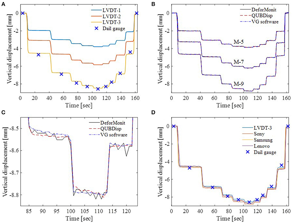
Figure 5. Vertical displacements of the beam: (A) measured with LVDTs and dial gauge, (B) calculated using all image processing methods for M-5, M-7, and M-9 from images collected with Sony camera, (C) a closer look at M-9 displacements from (B), and (D) measured with LVDT-3 and dial gauge and derived using DeforMonit for M-9 from images collected with all cameras.

M-1 to M-4 vertical displacements calculated with DeforMonit are analyzed to assess the camera performance against measurement accuracy of smartphones and the professional camera. Figure 6A shows M-1 to M-4 displacement time histories. Measurements from Sony camera are assumed to present reference measurement sets. Measurements from Lenovo are noisier than Samsung measurements. Statistical analysis of measurement errors between Sony and smartphones are given in Figure 6B. The error bar plot shows the difference between Sony and smartphones. Lenovo has much larger standard deviation values in comparison to Samsung for measurements obtained from all marker locations. This could be attributed to the quality of camera sensor, which is related to the price of the phone—Samsung A is more expensive than Lenovo A806.

FIGURE 6

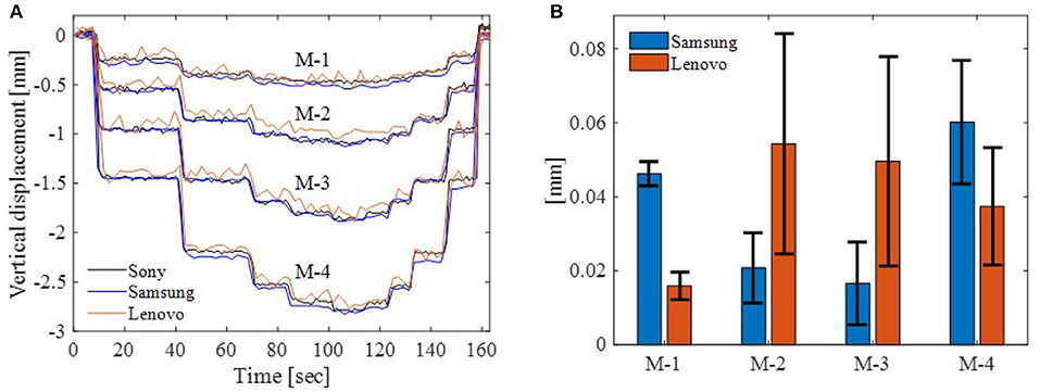
Figure 6. Vertical displacements of M-1 to M-4 derived using DeforMonit from images collected with all cameras (A). Statistical analysis of measurement accuracy from Samsung and Lenovo cameras (B).

RMS values of vertical displacements for all markers obtained using all image processing methods from images collected with Sony camera are very similar. RMS of deviations between vertical displacements collected with LVDTs and the dial gauge and calculated from images using three image processing methods are presented in Figure 7. The smallest RMS values are calculated from Lenovo images and LVDTs. Figure 5D shows that M-9 Lenovo displacements have smaller offset from LVDT-3 measurements than M-9 Sony and Samsung. This is also observed for other Lenovo and LVDT measurements (not shown in the plots). Deformations obtained from Sony and Samsung images are very close and less noisy than deformation estimated from Lenovo, which is the most noisy camera (see Figure 6A). RMS of the deviation between Sony and Samsung is the smallest. The difference between obtained displacements can be attributed to the selection of the scaling factor. One pixel in images collected with all cameras ranges from 0.224 to 0.238 mm. D_knownis the cantilever height. Its selection might be slightly different in all images, thus creating deviation in estimated displacements. This could be the reason why displacement values estimated from images collected with Lenovo for M-9 are closer to LVDT-3 measurements.

FIGURE 7

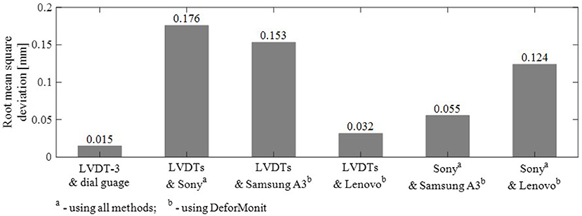
Figure 7. RMS of deviations between all measurement collection methods.

Dynamic Test

The beam that served for the static test is also used in the dynamic test. The length of the beam is increased to 1,000 mm. Dynamic properties of the cantilever are determined using a step-relocation method. In this measured input excitation method a load that is applied to a point of the structure is suddenly released (Farrar et al., 1999). In the dynamic load test (see Figure 8), a 200 N weight is applied 40 mm from the free end of the cantilever. The weight is connected to the cantilever with a cable tie. The cable tie is cut and the weight is suddenly dropped, exciting the cantilever. Beam accelerations are measured at 1,000 Hz with four uniaxial DeltaTron^® model 4,514 accelerometers placed on the top side of the beam (see Figure 8). A high frame rate (240 fps) video is recorded with Samsung S8 to evaluate the performance of the selected image processing methods.

FIGURE 8

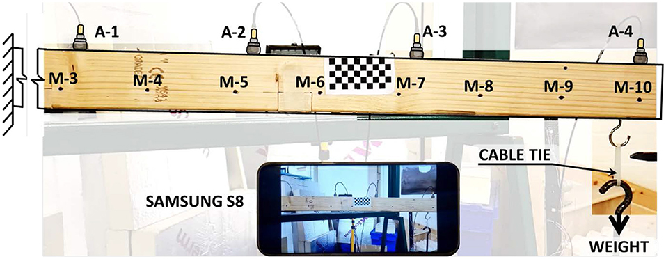
Figure 8. Dynamic test setup. Accelerations are monitored with four accelerometers (A-i, i = 1, 2, 3, 4).

Vertical displacements are estimated only using image processing therefore, displacement values are provided in pixels. Accelerations of accelerometer A-4 and vertical displacements of M-10 (estimated using VG software) are plotted in Figure 9A. VG software is selected as it is expected to provide the most accurate results. The wavelength of vertical displacements measured with accelerometer and calculated with VG software match. Similar results are obtained with other image processing methods. The first natural frequency (f) of the cantilever is found from the power spectral density (PSD) values. PSD signal is calculated using Welch's method, which is applied on detrended acceleration and vertical motion measurements. First natural frequencies found from A-4 and M-10 values are very close 30.64 and 30.59 Hz, respectively (see Figure 9B). A great advantage using vision-based technologies for collection of dynamic response is the ability to find frequencies at a range of locations on the structure. A plot of normalized PSD values with a fit line is shown in Figure 9C. The plot shows the mode shape of the test beam.

FIGURE 9

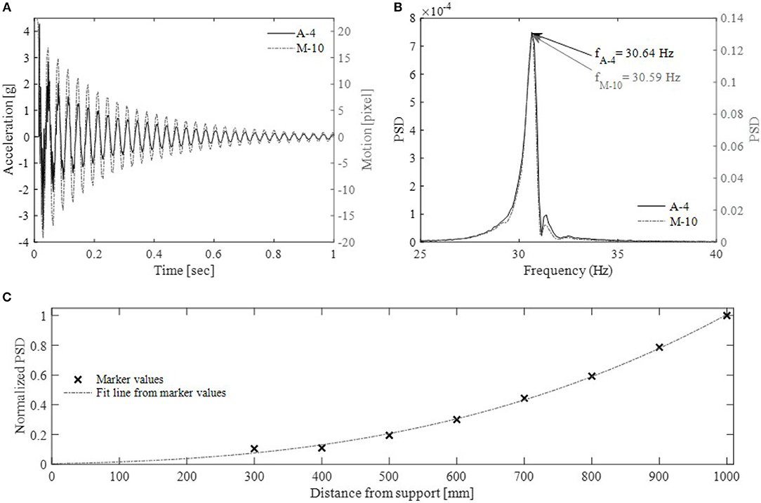
Figure 9. Dynamic test results: (A) accelerations collected with A-4 and vertical displacements of M-10 estimated using VG software, (B) power density spectrum of cantilever motion calculated from A-4 and M-10 value shown in (A,C) normalized PSD values for each marker locations with a fitted line.

All image processing methods perform well on the dynamic data sets. For the period shown in Figure 9A, the RMS of the deviation between vertical pixel values is:

• 0.005 pixel, between VG software and DeforMonit

• 0.158 pixel, between VG software and QUBDisp

• 0.163 pixel, between QUBDisp and DeforMonit

The first frequencies calculated from measurements of all four accelerometers are the same, 30.64 Hz. The first frequencies obtained using image processing methods range from 30.59 to 30.70 Hz. The average frequencies are as follows:

• VG software 30.59 Hz. f for all markers is 30.59 Hz,

• DeforMonit 30.63 Hz. f_M−6, f_M−7 and f_M−10 are 30.70 Hz, for other markers 30.59 Hz,

• QUBDisp 30.67 Hz. f_M−3 and f_M−6 are 30.58 Hz, for other markers 30.70 Hz.

Quasi-Static Test

An aluminum beam with width 8 mm, height 51 mm and length 800 mm is considered for the quasi-static tests. The right end of the beam is fixed and the left end is placed on a cylindrical support allowing for thermal movements. The friction between the bottom side of the beam and the top side of the support marginally affects the expansion/contraction of the beam, and therefore it is not considered in this study. The beam is instrumented with three LVDTs, two strain gauges (SGs) and four thermocouples (TCs). One thermocouple measures ambient temperature in the laboratory. Measurements from the named sensors in Figure 10 only are considered in the study. The location of sensors and test setup are shown in Figure 10. Daily temperature cycles are simulated using two 500 W infrared heaters. The heaters are placed 200 mm way and 100 mm above the beam and connected to the mains via a timer plug. LED lamp is installed close to the left end of the beam to cast light continuously on the region of interest, in which artificial markers are drawn. Samsung A5 smartphone is placed in a close proximity to the left end of the beam. Images are captured every 30 s. The test lasts 26:00 h. The temperature load schedule is shown and explained in Table 2.

FIGURE 10

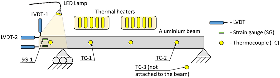
Figure 10. Quasi-static test set-up.

TABLE 2

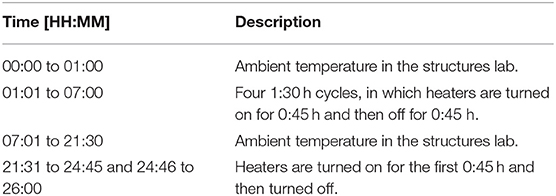
Table 2. Temperature load schedule.

Temperature histories are plotted in Figure 11A. TC-1 and TC-2 show simulated temperature cycles. TC-3 measures ambient temperature in the structures lab. 08:00 h from the beginning of monitoring (6:00 p.m. local time), there are no activities in the lab, and the central heating is turned off. This results in a gradual decrease of temperature until 20:00 h (6:00 a.m. local time), when heating is turned on. Fluctuations in TC-3 indicate activities in the lab. For example at 21:00 h the external gate to the laboratory is opened to receive deliveries creating a drop in ambient temperature. Strain time-history closely reflects temperature changes (see Figure 11B). When considering the third simulated temperature cycle (between 4:00 and 5:30 h), TC-1 measures temperature increase from 20 to 30°C. During this period, SG-1 measures 235 με increase in strain, which is a reasonable increase of material strain considering that linear thermal expansion of aluminum (α_Al) is between 21 × 10⁻⁶ m/mK and 24 × 10⁻⁶ m/mK. Horizontal and vertical displacements are provided in Figures 11C,D, respectively. Assuming that α_Al is 23.5 × 10⁻⁶ m/mK and temperature increases by 10°C, anticipated lateral and longitudinal expansions of the beam are 0.013 and 0.19, respectively. However, LVDT measurements do not provide expected results. Vertical (lateral) thermal movements of the beam (measured with LVDT-1) closely follow temperature changes, however, vertical displacements are much larger than calculated values. Longitudinal thermal movements poorly reflect temperature changes (see Figure 11D). Applied temperature affects the test setup/rig (surrounding environment), on which the beam is supported, hence resulting in complex thermal effects.

FIGURE 11

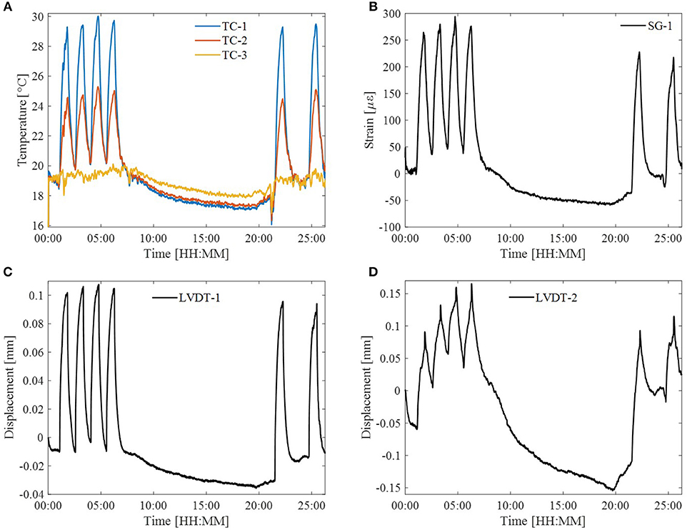
Figure 11. Time-histories of (A) temperatures, (B) strains and (C,D) displacements.

An image showing a part of the beam captured with the smartphone is shown in Figure 12A. The smartphone is located close to the beam resulting in a slight distortion of the image, see the top/bottom left corner of the beam. For this reason, raw (as captured) and undistorted images are analyzed using only DeforMonit. Camera parameters are obtained and applied to images, before they are analyzed. An undistorted image is shown in Figure 12B. When comparing raw and undistorted images, it can be seen that corners of the beam in the raw and undistorted images are rounded and stretched, respectively. Three artificial markers away from distorted image regions are selected for analysis.

FIGURE 12

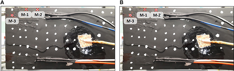
Figure 12. Raw (A) and undistorted (B) images of the left end of the aluminum beam. White spots are artificial markers. Three markers (M-i, i = 1, 2, 3) are selected for the displacement monitoring.

Vertical displacements of M-1 computed with DeforMonit from raw images are shown in Figure 13A. M-1 vertical displacements from raw and undistorted images are pre-processed using a moving average filter. Displacements between 0:50 and 7:30 h are shown in more detail in Figure 13B. RMS of deviation between measurements from raw and undistorted images for M-1 vertical displacements is 0.7 × 10⁻³ mm, which is 0.6% of the vertical displacement range. Recognizing that the difference between displacements is very small, the following analysis is carried out using raw images only.

FIGURE 13

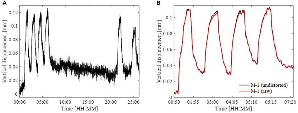
Figure 13. M-1 vertical displacements computed with DeforMonit from (A) raw images for the entire monitoring period and (B) undistorted and raw images from 0:50 to 7:30 h.

Raw vertical displacements of M-1 computed using all three image processing methods are plotted in Figure 14A. Displacements calculated with VG software and QUBDisp are less noisy than those computed with DeforMonit. Displacements computed with DeforMonit have a larger amplitude than displacements computed with other methods. Displacements computed with QUBDisp drift after 7:30 h and are different from displacements computed with DeforMonit and VG software. Pre-processed M-1 vertical displacements computed with all three methods and measured with LVDT-3 for the period between 0:50 and 7:30 h are shown in Figure 14B. Vertical displacement cycles measured with LVDT-3 are much larger than those obtained from image processing. VG software and DeforMonit calculated displacements follow similar patter, however, DeforMonit provides larger displacement values than VG software.

FIGURE 14

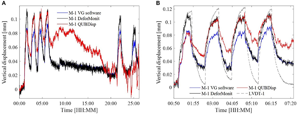
Figure 14. Vertical displacements (A) of M-1 for the entire monitoring period and (B) of M1 and LVDT-1 between 0:50 and 7:20 h.

Horizontal displacements obtained with LVDT-2 reflect both thermal response of the beam and temperature induced effects on the environment such as the test rig where the beam is set up. Figure 15 shows displacements for M-3 estimated using all image processing methods and measured with LVDT-2. A typical range of horizontal movements for a simulated cycle as obtained with image processing methods are 0.04 and 0.06 mm. QUBDisp and VG software produce very similar results for the first 5 h of the test. Later QUBDisp displacements begin to deviate from VG software results. DeforMonit calculated displacements follow closely VG software results, however peaks during the high temperatures are more amplified. An interesting observation is that LVDT-2 shows contraction of the beam when the temperature reduces slowly between 7:00 h and 20:00 h (see Figure 11A), however, image processing methods find the horizontal displacement to increase over this period.

FIGURE 15

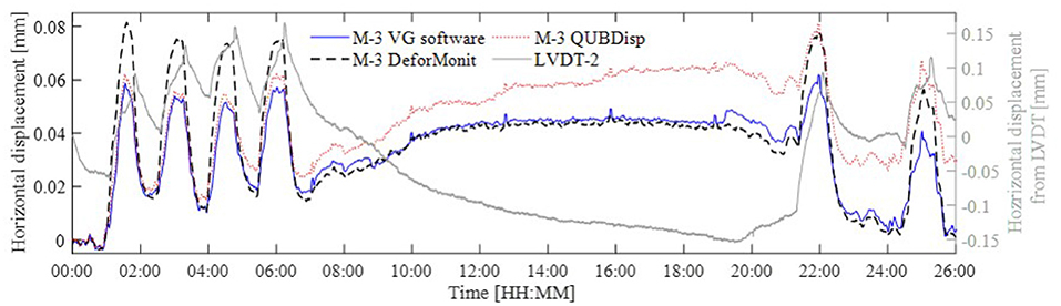
Figure 15. Horizontal displacements of M-3 and LVDT-2.

The change of a vector length between two markers over the original vector length between the same markers [further referred to as pixel strains (ε)] is calculated as follows:

$\begin{array}{ll}{\epsilon }_{M-l,M-k}=\frac{\sqrt{{(x_{M-l,1}-x_{M-k,1})}^2+{(y_{M-l,1}-y_{M-k,1})}^2}-\sqrt{{(x_{M-l,i}-x_{M-k,i})}^2+{(y_{M-l,i}-y_{M-k,i})}^2}}{\sqrt{{(x_{M-l,1}-x_{M-k,1})}^2+{(y_{M-l,1}-y_{M-k,1})}^2}}& (6)\end{array}$

where x and y are coordinates of two markers M − l and M − k at the 1st and i^th measurements. ε_M−1,M−2 and strain histories of SG-1 are plotted in Figure 16. Pixel strains are much larger than strains obtained from the foil strain gauge. Strains calculated from marker coordinates from DeforMonit and VG software are generally similar, although strain peaks during the simulations of temperature cycles vary in magnitude.

FIGURE 16

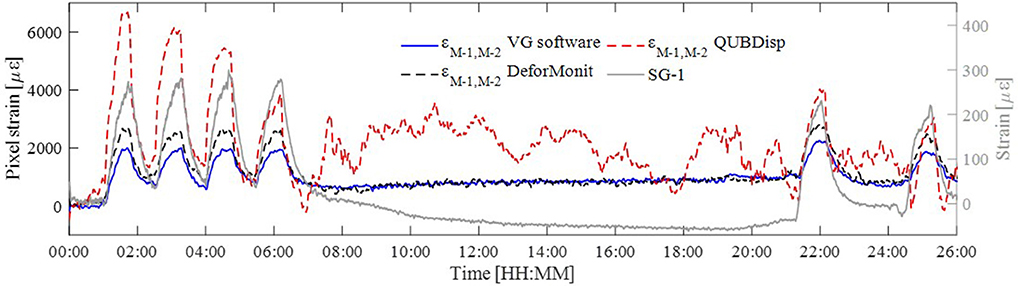
Figure 16. ε_M−1,M−2 and strain measured with SG-1.

RMS of deviations between image processing approaches and contact sensor measurements are not provided for this experimental setup. Deviations between all measurement collection methods are clearly discernible. LVDT-2 measured displacements are larger than the anticipated vertical displacements. This can be attributed to the complexity of thermal effects and their influence on the entire test setup. The best match between contact and vision-based measurements is for vertical displacements (see Figure 14B). It is also important to take into account that thermal response for this test setup is much smaller than static and dynamic response of the timber setup beam. For example a 0.1 mm change in vertical displacement is actually 4 pixels, and 2,000 με (from pixel) is equivalent to 0.002 pixel. The strain phenomenon, especially for thermal response, has to be researched in more detail. If strain range is 235 με it is a challenging task to obtain such a high resolution from images. On average the frame size of a 12 MP image is 4,200 × 2,800 pixel (width × height). If considering that a distance between two markers is 4,000 pixels, then to obtain a 235 με change the accuracy of 4000 × 235 × 10⁻⁶ = 0.94 pixel is required.

Discussion

Response measurements of three laboratory setups are obtained using contact sensors and analyzing image frames collected with smartphones and a professional camera. Image frames are then analyzed using a freeware (DeforMonit), free algorithm (QUBDisp) and proprietary software (VG software). Overall, when analyzing images collected with smartphone, a very good correlation of the different methods is obtained.

Images of static tests are captured with a professional camera Sony FS7, and then compared with data collected from Samsung A3 and Lenovo A803 smartphones. The Sony camera with an adequate lens used for the collection of image in the test costs around £7,000, whilst both phones cost no more than £200,- each. Plots in Figure 5 show that the smartphone technology with suitable software can provide a simple low-cost option to estimate deformations of laboratory structures. Deformations estimated with freeware (DeforMonit) and free algorithm (QUBDisp) agree well with LVDT and dial gauge measurements and are very similar to results obtained from the expensive proprietary software (VG software).

The dynamic test, in which the beam is excited by a sudden release of applied weight, can be easily performed in the laboratory environment, and to obtain a range of modes the weight can be dropped from different locations on the structure. When selecting less stiff structures than the beam in this study, tapping the surface of the structure with a hammer could also provide the required excitation. For example, vertical movements of less than five pixels can be detected (see Figure 6A). Measurements collected with accelerometers and estimated from a high frame rate video are very similar. The difference between the first natural frequency obtained with contact sensors and from the video is just under 0.2% [(30.64Hz − 30.59Hz) ÷ 30.64Hz × 100%]. Today some smartphones can boost a 240 fps video up to 960 fps, however the boost lasts only for 0.3 s and it is not easily controllable. Therefore, today from a 240 fps video the highest detectible frequency can go up to 120 Hz.

When analyzing quasi-static tests results, LVDTs provide displacements that are difficult to interpret. The entire lab setup is affected by changing temperature. Vertical displacements obtained using image processing methods are close to those measured with LVDT. Reliable results are obtained from the strain gauge, but when finding pixel strains from images, strain values are ten times higher than those measured with the strain gauge. However, trends of strain signals are very similar. This could be attributed to camera lens parameters, though results from undistorted images are almost the same as from raw images, or a difference between expansion of the aluminum section and the paint on the top surface of the beam. Quasi-static experiments can be coupled with a thermal imaging camera to obtain detailed information of applied temperature (Kromanis and Kripakaran, 2017).

Applications of smartphone technologies for estimations of deformations in the laboratory environment were proven to be successful. Smartphones are much easier to set up and use in comparison to contact sensors such as LVDTs and accelerometers, which need special connection (clamps or glued connections), have wires, need data acquisition units and sometimes technicians' help. If engineering units are required, then using the correct scale factor in image processing is important. Also installing a LVDT with its aperture perpendicular in two planes to the measured surface is challenging. DeforMonit and QUBDisp at the moment do not offer real-time measurement collection. VG software with appropriate hardware can be used in real-time tracking multiple targets simultaneously. It needs video frames at the first 2 s for training tracking parameters. A series of images for measurement should be converted to specific video files before they can be imported to VG software for post-processing.

All three image processing methods showed almost the same results in static and dynamic tests. However, there were slight deviations in estimated structural response for the quasi-static setup, in which VG software provided better results than DeforMonit and QUBDisp. The above discussions are summarized in Table 3. The table lists all technologies, next to which a qualitative evaluation based on their capability of providing accurate measurements for each test are provided together with their implementation costs. These are qualitative observations based on authors' opinions and test results.

TABLE 3

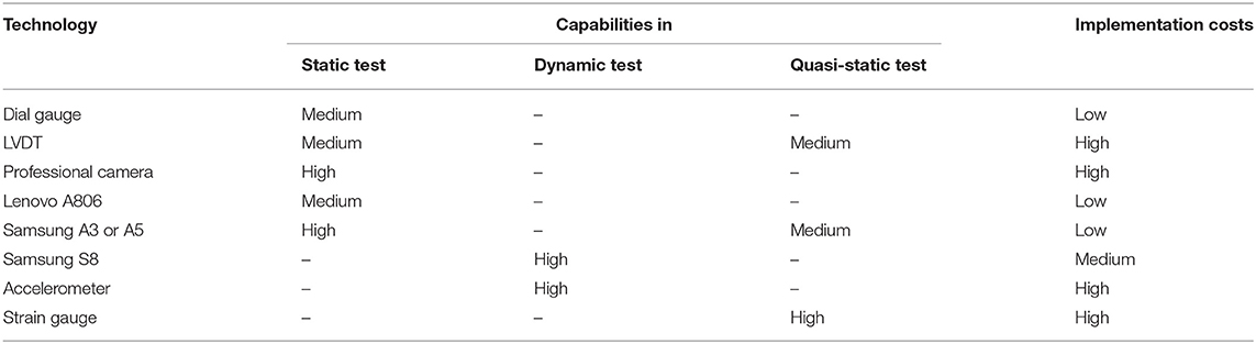
Table 3. Summary of the capability (high, medium, low) of the technologies used in the laboratory environment and their estimated implementation costs.

Conclusions

This study proposes a low cost vision-based system using smartphones for monitoring deformations in the laboratory environment, and compares structural response of laboratory structures against contact sensors and expensive image-based systems that make use of professional cameras and proprietary software. Very good agreements with structural response obtained from contact and vision-based systems are obtained for the static and dynamic tests. The quasi-static test brings more challenges that need to be addressed in the future studies. The following conclusions are drawn from the study:

• For the static test similar measurement accuracies are achieved from a professional camera and smartphones when analyzing images with both free image processing tools and proprietary software.

• The dynamic test presents that the high-grade Samsung S8 smartphone offers very similar results compared to standard contact sensors for a fraction of the cost of traditional sensors. In comparison to accelerometers, values obtained from the vision sensor repeatedly correlated with movement pattern and magnitude. Significant advantages of the vision sensor over traditional sensors include, but are not limited to, the contactless nature of measurement, no requirement for a power supply on site and cost.

• Low cost vision-based systems deploying smartphones for deformation monitoring have potential applications in laboratory environments. These systems could reduce costs of data acquisition systems and labor. The performance of such a proposed system has to be calibrated and compared with professional cameras and proprietary sensing systems (both contact and non-contact). It is anticipated that in near future smartphones will become faster and more powerful in their vision-based capacities than they are currently. Smartphones will allow taking high quality photos at high frequencies, therefore broadening their applications for measurement collection of full-scale structures.

• The consistency and repeatability of the results obtained from low-cost vision sensor/displacement calculation algorithms in a diverse variety of laboratory trials provide confidence in their usage. Further development of this system would involve a series of field trials to determine the accuracy of the systems in an uncontrolled environment and maybe even in long-term applications.

The results show that smartphone vision systems can provide accurate estimations of structural deformations at a fraction of the cost of using professional top of the range cameras. It is anticipated that with upcoming developments in smartphone technologies, smartphone applications are expected to become widely used in both the educational environment and for engineering applications.

Author Contributions

RK supervised the research, carried out experimental work, drafted the manuscript, contributed to image processing and writing. YX and DL contributed to the processing and writing. AA and JM contributed to writing.

Conflict of Interest Statement

The authors declare that the research was conducted in the absence of any commercial or financial relationships that could be construed as a potential conflict of interest.

Acknowledgments

The authors would like to thank Julius Ayodeji and Matthew Garlic who helped with experimental work.

References

Abdel-Jaber, H., and Glisic, B. (2016). Systematic method for the validation of long-term temperature measurements. Smart Mater. Struct. 25:125025. doi: 10.1088/0964-1726/25/12/125025

CrossRef Full Text | Google Scholar

Adhikari, R. S., Moselhi, O., and Bagchi, A. (2014). Image-based retrieval of concrete crack properties for bridge inspection. Autom. Constr. 39, 180–194. doi: 10.1016/j.autcon.2013.06.011

CrossRef Full Text | Google Scholar

Al-Habaibeh, A., and Parkin, R. M. (2003). Low-cost mechatronic systems for teaching condition monitoring. Int. J. Eng. Educ. 19, 615–622. Available online at: https://www.ijee.ie/articles/Vol19-4/IJEE1379.pdf

Google Scholar

Bay, H., Tuytelaars, T., and Van Gool, V. (2008). SURF: speeded - up robust features. Eur. Conf. Comput. Vis. 110, 346–359. doi: 10.1016/j.cviu.2007.09.014

CrossRef Full Text | Google Scholar

Brownjohn, J. M. W., Xu, Y., and Hester, D. (2017). Vision-based bridge deformation monitoring. Front. Built Environ. 3:23. doi: 10.3389/fbuil.2017.00023

CrossRef Full Text | Google Scholar

Choi, H.-S., Cheung, J.-H., Kim, S.-H., and Ahn, J.-H. (2011). Structural dynamic displacement vision system using digital image processing. NDT E. Int. 44, 597–608. doi: 10.1016/j.ndteint.2011.06.003

CrossRef Full Text | Google Scholar

Colwell, R. (1983). Manual of remote sensing. Am. Soc. Photogramm. 1, 1983–2440.

Google Scholar

Del Rincon, J. M., Hester, D., Lydon, D., Taylor, S., Brownjohn, J., and Lydon, M. (2018). Development and field testing of a vision-based displacement system using a low cost wireless action camera. Mech. Syst. Signal Process. 121, 343–358. doi: 10.1016/j.ymssp.2018.11.015

CrossRef Full Text | Google Scholar

Farrar, C. R., Duffy, T. A., Cornwell, P. J., and Doebling, S. W. (1999). “Excitation methods for bridge structures,” in Energy No. LA-UR-, NM (US).

Google Scholar

Feng, D., and Feng, M. Q. (2017). Experimental validation of cost-effective vision-based structural health monitoring. Mech. Syst. Signal Process. 88, 199–211. doi: 10.1016/j.ymssp.2016.11.021

CrossRef Full Text | Google Scholar

Girolami, A., Brunelli, D., and Benini, L. (2017). “Low-cost and distributed health monitoring system for critical buildings,” in Proceedings 2017 IEEE Workshop on Environmental, Energy, and Structural Monitoring Systems, EESMS 2017.

Google Scholar

Hameed, Z., Hong, Y. S., Cho, Y. M., Ahn, S. H., and Song, C. K. (2009). Condition monitoring and fault detection of wind turbines and related algorithms: a review. Renew. Sustain. Energy Rev. 13, 1–39. doi: 10.1016/j.rser.2007.05.008

CrossRef Full Text | Google Scholar

Hartley, R. I., and Mundy, J. L. (1993). “Relationship between photogrammmetry and computer vision,” in Integrating Photogrammetric Techniques With Scene Analysis and Machine Vision, Vol. 1944, (International Society for Optics and Photonics), 92–106.

Google Scholar

Hester, D., Brownjohn, J., Bocian, M., and Xu, Y. (2017). Low cost bridge load test: calculating bridge displacement from acceleration for load assessment calculations. Eng. Struct. 143, 358–374. doi: 10.1016/j.engstruct.2017.04.021

CrossRef Full Text | Google Scholar

Ho, H. N., Lee, J. H., Park, Y. S., and Lee, J. J. (2012). A synchronized multipoint vision-based system for displacement measurement of civil infrastructures. Sci. World J. 2012:519146. doi: 10.1100/2012/519146

PubMed Abstract | CrossRef Full Text | Google Scholar

Jiang, R., Jáuregui, D. V., and White, K. R. (2008). Close-range photogrammetry applications in bridge measurement: literature review. Meas. J. Int. Meas. Confed. 41, 823–834. doi: 10.1016/j.measurement.2007.12.005

CrossRef Full Text | Google Scholar

Khuc, T., and Catbas, F. N. (2017). Computer vision-based displacement and vibration monitoring without using physical target on structures. Struct. Infrastruct. Eng. 13, 505–516. doi: 10.1080/15732479.2016.1164729

CrossRef Full Text | Google Scholar

Kromanis, R., and Al-Habaibeh, A. (2017). “Low cost vision-based systems using smartphones for measuring deformation in structures for condition monitoring and asset management,” in The 8th International Conference on Structural Health Monitoring of Intelligent Infrastructure. (Brisbane, QLD).

Google Scholar

Kromanis, R., and Kripakaran, P. (2017). Data-driven approaches for measurement interpretation: analysing integrated thermal and vehicular response in bridge structural health monitoring. Adv. Eng. Informatics 34, 46–59. doi: 10.1016/j.aei.2017.09.002

CrossRef Full Text | Google Scholar

Kromanis, R., and Liang, H. (2018). “Condition assessment of structures using smartphones : a position independent multi-epoch imaging approach,” in 9th European Workshop on Structural Health Monitoring, July 10-13, 2018 (Manchester, UK), 1–10.

Google Scholar

Lowe, D. G. (1999). Object recognition from local scale-invariant features. Proc. Seventh IEEE Int. Conf. Comput. Vis. 2, 1150–1157. doi: 10.1109/ICCV.1999.790410

CrossRef Full Text | Google Scholar

Macdonald, J. H. G., Dagless, E. L., Thomas, B. T., and Taylor, C. A. (1997). Dynamic measurements of the second severn crossing. Proc. Inst. Civ. Eng. Transp. 123, 241–248. doi: 10.1680/itran.1997.29978

CrossRef Full Text | Google Scholar

McGetrick, P. J., Hester, D., and Taylor, S. E. (2017). Implementation of a drive-by monitoring system for transport infrastructure utilising smartphone technology and GNSS. J. Civ. Struct. Heal. Monit. 7, 175–189. doi: 10.1007/s13349-017-0218-7

CrossRef Full Text | Google Scholar

Min, J. H., Gelo, N. J., and Jo, H. (2015). Non-contact and real-time dynamic displacement monitoring using smartphone technologies. J. Life Cycle Reliab. Safety Eng. 4, 40–51. Available online at: https://www.researchgate.net/profile/Hongki_Jo/publication/286256215_Non-contact_and_Real-time_Dynamic_Displacement_Monitoring_using_Smartphone_Technologies/links/5667398c08ae34c89a02380b/Non-contact-and-Real-time-Dynamic-Displacement-Monitoring-using-Smartphone-Technologies.pdf

Google Scholar

Nayeem, I., and Want, R. (2014). Smartphones: past, present, and future. IEEE Pervasive Comput. 13, 89–92. doi: 10.1109/MPRV.2014.74

CrossRef Full Text | Google Scholar

Potter, K. D., Setchell, C., and Imetrum Ltd., (2014). Positional Measurement of a Feature within an Image. U.S. Patent 8,718,403.

Shakmak, B., and Al-Habaibeh, A. (2015). “Detection of water leakage in buried pipes using infrared technology; a comparative study of using high and low resolution infrared cameras for evaluating distant remote detection,” in Applied Electrical Engineering and Computing Technologies (AEECT). IEEE Jordan Conference on 2015 November 3.

Google Scholar

Stephen, G. A., Brownjohn, J. M. W., and Taylor, C. A. (1993). Measurements of static and dynamic displacement from visual monitoring of the humber bridge. Eng. Struct. 15, 197–208. doi: 10.1016/0141-0296(93)90054-8

CrossRef Full Text | Google Scholar

Tomasi, C., and Kanade, T. (1991). Detection and tracking of point features. Image 91, 1–22.

Google Scholar

Torr, P. H. S., and Zisserman, A. (2000). MLESAC: a new robust estimator with application to estimating image geometry. Comput. Vis. Image Underst. 78, 138–156. doi: 10.1006/cviu.1999.0832

CrossRef Full Text | Google Scholar

Xu, Y., and Brownjohn, J. M. W. (2017). Review of machine-vision based methodologies for displacement measurement in civil structures. J. Civ. Struct. Heal. Monit. 8, 91–110. doi: 10.1007/s13349-017-0261-4

CrossRef Full Text | Google Scholar

Xu, Y., Brownjohn, J. M. W., Hester, D., and Koo, K. Y. (2017). Long-span bridges: enhanced data fusion of GPS displacement and deck accelerations. Eng. Struct. 147, 639–651. doi: 10.1016/j.engstruct.2017.06.018

CrossRef Full Text | Google Scholar

Ye, X. W., Ni, Y. Q., Wai, T. T., Wong, K. Y., Zhang, X. M., and Xu, F. (2013). A vision-based system for dynamic displacement measurement of long-span bridges: algorithm and verification. Smart Struct. Syst. 12, 363–379. doi: 10.12989/sss.2013.12.3_4.363

CrossRef Full Text | Google Scholar

Yu, J., Meng, X., Shao, X., Yan, B., and Yang, L. (2014). Identification of dynamic displacements and modal frequencies of a medium-span suspension bridge using multimode GNSS processing. Eng. Struct. 81, 432–443. doi: 10.1016/j.engstruct.2014.10.010

CrossRef Full Text | Google Scholar

Yu, Y., Han, R., Zhao, X., Mao, X., Hu, W., Jiao, D., et al. (2015). Initial validation of mobile-structural health monitoring method using smartphones. Int. J. Distrib. Sens. Netw. 11:274391. doi: 10.1155/2015/274391

CrossRef Full Text | Google Scholar

Zhao, X., Liu, H., Yu, Y., Zhu, Q., Hu, W., Li, M., and Ou, J. (2015). “Convenient displacement monitoring technique using smartphone,” in Proceedings of the International Conference on Vibroengineering (Nanjing), 26–28. Available online at: https://www.researchgate.net/profile/Xuefeng_Zhao3/publication/296637401_Convenient_displacement_monitoring_technique_using_smartphone/links/56d93bc008aee1aa5f80464d.pdf

Google Scholar