Evaluation of XIMIS for Assessing Extreme Pressure Coefficients

Introduction

The design of buildings and their components to resist extreme winds requires the assessment of peak surface pressures. The use of scale models in wind tunnels for this purpose has been an active research topic since the early 1980s. Most published studies introduce and demonstrate methods and there have been only a few studies which compare and calibrate alternative methods [e.g., (Cook, 1982b), (Cook, 2016b)]. Cook (2016b) proposed to adapt the Harris (2009) penultimate XIMIS method, originally proposed for extreme wind speeds, for peak pressures, calibrating it against conventional Gumbel epochal extreme value analysis (EVA) and the recent Gaussian process model using moment-based Hermite polynomials, here denoted as the “moment-based Hermite polynomial translation model” (HPM) by Yang et al. (2013) (YGP) using very long records of wind tunnel data. Since Cook (2016b) was a discussion paper for Huang et al. (2016) which promotes the use of HPM for non-Gaussian process data, only a brief explanation of XIMIS as well as the comparison results using only 2 pressure taps on a roof of low-rise building were presented. As mentioned in the conclusions of Cook (2016b), a calibration using only two taps is not sufficient to present the accuracy and benefit of XIMIS. Hence, this study provides the extensive explanation of the XIMIS method and a comprehensive calibration of XIMIS against EVA and HPM using data from 496 roof taps to quantify the value-dependence and separation/attachment zonal dependence.

The data supporting this demonstration are from a series of tests at the University of Western Ontario (UWO), Canada, to provide comparison data for the Florida Coastal Monitoring Program (Balderrama et al., 2011). Figure 1 shows the model, the location of 496 pressure taps distributed over the roof and the wind direction tested. Four taps are marked for later reference: Tap A corresponds to the highest recorded peak suction (−12.9 for Cp referenced to mean roof height) and lies in a permanently separated-flow region behind the ridge in the gable corner; Tap B corresponds to a generally attached flow region with transient separations; Tap C corresponds to the highest recorded kurtosis (21.04); and Tap D corresponds to the maximum positive mean pressure coefficient (2.62). The pressure coefficient data had been sampled at 40 Hz for 30 h, equivalent full scale (FS), assuming a time scale of 1/100, giving 4,320,000 values for each tap. Figure 2 shows the first 10 min (FS) of Cp at tap A as an example of the highly-skewed non-Gaussian character of the Cp in a separated flow zone. The detail of the wind tunnel tests can be found in Kopp and Gavanski (2010). In all the following analyses, only the peak suction Cp values have been used.

FIGURE 1

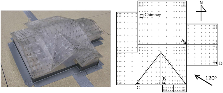
Figure 1. Model, tap layout and wind direction (wind direction of 0 deg is from the north direction).

FIGURE 2

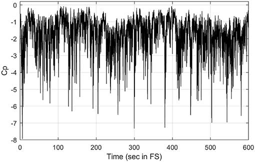
Figure 2. Example Cp time series for Tap A.

Previous Peak Estimation Methods

Various methods of peak estimation have been suggested to characterize local peak pressure coefficients based on observed peaks: from a single extreme value recorded during a sampling period (e.g., Stathopoulos, 1979), the mean of several observed peaks (e.g., Holmes et al., 1989), to the value at a chosen fractile of a probability distribution fitted to the observed peaks. In terms of the last method, the most common method fits the Fisher-Tippett Type I (FT1) distribution to the peak value in a number of epochs (e.g., Cook and Mayne, 1979, 1980). This is known as a Gumbel epochal extreme value analysis (EVA). When curvature is observed in the upper tail, from incomplete convergence (Cook et al., 2003; Cook and Harris, 2004), the Fisher-Tippett Type III (FT3 or Reverse Weibull) distribution, which can mimic this curvature by its additional parameter, has also been adopted (Holmes and Cochran, 2003; Kasperski, 2003). It is noted that there are number of studies which doubt the validity of the FT3 distribution for this purpose (e.g., Harris, 2006).

As all the epochal methods use only the largest maxima in each epoch and ignore the 2nd, 3rd, etc. largest maxima, it is likely that better estimation is possible with more efficient use of the data. With this reasoning, the Peaks-Over-Threshold (POT) method was suggested (Simiu and Heckert, 1996; Holmes and Moriarty, 1999) and uses all the data above a certain high threshold. One example of its use is to ensure statistical independence of wind speed data from mixed climates by limiting the data to the upper tails (Cook et al., 2003). A common form of the POT method fits to the Generalized Pareto distribution (GPD), the appropriate distribution for the exceedances of a high threshold when convergence has been achieved to one of the extreme value distributions. It is noted that the use of GPD with POT data requires a high threshold and a large population, typically more than 100,000 peaks for a good convergence at the upper bound (Galambos and Macri, 1999), which seems to be unrealistic amount of data to obtain. This is because GPD is an asymptotic distribution of the generalized extreme value distribution (GEV) (Holmes and Moriarty, 1999), which is also asymptotic to extreme-value distributions for a parent variable, so it is doubly difficult to achieve convergence.

Since both FT1 fitting and POT methods assume asymptotic distributions, and this is difficult to verify using the typical data lengths, the average conditional exceedance rate method (ACER method) was proposed (Karpa and Naess, 2013). This method has benefits over the other existing methods such as it does not require convergence, statistical independence or stationarity. The ACER method constructs a cascade of conditional probability distributions having the target distribution function of the extreme value as the limit. This is calculated by the estimation of the average conditional exceedance rates. It is like the POT method except that it counts downwards from the extreme instead of upwards from the threshold.

Finally, there is the classical Davenport Peak Factor Method (DPFM). This estimates the expected peak, X_peak, whose duration is T, in terms of the peak factor, g, defined as:

$\begin{array}{ll}g=\left\{E\left[X_{peak\text{\_}T}\right]-m_X\right\}/{\sigma }_X& (1)\end{array}$

where m_X and σ_X are the mean and standard deviation of X, respectively. With the assumption that X follows the Gaussian distribution, the distribution of X_peak converges onto the FT1 distribution. Davenport (1964) suggested the expression of peak factor defined in Equation (2)

$\begin{array}{ll}g=\sqrt{2ln(\nu T)}+\gamma /\sqrt{2ln(\nu T)}& (2)\end{array}$

where ν is the mean up-crossing rate across zero and γ is Euler's constant of 0.5772.

It is well-known that, Equation (2) works well for a Gaussian process but not for non-Gaussian processes, such as the wind pressures in flow separation regions. Since peak factors of “softening” non-Gaussian processes (kurtosis > 3) are larger than that of a Gaussian process, Equation (2) is not appropriate. To obtain the peak factor for softening non-Gaussian processes, Kareem and Zhao (1994) first suggested correcting the moment-based Hermite polynomial translation model (HPM). A slightly different formulation was presented in Chen and Huang (2009). Kwon and Kareem (2011) revised HPM to overcome conservatism when the process is strongly non-Gaussian, but the HPM parameters become less accurate as wind pressure coefficient deviates strongly from Gaussian. To deal with this limitation, Yang et al. (2013) suggested an alternative closed form approximate relationship between the skewness and kurtosis of the HPM shape parameters. Peng et al. (2014) further suggested a mixed distribution model to capture both the tail and bulk probability regions of the marginal distribution, where an empirical distribution from the measured data and GPD are applied in the bulk and tail probability regions, respectively. Instead of using the approximate solution for the HPM parameters, Huang et al. (2016) suggested to solve the non-linear equation via Newton-Raphson iteration. Liu et al. (2017) pointed out the fact that the traditional definition of skewness and kurtosis are affected by both distribution tails. This results in less accuracy of the translation model based on these two moments, for specifying only one of the distribution tails, and suggested a new moment-based HMP approach.

For “hardening” non-Gaussian processes (kurtosis <3), Ding and Chen (2014) extended the moment-based Hermite polynomial translation model with empirical formulations for determining the translation model coefficients. Reflecting the necessity of the determination of the extreme values of the combination of multiple variables in structural designs, Folgueras et al. (2016) suggested extended Davenport peak factor, which can estimate the extreme values of the resultant of the linear combination of multiple Gaussian and non-Gaussian random variables that come from a common agent. Ma and Xu (2017) suggested new peak factor calculation method by employing Johnson transformation to fit the marginal distribution of the non-Gaussian process and estimating extrema on long-tail and short-tail sides separately.

Other methods for estimating non-Gaussian processes have also been suggested. Sadek and Simiu (2002) identified the appropriate marginal probability distribution for the non-Gaussian time series using the probability plot correlation coefficient (PPCC) method. The three-parameter gamma distribution and normal distribution were selected as the best model for the longer and the shorter tails of the marginal distribution, respectively. Then, the distribution of the peaks of the non-Gaussian variate is estimated by using the standard translation process approach. Tieleman et al. (2007) employed Sadek and Simiu's method but with more wind tunnel data. It shows that instead of PPCC method to calculate the parameters of gamma distribution, the method of moments can be used with acceptable precision but with much less computational time. Huang et al. (2013) modified the translation procedure proposed by Sadek and Simiu (2002) such that cumulative distribution function (CDF) of the non-Gaussian process was estimated using the kernel-smoothing method instead of assuming a gamma distribution. In addition, the peaks of the Gaussian process are first generated from a Rayleigh distribution instead of the Rice's formula [Equation (2) in Sadek and Simiu (2002)], and the mapped peak data of the standardized non-Gaussian process are fitted to the Weibull distribution, instead of Gumbel distribution. This was named the translated-peak-process method (TPP method). Huang et al. (2013) also suggested a closed-form expression of Weibull peak factor based on extreme value theory, which can be calculated using the Weibull parameters obtained from the TPP method. Ding and Chen (2014) emphasized an accurate modeling of the upper tail behavior of the translation function and suggested the CDF-based translation method with the use of GPD to model the distribution tail over a given threshold.

As reviewed above, the use of non-Gaussian peak factor obtained by translation method has recently been an active research topic as a method of peak wind pressure coefficient estimation. In the meanwhile, XIMIS, a method which has worked very well for analyzing extreme wind speeds using independent storm or m-day maxima was adapted to extreme pressure coefficients (Cook, 2016b). The benefit of XIMIS over all the existing peak estimation methods are:

1. Since it is penultimate, not asymptotic, the assumption of rT → ∞, where r is rate of occurrence and T is epoch for extreme, which is difficult to satisfy in practice, is not required;

2. This method can be applied to any independent peak data, including epoch maxima, but also including heavily left-censored, POT data;

3. The total population of independent peaks is not required as prerequisite, provided it is large (more than 30).

XIMIS

Development of XIMIS From EVA

EVA has been a standard method to estimate peak wind speed and wind pressure coefficients since 1970s, and was the starting point of pursuing better methods, culminating in XIMIS.

Peterka and Cermak (1975) were the first to show that the form of the probability density function (PDF) of surface pressures varies from nearly Gaussian in attached flow regions to exponential in the tails in separated regions. Recently a Gaussian-Exponential mixture model was proposed to address the range of PDFs found in practice (Cook, 2016a). All these PDFs are members of the exponential class of distributions:

$\begin{array}{ll}F(x)=1-exp\left\{-h(x)\right\}& (3)\end{array}$

where h(x) → ∞ as x → ∞. From extreme value theory, the appropriate asymptotic form when the parent distribution is of the exponential class is the Fisher-Tippett (FT1) distribution.

$\begin{array}{ll}\Phi (x)=exp\left[-exp(-y)\right]=exp\left[-exp\left\{-a(x-U)\right\}\right]& (4)\end{array}$

where x is extreme variate, y is the standard reduced variate and a and U are the dispersion and location parameters, respectively.

The conventional Gumbel extreme value analysis of annual maximum wind speed takes the following steps:

1. The largest wind speed is extracted from each year of the record and the values ranked in ascending order of magnitude, giving m = 1 to the smallest value through m = N to the largest.

2. Each wind speed is associated with a probability ordinate, P_m, derived from its rank with one of the following equations:

$\begin{array}{ll}{P}_m=\frac{m}{(N+1)}\text{Weibul}{\text{l}}^{\prime }\text{sestimator}& (\mathrm{5a})\end{array}$

(Gumbel, 1958)

$\begin{array}{ll}{P}_m=\frac{(m-0.44)}{(N+0.12)}\text{Gringorte}{\text{n}}^{\prime }\text{sestimator}& (\mathrm{5b})\end{array}$

(Gringorten, 1963)

where m = 1, 2, … N. The distinction between these two estimators is one of mean bias created by the non-linear form of Equation (4). Equation (5a) is an estimator for the mean probability, 〈P〉, and is the unbiased estimator for the probability of the m-th observed value. Equation (5b) is an estimator for the probability of the mean reduced variate, 〈y〉, and is the unbiased estimator for a value with a given probability. The two are not concomitant, as discussed more fully in Cook (2012), however the distinction only significantly affects the top few ranks when N is large.

3. With P_m obtained as above, the reduced variate, y, can be estimated by the following equation:

$\begin{array}{ll}y=-ln\left[-ln(P_m)\right]& (6)\end{array}$

4. Plotting the wind speed, V, against the corresponding estimate for y linearizes, Equation (4), so the FT1 distribution parameters, a and U can be obtained from its slope and intercept. The alternative is to use least square regression or the generalized least square method (such as Hong et al., 2013) or more sophisticated methods such as maximum likelihood.

An alternative, commonly used, method which gives unbiased estimates of a and U directly from the N ranked extremes is the “Best linear unbiased estimator” (BLUE) method of Lieblein (1974), but the necessary coefficients are only available for N ≤ 24, as values for larger N becomes increasingly unreliable (Hong et al., 2013).

The appropriateness of the FT1 asymptotic distribution depends on the convergence of the exact distribution, expressed as F(x)^N where x is a statistically independent parent. Convergence depends on the number of extremes, N, as well as the form of the upper tail of parent distribution.

For wind speeds, several methods have been proposed for augmenting the annual extremes to increase the sample size, N. Where continuous meteorological data are available, Cook (1982a) proposed identifying individual storms and extracting the maximum wind speed from each. This is the original Method of Independent Storms (MIS) which was eventually developed into XIMIS. Where only daily maxima or values above a certain threshold are available, Simiu and Heckert (1996) ensured independence, by selecting m-day maxima, where m longer than the typical storm duration. This gives a substantial increase of sample size over conventional EVA and a corresponding improvement in analysis accuracy. The same principles apply to peak surface pressures.

The general procedure of MIS uses r independent storm maxima per year instead of just one. The probability distribution of the largest annual maxima out of r independent maxima per year, becomes (P_m)^r and changes Equation (6) into

$\begin{array}{ll}y=-ln\left[-ln{(P_m)}^r\right]=-ln\left[-r(P_m)\right]& (7)\end{array}$

When only epoch maxima, or similar data are available, the conventional Gumbel extreme value analysis has been the usual method of choice. The standard graphical fitting method (Gumbel, 1958) assumes that the statistical variance of all points is uniform and gives each point the same weight. This is not true especially for the largest values; hence, the Lieblein BLUE method, which gives the more weight to the middle-ranked extremes, was employed for the determination of parameters in Cook (1982a) instead. However, the BLUE method uses of look-up table for N ≤ 24 and an approximate method for the higher N obtained using MIS. Harris (1996) suggested an improved set of plotting positions as well as the application of weighted least squares technique to fit a straight line for the estimation of a and U in Equation (4). This new method does not require the look-up of tabulated coefficients like the Lieblein BLUE and offers an improvement in accuracy over the BLUE and Gringorten methods.

Later, Harris (1999) adapted this method to apply to independent storm maxima, giving new plotting positions and fitting weights to reduce the systematic error caused by fitting (P_m)^r to the FT1 asymptote in MIS, calling this the “Improved Method of Independent Storm (IMIS).” Because these new plotting positions become less accurate in the lower tail, Harris suggested censoring the distribution below a threshold at the plotting position for the smallest annual maximum and demonstrated that the results are not sensitive to the exact threshold value.

Harris (2001) examined the accuracy of IMIS by comparing the estimated 50-yr return period wind speed with other methods. The selected methods were:

1. The conventional Gumbel extreme-value method (Method 1) fitted by classical least square;

2. Method 1 but using the Lieblein BLUE method to remove bias;

3. The method suggested by Harris (1996) with weighted least square, and;

4. IMIS as proposed by Harris, 1999.

Harris (2001) showed that IMIS has very small bias and the lowest variability among all methods considered and hence should be preferred when sufficiently continuous data are available.

In order to avoid the issue of asymptotic convergence (i.e., rT → ∞ where T is the reference epoch, e.g., T = 1 year for annual maxima), which is the necessary assumption to use the asymptotic FT1 model, Cook and Harris (2004) developed a general penultimate FT1 model, applicable as the penultimate distribution of extremes when the parent distribution has the Weibull form or right-tail equivalent to the Weibull form. This general penultimate FT1 distribution is expressed as:

$\begin{array}{ll}\text{Ψ}(x)=exp[-exp\left\{\frac{1}{c_T^k}(x_T^k-U_T^k)\right\}]& (8)\end{array}$

where x_T is the largest wind speed and U_T is characteristic largest value of wind speed in epoch T. c_T is the scale parameter and k is the shape parameter of the parent Weibull distribution.

Comparisons between this new method as well as the use of the ultimate asymptotic FT1 and general extreme value distributions (GEV) were performed using annual maxima and storm maxima wind speed data. The latter was derived by Cook (1982a), using the bootstrapping procedure derived by Cook (2004). It was proven that the use of general penultimate FT1 distribution can provide at least as good an empirical fit as the asymptotic GEV distribution. The penultimate FT1 has the additional benefit of being able to produce identical results regardless of whether it is wind speed or dynamic pressure. The GEV produces different results for wind speed and dynamic pressure which is indefensible as the basis of a design standard.

The XIMIS Method of Harris, 2009

In the final iteration of improvements, Harris (2009) introduced XIMIS, an extension of the existing IMIS method (Harris, 1999). It uses the general penultimate distribution of extremes. The benefit of this method is that this can be applied to different sets of mutually independent data drawn from the original parent to give the same exact distribution of maxima: including independent storm maxima, m-day maxima, and event (e.g., thunderstorm or cyclone) maxima. The other benefit is that this method does not require the total population of the data, N, to be known in advance, provided N is sufficiently large. This allows the method to be applied to heavily left-censored data. Compared with these advantages, the requirement of XIMIS is merely that the occurrence of the independent events is a Poisson process or that rT is large enough to validate the Cauchy formula for the exponential when an underlying Poisson process cannot be assumed. Harris (2009) validated the XIMIS method using wind speed data at three different locations.

The XIMIS unbiased mean reduced variate for the largest peak in an epoch, is:

$\begin{array}{ll}\overline{y_1}=ln(R)+\gamma =ln(R)+0.5772& (9)\end{array}$

where R is the number of datum epochs in the observation period and has a relationship of N = RrT; and, assuming the Poisson process model for independent events applies for the other ranks, m, by the generating function:

$\begin{array}{ll}\overline{y_{m+1}}=\overline{y_m}-\frac{1}{m}& (10)\end{array}$

where m is the rank in decreasing value from the largest. The principal advantage of these plotting positions is that the number of independent values, N in Equation (5), is not required. Hence, XIMIS is applicable heavily left-censored or peak-over-threshold data – a feature which is exploited in this study.

Equation (9) is the exact analytical expression for the largest rank of the FT1 distribution, and also for the exponential distribution to which the FT1 converges in the upper tail. The exponential class pressure coefficients converge extremely rapidly. The ln(R) term represents the Poisson shift in the other extreme value analysis methods. Equation (10) is the Gumbel (1958) generating function for the exponential distribution (Expression (8) on P116) but working down from the highest ranked value instead of up from the lowest. The accuracy of Equation (10) decreases in the lower tail as FT1 diverges from exponential and significant error must be eliminated by left-censoring. Harris (2009) gives ε_y = exp (–y)/(2N) as a first-order approximation to the error in the lower tail. This is shown in Figure 3, where the dashed line for the minimum observed N, which is 4,485 obtained from the currently employed dataset, indicates the difference remains less than ε = 0.01 down to y = −4.5. This is further into the lower tail than previous methods and increases the amount of data contributing to the analysis.

FIGURE 3

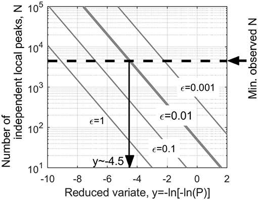
Figure 3. XIMIS model error in y for lower tail.

Figure 4 shows the XIMIS analysis for the 100 highest suction peaks in the Cp time series at Tap A, for T = 160 min FS, plotted on Gumbel axes. These suction peaks in Cp time series will be denoted as “local peaks,” in order to avoid confusion with the estimated peak “minima” by XIMIS or other estimating methods. The number of the estimated peak minima will be denoted as N_peak. The open circle symbols show the ranked estimated peak values from a single trial and the solid circles show the average for all 11 (~30 × 60/160 = N_peak) trials. The + markers above and below each value show ±1 standard deviation for the 11 trials—all the values shown here lie inside this range, however, obviously, this is not always the case for the other 10 trials. The left-hand tail, truncated at the 100th largest local peak, remains within the ε_y = 0.01 error boundary, indicating more local peaks could have been used. The effect of the number of local peaks employed for the estimation of peak will be discussed in section Applicability of XIMIS to Wind Pressure Coefficients. The FT1 fit for the single trial is shown by the solid line and the average of all 11 trials by the dashed line. These, and the fits for the other pressure taps, were made by unweighted least-mean-squares, using the standard slope and intercept functions in Matlab. Harris (2009) recommends weighting each value by the reciprocal of the rank variance, 1/σ ²(y), when fitting: where σ ²(y₁) = π²/6 = 1.645 … and σ ²(y_n+1) = σ ²(y_n)−1/n²; but this extra complication is necessary only with short data sets and makes virtually no difference with 100 values. The intercept corresponds to the FT1 mode, U, and the slope to the inverse of dispersion, 1/a, from which the 78% hourly-peak value is: Cp = U + 1.4/a.

FIGURE 4

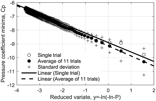
Figure 4. Gumbel plot from XIMIS method, T = 160 min, for Tap A.

Methodology

Each of the analysis methods described below was implemented twice, using the data for Taps A and B: once by NJC using Excel spreadsheets; and again, by EG using a MATLAB script. Discrepancies between the two implementations were investigated and any errors were corrected before the data from all the taps were processed by EG using MATLAB.

Applicability of XIMIS to Wind Pressure Coefficients

The XIMIS method requires that the peak values are independent and follow the Poisson recurrence model. In the preliminary calibration of Taps A and B (Cook, 2016b), the 100 highest local suction peaks were used assuming independence, as in Peterka (1983), and their independence was checked subsequently. Here a de-clustering algorithm was applied, equivalent to the “storm search” in Cook (1982a) but based on the up/down-crossings of the mean, i.e., the same as the assumption inherent in the Davenport peak factor method. The largest local peak suction was extracted between each down-crossing of the mean and the following up-crossing. Hence, the number of independent local peaks, N = rT, where r is the mean crossing rate (MCR) in the YGP method, will be obtained in the process of XIMIS method, but, as previously noted, the method does not use this value—it merely needs to be large.

The top 100 independent suction peaks used here correspond to just 0.5 to 2% of all independent local peaks in 30 h FS. This prompts the question: as this is a small proportion, is the additional overhead of de-clustering necessary? The number 100 was selected in the current analysis simply because it is a nice large round number. This choice was tested by examining how the COV (= standard deviation/average) of the estimated peak varies with this number of minima used, n₁, in Figure 5. As expected, the COV decreases as n₁ increases, n₁ = 100 corresponds to a COV of 0.1. However, the COV continues to decrease for larger n₁, indicating accuracy could be improved provided the ε_y criterion in Figure 3 is not exceeded.

FIGURE 5

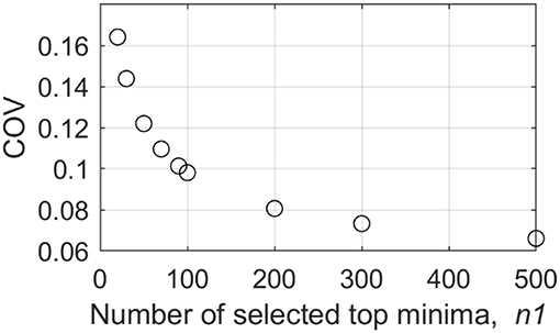
Figure 5. The variation of COV of estimated Cp peak with the number of top minima in XIMIS.

If the Cp peaks follow the Poisson recurrence model, as required by the XIMIS method, the inter-arrival times, τ, will be exponentially distributed (Brabson and Palutikof, 2000). This is tested by plotting the inter arrival time of selected local suction peaks on exponential axes in terms of the unbiased estimator for an exponential distribution, y = –ln(1–P) and checking whether the regression coefficient, R², becomes close to 1.

The calculated R² values for all 496 taps were plotted as contours over the roof in Figure 6 where white color indicates R²~1. These contours indicate the high linearity of τ and y for most of the taps and considered T. Based on these results, it is concluded that a Poisson process model can be applicable for Cps; hence, XIMIS is valid for wind pressure coefficients.

FIGURE 6

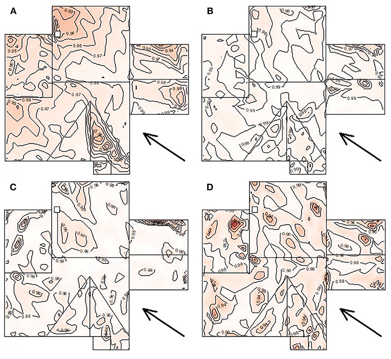
Figure 6. Contour of the regression coefficients, R², of the inter arrival time of selected local suction peaks, τ, for different epochs: (A) 60 trials of T = 30 min, (B) 11 trials of T = 160 min, (C) 3 trials of T = 10 h, (D) 1 trial of T = 30 h.

Consistent Basis for Comparison

As the basis adopted for comparison in order to present the performance of XIMIS, the 78% fractile of the fitted Fisher-Tippett Type 1(FT1) distribution of hourly-peak suction values was selected. This is the standard method employed for peak estimation in UK and is frequently employed by wind researchers/engineers, worldwide, for its simplicity (Gavanski et al., 2016). This fractile corresponds to the reduced variate y = 1.4 for T = 1 h FS epochs and stems from the simplified Cook-Mayne method (Cook and Mayne, 1980) which accounts for the joint statistics of wind speed and pressure coefficient, and has become a de-facto international standard. Many of the other cited works also use this datum.

Because the methods described below use a range of actual or implied epochs, T, it is necessary to adjust the results to a datum period, T = 1 h, for a consistent comparison. For EVA, a characteristic of the FT1 distribution is that results from one epoch, T₁, may be translated to another epoch, T₂, by applying the “Poisson shift,” Δy = ln(T₁/T₂) so, for example, that 10 min peaks are translated to 1 h peaks using Δy = –ln(60/10), as demonstrated in the previous calibration exercise of Cook (1982b). For the YGP method, the mean crossing rate, r, is expressed as crossings per hour. For XIMIS, this is by adjusting R in Equation (9). For example, for the one hundred and eighty 10-min records, R = 10/60 = 1/6 because the record is shorter than the datum epoch, but for the whole 30 h record, R = (30*60)/60 = 30 because the record is larger than the datum epoch.

Datum Extreme-Value Analysis

The extremely long data record allows the standard EVA to estimate the 78% fractile to an unprecedented degree of accuracy, as a datum to assess the other methods. For the datum EVA, the Cp record was divided into 180 epochs of T = 10 min FS and the peak local suction Cp extracted from each. Figure 7A shows the Gumbel plots for the four marked taps using the Gringorten (1963) unbiased plotting positions of Equation (5b), together with the fitted FT1 models (straight lines) and the 5%/95% bootstrapped confidence limits (dashed curves). The data are an excellent fit to the model in the body of the distribution and the tails remain within the confidence limits. As there is no discernible curvature in these plots, there is no justification for fitting a GEV model, since its shape parameter will not be distinguishable from zero. Figure 7B shows the distribution of the datum 78% values over the roof after applying the Poisson shift to T = 1 h FS.

FIGURE 7

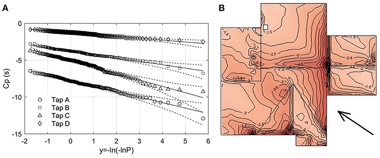
Figure 7. Datum extreme-value analysis: (A) Gumbel plot for Taps A to D, T = 10 min FS, (B) Distribution of 78% Cp, T = 1 h FS.

“Industry Standard” Extreme-Value Analysis

For comparison with historical industry practice, the data were subdivided into sets of N = 16 epochs of T = 10 min FS, giving 11 independent trials of 160 min records (N_peak = 11), each of which were assessed in exactly the same manner as the datum EVA.

The Hermite-Davenport Method of Yang et al. (2013)

From the extensive review of Cp peak estimation methods in section Previous Peak Estimation Methods, it is clear the non-Gaussian peak factor obtained by moment-based Hermite polynomial translation model has received the attention of many researchers. Among several studies dealing with this model, the method suggested by Yang et al. (2013), which will be denoted as “YGP method” hereafter, will be selected for our calibration of XIMIS method because of its relatively simple use and accuracy examined by several researchers (Peng et al., 2014; Liu et al., 2017; Ma and Xu, 2017; Song et al., 2019).

The YGP method was implemented for 30 trials of T = 1 h FS, and the first four moments were computed for each. The Davenport's peak factor was evaluated from the datum fractile P = 0.78 and the MCR by directly counting down-crossings of the mean, giving hourly rates in the range 4,400 < r < 20,000. The Hermite shape parameters, c₃ and c₄ in YGP were evaluated from the YGP polynomial expressions, enabling the Hermite transformation and the 78% fractile Cp to be computed. The YGP polynomial expressions evade the need to apply the Choi & Sweetman test (Yang et al., 2013) to see whether the transformation is valid, but only 17 of the 496 taps fail this test, including Tap A.

The evaluation steps for the following three methods are listed in Table 1 to show XIMIS is not difficult to implement compared with the other methods.

TABLE 1

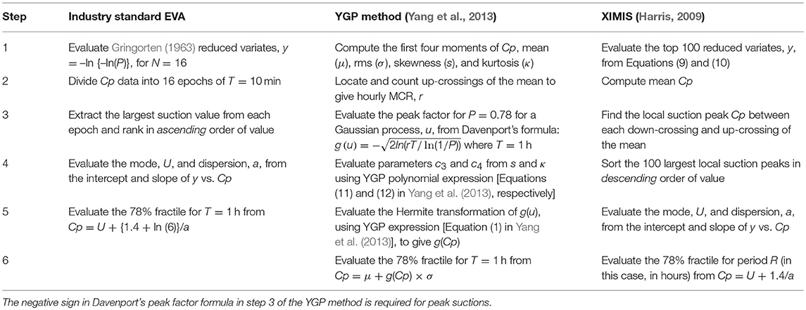
Table 1. Evaluation steps for the three methods.

Results

Method Bias Ratio

The bias ratio (method value/datum value) averaged over all taps is commonly used as a simple basis of comparison between methods. With multiple trials, the overall performance of a method may be expressed as the average bias for all trials and the statistical variability by the standard deviation between trials. Figure 8 displays the overall performance of the methods as ranges with the average in the center of each range, and plus/minus one standard error either side. The average is calculated as the average of estimated peaks for each tap calculated by the method divided by the average of the datum peaks. The standard error is calculated as square root of the average squared standard deviation for each tap, divided by the average of datum peak. It is immediately apparent, from the way the ranges for each method overlap, that the natural statistical variation dominates over the differences between methods. All XIMIS methods except T = 30 h FS underestimate compared with the datum although the amount, as well as the variation, becomes less for larger T. For XIMIS method of T = 160 min FS, which requires the same length of Cp time series as the industry standard EVA method (EVA N = 16 and T = 10 min), statistical variability is apparently less than the industry standard EVA, which indicates the superiority of XIMIS (Note: For XIMIS at T = 30 h, the standard error of the single trial was estimated by extrapolating the trend from the other cases). However, the YGP method significantly underestimates. The YGP results for other values of T, not reported here, are virtually identical.

FIGURE 8

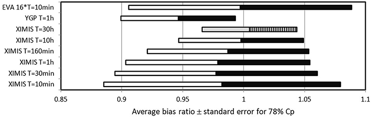
Figure 8. Average of performance of methods.

Figure 9 presents the average bias ratio for each tap calculated by different methods where white color indicate bias ratio ~1 and warm and cold colors indicate deviation from 1 (below 1 and above 1, respectively). Again, the superior performance of XIMIS is clear for all epochs considered over YGP.

FIGURE 9

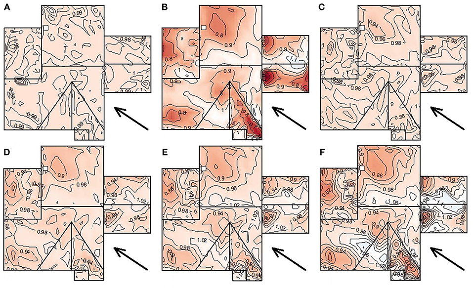
Figure 9. Spatial distribution of the average performance for each method: (A) EVA N = 16 and T = 10 min (N_peak = 11), (B) YGP T = 60 min (N_peak = 30), (C) XIMIS T = 160 min (N_peak = 11), (D) XIMIS T = 60 min (N_peak = 30), (E) XIMIS T = 30 min (N_peak = 60), (F) XIMIS T = 10 min (N_peak = 180).

The issue with the average bias ratio is that it gives every tap the same influence, or weight, irrespective of its value. As the highest suctions are confined to the taps close to the windward edges of each roof slope, the average is biased toward the many more taps where the suctions are much lower. Figure 10A displays the bias ratio for each individual tap, averaged over the 30 trials for T = 1 h, for the XIMIS methods plotted against the datum values. Although the scatter is greater at the lower suctions, XIMIS shows close to unity at higher suctions.

FIGURE 10

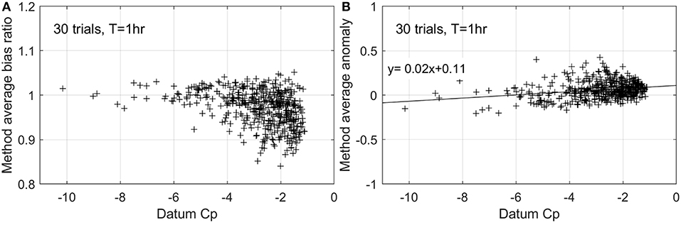
Figure 10. XIMIS bias and average anomaly vs. datum design value for T = 1 h records (N_peak = 30): (A) bias (method/datum), (B) anomaly (method—datum).

Method Anomaly

The anomaly (method value—datum value) may be a better measure of performance, especially for assessing cladding, because it is a direct measure of how wrong a value can be—as these are suctions, negative anomaly indicates conservatism and positive anomaly indicates non-conservatism. Figure 10B presents the average anomaly for each tap for the same cases as in Figure 10A and shows that the regression line for the XIMIS anomaly remains close to zero.

A key question is whether these anomalies are random or caused by the physics of the flow over the roof. Figure 11 shows the average anomaly for all trials of the methods plotted as contours over the roof where white color indicates anomaly ~ 0 and warm and cold colors indicate deviation from 0 in the negative and in the positive, respectively, using consistent contour intervals and shading for direct comparison:

(a) The EVA, using 16 epochs of T = 10 min, shows the least anomalies, within ±0.05 across most of the roof, and is a vindication of the “industry standard.”

(b) The YGP method for T = 1 h shows the most anomalies, ranging from overestimation by −0.5 in the zones of high suction to underestimation by more than +1 over much of the rest of the roof. The distinct patterns of anomalies over the roof indicate they are caused by the physics of the flow. Other values of T showed virtually the same anomalies, so are not shown.

(c) to (f) The XMIS method for values of T from T = 160 min down to T = 10 min shows the same patterns of anomalies emerging but with the increase of overestimation for suction peaks as the value of T decreases. At T = 160 min, (c) is directly comparable with (a) but, surprisingly, shows slightly higher anomalies. Previous experience suggests XIMIS should perform better because it exploits more data (Perhaps it does, and it is because it exploits more data that it is better able to reveal the physical patterns). The key finding is that using the shortest feasible record length, T = 10 min, the XIMIS method still performs significantly better than the YGP method.

FIGURE 11

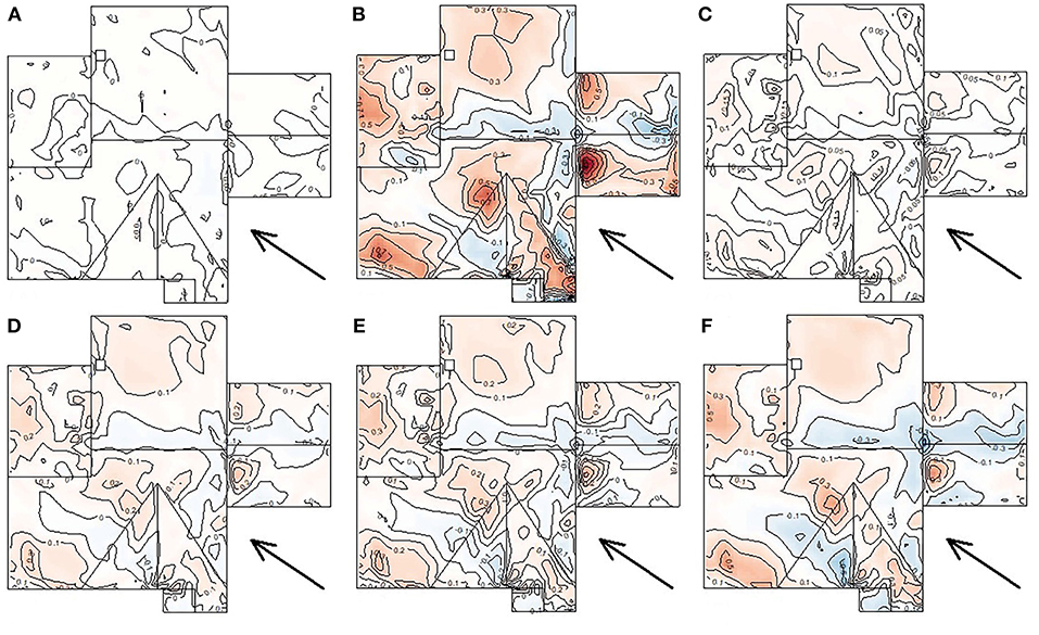
Figure 11. Spatial distribution of the average anomaly for each method: (A) EVA N = 16 and T = 10 min (N_peak = 11), (B) YGP T = 60 min (N_peak = 30), (C) XIMIS T = 160 min (N_peak = 11), (D) XIMIS T = 60 min (N_peak = 30), (E) XIMIS T = 30 min (N_peak = 60), (F) XIMIS T = 10 min (N_peak = 180).

Quantile-Quantile Plots

The quantile-quantile (Q-Q) plot is another common approach for assessing performance. Figures 12A,B show the N = 16 and T = 10 min EVA and T = 160 min XIMIS averaged values for each tap plotted against the datum 78% Cp, respectively. The positions of the four taps A to D are shown. Two regression lines were fitted: one a conventional fit, giving slope and intercept; and the other a fit forced through the origin, giving only a slope. The fit forced through zero has a slope marginally to the underestimate side of unity, while the conventional fit has a slope marginally to the overestimate side of unity and an intercept to underestimate side of zero—echoing the results in sections Method Bias Ratio and Method Anomaly, respectively. In all cases, the regression coefficient R² > 0.998 would generally be taken to indicate an excellent fit and the differences between these two methods to be insignificant.

FIGURE 12

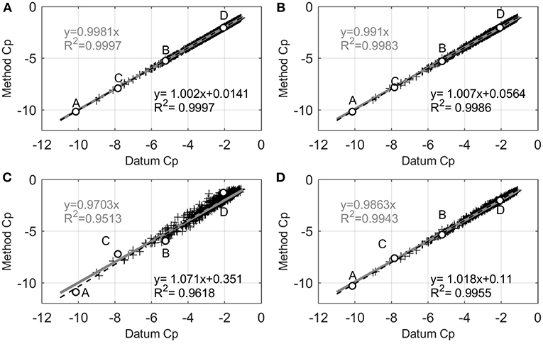
Figure 12. Q-Q plot for each method: (A) EVA N = 16 and T = 10 min (N_peak = 11), (B) XIMIS T = 160 min (N_peak = 11), (C) YGP T = 60 min (N_peak = 30), (D) XIMIS T = 60 min (N_peak = 30).

Figures 12C,D show similar Q-Q plots of the YGP method and XIMIS for T = 1 h, respectively. There is significantly more scatter in the YGP method than in XIMIS and this is reflected in the lower regression coefficients. The two slopes for the YGP method diverge from unity by −3% (underestimate) for the fit through the origin to +7% (overestimate), with an intercept of +0.35 (underestimate), while the corresponding values for XIMIS are much lower. This is reflected in the positions of the four highlighted taps which move off the regression lines for YGP. It is noted that Taps A and B are outside of the effective region of YGP method and this may lead such large deviations.

Summary

The average performance of the methods is summarized in Table 2. The bias ratio is as defined in section Method Bias Ratio above: the simple ratio of the method and datum values for the mean and the standard error of all trials. Table 2 also gives the corresponding parameters for linear regression between the methods and the datum. In the “regression through zero” column, the fit is forced through the origin, so the only difference between these and the simple “bias ratio” values is that they are differently weighted: i.e., by minimizing the square error rather than a simple ratio. In Table 2, the bias ratios and regression-through-zero slopes are consistently less than unity, suggesting underestimation. However, the corresponding conventional linear regression slopes are all greater than unity, with small positive offsets, indicating underestimation of low suctions and overestimation of high suctions which, in the context of design is conservative. Note that XIMIS for T = 10 min outperforms YGP for T = 1 h and XIMIS for longer T gets progressively better.

TABLE 2

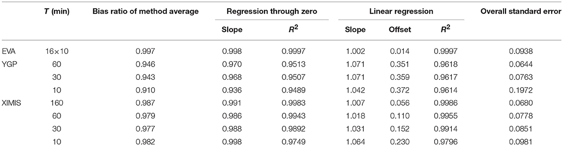
Table 2. Summary of method performance and variability.

The method variability is quantified by the overall standard errors in the furthest right column of Table 2. These were computed by taking the square root of the average squared COV for each tap. Here it is seen that the YGP method is the least variable because the moments of the data used by the method are inherently more stable than the extremes. XIMIS outperforms the industrial standard EVA method for T = 30 min, or longer.

Discussion of results

Non-Gaussian Characteristics

The essential difference between the Davenport peak factor method and extreme-value method is that the former estimates the distribution of extremes indirectly from the parent distribution, i.e., upwards from below, whereas the EVA method estimates directly from the extremes, i.e., downwards from above. The peak factor method assumes a Gaussian process, where the corresponding skewness is 0 and the kurtosis is 3. HPM corrects the peak factor for the non-Gaussian values of skewness and kurtosis on a tap-for-tap basis. The question to be answered is “how well does it succeed?”

The EVA methods make no assumption of Gaussian characteristics but require only that the epochal extremes are statistically independent. XIMIS additionally requires that the sub-epochal extremes follow a Poisson process, and this is ensured by the de-clustering procedure. The standard EVA and the XIMIS methods should be independent of skewness and kurtosis. Figure 13 shows the average method anomaly at each tap plotted against kurtosis for the EVA, XIMIS and YGP methods—there is no significant trend with kurtosis, but the degree of scatter is seen to be the least for EVA and the greatest for YGP.

FIGURE 13

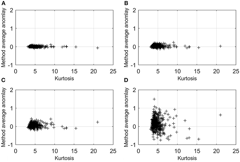
Figure 13. Kurtosis vs. Anomaly: (A) EVA N = 16 and T = 10 min (N_peak = 11), (B) XIMIS T = 160 min (N_peak = 11), (C) XIMIS T = 60 min (N_peak = 30), (D) YGP T = 60 min (N_peak = 30).

Equivalent Peak Factor

From the results presented in section Results, it became clear that the HPM methodology does perform poorly in comparison with direct EVA or XIMIS. The previous calibration of the Davenport peak-factor method (Cook, 1982b) attributed its insufficient accuracy to intermittency of the flow regime in the re-attachment zones behind the high-suction zones along the roof edges elevating the required peak factor value. The Hermite polynomial translation method should account for this by predicting the peak factor from the skewness and kurtosis. Figure 14 shows the Q-Q plot of the peak factor predicted by YGP and the datum value, back-calculated from the 78% datum (cross symbols). YGP values are 9% too low, on average, and the random scatter is very large. The solid circles denote the peak factors for datum suctions larger than Cp = −5, for which the YGP peak factors are 1% too large. Given that the YGP peak factor is conservative for the largest suctions, the deficiency for the smaller suctions may not seem important, but this deficiency applies to most of the roof area, so panel loads and overall uplift will be underestimated.

FIGURE 14

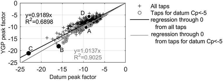
Figure 14. Q-Q plot of YGP peak factor vs. the equivalent datum peak factor.

Luo et al. (2016) conclude that “compared with HPM, XIMIS may indeed provide better estimations but it is more complicated and inconvenient to deal with many pressure taps.” While the derivation of both methods is very complex, the implementation of XIMIS is simple and requires similar number of steps to the one for YGP as shown in Table 1. The benefit to wind tunnel testing is that the record length for XIMIS can be reduced by a factor of six, and still the results remain better than HPM, on average.

The Role of Process Models

XIMIS is only an extreme value analysis method, not a process model. This study shows XIMIS to be superior to HPM (YGP) in this specific role. However, there are applications in which a process model is a requirement. One example is the non-linear response of tall buildings to wind loads for which a non-Gaussian process model for wind loading is needed to drive the non-linear equations of motion. As yet there is no better alternative for this than HPM. The calibration in this study helps establish the confidence that can be placed on it.

Conclusions

The XIMIS method, which uses the general penultimate distribution of extremes and was suggested for the peak wind speed estimation, was introduced as an alternative the peak wind pressure coefficient estimation. Its historical deviation through preceded studies, benefit and accuracy were summarized by presenting comparisons with commonly used and recent prevalent peak estimation methods, Gumbel extreme-value analysis and the Hermite-Davenport method of Yang et al. (2013), respectively. The main conclusions from the study are:

• The natural statistical variation between trials dominates over the differences between the methods.

• Conventional EVA using epoch maxima gives the most accurate estimates of peak suctions, but is inefficient in its use of the data, requiring significantly longer data records than YGP or XIMIS.

• The implementation of XIMIS is as simple as the one of YGP and remains more accurate than YGP even with data records six times shorter.

• The choice of record length for XIMIS is a compromise between accuracy and economy.

Author Contributions

NC performed the data analysis on two taps using excel, then EG performed the same analysis using Matlab to confirm the accuracy of the analysis before analyzing all taps. EG prepared most of figures and tables, and drafted the manuscript with input from NC. NC also drafted parts of the manuscript and provided valuable guidance in developing the paper including grammatical corrections.

Conflict of Interest Statement

The authors declare that the research was conducted in the absence of any commercial or financial relationships that could be construed as a potential conflict of interest.

Acknowledgments

This work is the result of unfunded curiosity-driven research. The assistance of Dr. Gregory A. Kopp in arranging access and permissions to use the Cp data is gratefully acknowledged.

References

Balderrama, J. A., Masters, F. J., Gurley, K. R., Prevatt, D. O., Aponte-Bermúdez, L. D., Reinhold, T. A., et al. (2011). The Florida Coastal Monitoring Program (FCMP): A review. J. Wind Eng. Ind. Aerodyn. 99, 979–995. doi: 10.1016/j.jweia.2011.07.002

CrossRef Full Text | Google Scholar

Brabson, B. B., and Palutikof, J. P. (2000). Tests for the Generalised Pareto distribution for predicting extreme wind speeds. J. Appl. Meteor. 39, 1627–1640. doi: 10.1175/1520-0450(2000)039/3C1627:TOTGPD/3E2.0.CO;2

CrossRef Full Text | Google Scholar

Chen, X., and Huang, G. (2009). Evaluation of peak resultant response for wind-excited tall buildings. Eng. Struct. 31, 858–868. doi: 10.1016/j.engstruct.2008.11.021

CrossRef Full Text | Google Scholar

Cook, N. J. (1982a). Towards better estimation of extreme winds. J. Wind Eng. Ind. Aerodyn. 9, 295–323. doi: 10.1016/0167-6105(82)90021-6

CrossRef Full Text | Google Scholar

Cook, N. J. (1982b). Calibration of the quasi-static and peak-factor approaches against the method of Cook and Mayne. J. Wind Eng. Ind. Aerodyn. 10, 315–341. doi: 10.1016/0167-6105(82)90005-8

CrossRef Full Text | Google Scholar

Cook, N. J. (2004). Confidence limits for extreme wind speeds in mixed climates. J. Wind Eng. Ind. Aerodyn. 92, 41–57. doi: 10.1016/j.jweia.2003.09.037

CrossRef Full Text | Google Scholar

Cook, N. J. (2012). Rebuttal of Problems on the extreme value analysis. Struct. Saf. 34, 418–423. doi: 10.1016/j.strusafe.2011.08.002

CrossRef Full Text | Google Scholar

Cook, N. J. (2016a). Short communication: on the Gaussian-Exponential Mixture Model for pressure coefficients. J. Wind Eng. Ind. Aerodyn. 153, 71–77. doi: 10.1016/j.jweia.2016.02.009

CrossRef Full Text | Google Scholar

Cook, N. J. (2016b). Discussion of Revisiting moment-based characterisation for wind pressures. J. Wind Eng. Ind. Aerodyn. 158, 155–161. doi: 10.1016/j.jweia.2016.09.001

CrossRef Full Text | Google Scholar

Cook, N. J., and Harris, R. I. (2004). Exact and general FTI penultimate distributions of extreme wind speeds drawn from tail-equivalent Weibull parents. Struct. Saf. 26, 391–420. doi: 10.1016/j.strusafe.2004.01.002

CrossRef Full Text | Google Scholar

Cook, N. J., Harris, R. I., and Whiting, R. (2003). Extreme wind speeds in mixed climates revisited. J. Wind Eng. Ind. Aerodyn. 91, 403–422. doi: 10.1016/S0167-6105(02)00397-5

CrossRef Full Text | Google Scholar

Cook, N. J., and Mayne, J. R. (1979). A novel working approach to the assessment of wind loads for equivalent static design. J. Wind. Eng. Ind. Aerodyn. 4, 149–164. doi: 10.1016/0167-6105(79)90043-6

CrossRef Full Text | Google Scholar

Cook, N. J., and Mayne, J. R. (1980). A refined working approach to the assessment of wind loads for equivalent static design. J. Wind. Eng. Ind. Aerodyn. 126, 11–23. doi: 10.1016/0167-6105(80)90026-4

CrossRef Full Text | Google Scholar

Davenport, A. G. (1964). Note on the distribution of the largest value of a random function with application to gust loading. Proc. Inst. Civil Eng. 28, 187–196. doi: 10.1680/iicep.1964.10112

CrossRef Full Text | Google Scholar

Ding, J., and Chen, X. (2014). Assessment of methods for extreme value analysis of non-Gaussian wind effects with short-term time history samples. Eng. Struct. 80, 75–88. doi: 10.1016/j.engstruct.2014.08.041

CrossRef Full Text | Google Scholar

Folgueras, P., Solari, S., Mier-Torrecilla, M., Doblaré, M., and Losada, M. A. (2016). The extended Davenport peak factor as an extreme-value estimation method for linear combinations of correlated non-Gaussian random variables. J. Wind Eng. Ind. Aerodyn. 157, 125–139. doi: 10.1016/j.jweia.2016.07.014

CrossRef Full Text | Google Scholar

Galambos, J., and Macri, N. (1999). Classical extreme value model and prediction of extreme winds. J. Struct. Eng. 125, 792–794.

Google Scholar

Gavanski, E., Gurley, K. R., and Kopp, G. A. (2016). Uncertainties in the estimation of local peak pressures on low-rise buildings by using the Gumbel distribution fitting approach. J. Struct. Eng. 142, 1–14. doi: 10.1061/(ASCE)ST.1943-541X.0001556

CrossRef Full Text | Google Scholar

Gringorten, I. I. (1963). A plotting rule for extreme probability paper. J. Geophys. Res. 68:813814.

Google Scholar

Gumbel, E. J. (1958). Statistics of Extremes. New York, NY: Columbia University Press.

Google Scholar

Harris, R. I. (1996). Gumbel revisited- a new look at extreme value statistics applied to wind speeds. J. Wind Eng. Ind. Aerodyn. 59, 1–22. doi: 10.1016/0167-6105(95)00029-1

CrossRef Full Text | Google Scholar

Harris, R. I. (1999). Improvements to the method of independent storms. J. Wind Eng. Ind. Aerodyn. 80, 1–30. doi: 10.1016/S0167-6105(98)00123-8

CrossRef Full Text | Google Scholar

Harris, R. I. (2001). The accuracy of design values predicted from extreme value analysis. J. Wind Eng. Ind. Aerodyn. 89, 153–164. doi: 10.1016/S0167-6105(00)00060-X

CrossRef Full Text | Google Scholar

Harris, R. I. (2006). Errors in GEV analysis of wind epoch maxima from Weibull parents. Wind Struct. 9, 179–191. doi: 10.12989/was.2006.9.3.179

CrossRef Full Text | Google Scholar

Harris, R. I. (2009). XIMIS, a penultimate extreme value method suitable for all types of wind climate. J. Wind Eng. Ind. Aerodyn. 97, 271–286. doi: 10.1016/j.jweia.2009.06.011

CrossRef Full Text | Google Scholar

Holmes, J. D., and Cochran, L. S. (2003). Probability distributions of extreme pressure coefficients. J. Wind. Eng. Ind. Aerodyn. 91, 893–901. doi: 10.1016/S0167-6105(03)00019-9

CrossRef Full Text | Google Scholar

Holmes, J. D., Melbourne, W. H., and Walker, G. R. (1989). A Commentary on the Australian Standard for Wind Loads. Part 2. Rep. No. AS 1170. Melbourne: Australian Wind Engineering Society.

Google Scholar

Holmes, J. D., and Moriarty, W. W. (1999). Application of the generalized Pareto distribution to extreme value analysis in wind engineering. J. Wind. Eng. Ind. Aerodyn. 83, 1–10. doi: 10.1016/S0167-6105(99)00056-2

CrossRef Full Text | Google Scholar

Hong, H. P., Li, S. H., and Mara, T. G. (2013). Performance of the generalized least squares method for the Gumbel distribution and its application to annual maximum wind speeds. J. Wind Eng. Ind. Aerodyn. 199:1210132. doi: 10.1016/j.jweia.2013.05.012

CrossRef Full Text | Google Scholar

Huang, G., Luo, Y., Gurley, K. R., and Ding, J. (2016). Revisiting moment-based characterization for wind pressures. J. Wind Eng. Ind. Aerodyn. 151, 158–168. doi: 10.1016/j.jweia.2016.02.006

CrossRef Full Text | Google Scholar

Huang, M. F., Lou, W., Chan, C. M., Lin, N., and Pan, X. (2013). Peak distributions and peak factors of wind-induced pressure processes on tall buildings. J. Eng. Mech. 139, 1744–1756. doi: 10.1061/(ASCE)EM.1943-7889.0000616

CrossRef Full Text | Google Scholar

Kareem, A., and Zhao, J. (1994). Analysis of non-gaussian surge response of tension leg platforms under wind loads. J. Offshore Mechanics Arctic Eng. 116, 137–144. doi: 10.1115/1.2920142

CrossRef Full Text | Google Scholar

Karpa, O., and Naess, A. (2013). Extreme value statistics of wind speed data by the ACER method. J. Wind Eng. Ind. Aerodyn. 112, 1–10. doi: 10.1016/j.jweia.2012.10.001

CrossRef Full Text | Google Scholar

Kasperski, M. (2003). Specification of the design wind load based on wind tunnel experiments. J. Wind. Eng. Ind. Aerodyn. 91, 527–541. doi: 10.1016/S0167-6105(02)00407-5

CrossRef Full Text | Google Scholar

Kopp, G. A., and Gavanski, E. (2010). Wind Tunnel Pressure Measurements on two FCMP Houses in Florida. Res. Rep. BLWT-5-2010. London, ON: The Boundary Layer Wind Tunnel Laboratory, Univ. of Western Ontario.

Google Scholar

Kwon, D. K., and Kareem, A. (2011). Peak factors for non-gaussian load effects revisited. J. Struct. Eng. 137, 1611–1619. doi: 10.1061/(ASCE)ST.1943-541X.0000412

CrossRef Full Text | Google Scholar

Lieblein, J. (1974). Efficient Methods of Extreme-Value Methodology. Rep. No. NBSIR 74-602. Washington, DC: National Bureau of Standards. doi: 10.6028/NBS.IR.74-602

CrossRef Full Text | Google Scholar

Liu, M., Chen, X., and Yang, Q. (2017). Estimation of peak factor of non-gaussian wind pressures by improved moment-based Hermite Model. J. Eng. Mech. 143:1233. doi: 10.1061/(ASCE)EM.1943-7889.0001233

CrossRef Full Text | Google Scholar

Luo, Y., Huang, G., Ding, J., and Gurley, K. R. (2016). Response to Revisiting moment-based characterization for wind pressures. J. Wind Eng. Ind. Aerodyn. 158, 162–163. doi: 10.1016/j.jweia.2016.08.012

CrossRef Full Text | Google Scholar

Ma, X., and Xu, F. (2017). Peak factor estimation of non-Gaussian wind pressure on high-rise buildings. Struct Design Tall Spec Build. 2017; 26:e1386. doi: 10.1002/tal.1386

CrossRef Full Text | Google Scholar

Peng, X., Yang, L., Gavanski, E., Gurley, K., and Prevatt, J. (2014). A comparison of methods to estimate peak wind loads on buildings. J. Wind. Eng. Ind. Aerodyn. 6, 125–137. doi: 10.1016/j.jweia.2013.12.013

CrossRef Full Text | Google Scholar

Peterka, J. A. (1983). Selection of local peak pressure coefficients for wind tunnel studies of buildings. J. Wind. Eng. Ind. Aerodyn. 13, 477–488. doi: 10.1016/0167-6105(83)90166-6

CrossRef Full Text | Google Scholar

Peterka, J. A., and Cermak, J. E. (1975). Wind pressures on buildings—probability densities. J. Struct. Div. ASCE 101,1255–1267.

Google Scholar

Sadek, F., and Simiu, E. (2002). Peak non-Gaussian wind effects for database-assisted low-rise building design. J. Eng. Mech. 128, 530–539. doi: 10.1061/(ASCE)0733-9399(2002)128:5(530)

CrossRef Full Text | Google Scholar

Simiu, E., and Heckert, N. A. (1996). Extreme wind distribution tails: a peaks over threshold approach. J. Struct. Eng. 122, 539–547. doi: 10.1061/(ASCE)0733-9445(1996)122:5(539)

CrossRef Full Text | Google Scholar

Song, J., Xu, W., Hu, G., Liang, S., and Tan, J. (2019). Non-Gaussian properties and their effects on extreme values of wind pressure on the roof of long-span structure. J. Wind. Eng. Ind. Aerodyn. 184, 106–115. doi: 10.1016/j.jweia.2018.11.027

CrossRef Full Text | Google Scholar

Stathopoulos, T. (1979). Turbulent Wind Action on Low Rise Buildings. PhD. Dissertation, London, ON: University of Western Ontario.

Google Scholar

Tieleman, H. W., Ge, Z., and Hajj, M. E. (2007). Theoretically estimated peak wind loads. J. Wind. Eng. Ind. Aerodyn. 95, 113–132. doi: 10.1016/j.jweia.2006.05.004

CrossRef Full Text | Google Scholar

Yang, L., Gurley, K. R., and Prevatt, D. O. (2013). Probabilistic modelling of wind pressure on low-rise buildings. J. Wind Eng. Ind. Aerodyn. 114, 18–26. doi: 10.1016/j.jweia.2012.12.014

CrossRef Full Text | Google Scholar