A Comparison of Strain-Based Methods for the Evaluation of the Relative Displacement of Beam-Like Structures

1. Introduction

The development and application of structural health monitoring (SHM) methods for bridges helps reduce and minimize the costs of inspection and maintenance of infrastructure and with the growing problem of aging infrastructure it can provide a means for evaluating the structural behavior over the life span of the structure. Displacement has been shown to be a useful parameter for evaluating the performance and health of the structure (Calvi and Kingsley, 1995; Ruiz-García and Miranda, 2003). Displacement is correlated with the strain and curvature of a structure, so any unusual behavior of the structure that alters the curvature is expected to affect the displacement of the structure. Either sudden or gradual changes in the displacement may indicate structural changes, damages, or deterioration. Additionally, displacement is frequently used as a serviceability design criteria because excessive displacements are uncomfortable to users and can cause damage to surround structures. In the United States, the American Society of Civil Engineers (ASCE) provides serviceability design requirements for buildings in ASCE/SEI 7-16 (American Society of Civil Engineers, 2017), the American Association of State Highway and Transportation Officials (AASHTO) provides serviceability limits for bridges (American Association of State Highway and Transportation Officials, 2010), the American Institute of Steel Construction (AISC) provides serviceability design guidelines for steel structures (American Institute of Steel Construction, 2011), and the American Concrete Institute (ACI) provides deflection limits for concrete structures (ACI 318R-11, 2011).

Several approaches can be used to determine the displacement which can be separated into two categories: direct measurement methods (contact and non-contact) and indirect measurement methods. Direct-contact based methods consist of linear variable differential transformers (LVDT's) (Merkle and Myers, 2004; Park et al., 2007), linear potentiometers (Corda and Al-Tayie, 2003), dial-gages, and hydrostatic systems (Marecos, 1978). To measure the displacement, these systems must be physically connected to the point of interest on the structure and be in contact with a stationary reference point. On a real structure, such as a bridge, these conditions may be challenging to find especially for bridges spanning over bodies of water or with high clearances. Non-contact direct measurement methods can be beneficial because they do not require direct access to the structure. Some of the non-contact direct monitoring methods that have been employed for displacement monitoring of a structure consist of global positioning systems (GPS) (Brown et al., 2006; Casciati and Fuggini, 2011), photogrammetry (Jáuregui et al., 2003), laser vibrometer (Nassif et al., 2005), radar interferometry (Gentile and Bernardini, 2008), and vision based methods (Lee and Shinozuka, 2006; Cigada et al., 2014; Ribeiro et al., 2014; Feng et al., 2015; Feng and Feng, 2016, 2018). These methods can be beneficial because they do not require pre-existing knowledge of the structure such as the boundary conditions. However, they still depend on a fixed reference point, GPS-based methods feature limited accuracy in the vertical direction, and the other above methods face various challenges when deployed for long term monitoring of a structure.

This is where measuring displacement indirectly can be beneficial, with methods using sensors such as accelerometers (Park et al., 2005), tilt sensors/inclinometers (Hou et al., 2005), or strain sensors (Foss and Haugse, 1995; Davis et al., 1996; Sigurdardottir et al., 2017). The benefit of using network of strain sensors to determine the displacement of a structure, is that the same sensor network can also be used to calculate other monitoring parameters such as the neutral axis (Sigurdardottir and Glisic, 2014), pre-stressing forces (Abdel-Jaber and Glisic, 2014), thermal signatures (Reilly and Glisic, 2018), and curvature (Kliewer and Glisic, 2017), and that is the reason why this research focuses on strain-based methods.

There are a variety of methods that can convert strain measurements into deformed shape (see section 2). The aim of this paper is to identify strengths and limitations of these various methods. These methods will focus on the relative displacement of the structure as opposed to the global displacement of the structure due to rigid body translation or rotations of the beam An overview of these methods is provided in the following section. The methods were compared in both dynamic and static tests for simply supported and cantilevered boundary conditions through applications to a numerical simulation and small-scale laboratory tests. The methods were also applied to an in-service highway overpass to evaluate the displacement serviceability limits. Fiber Bragg-grating strain sensors were used in all tests.

2. Strain to Displacement Methods

The strain to deformed shape methods considered in this paper are Newton-Cotes formulas (rectangle and trapezoidal rule), polynomial spline, strain-mode transformation, and curve fitting. An overview of these methods is given in this section. Readers that are familiar with these methods can skip this section, and move directly to section 3.

2.1. Newton-Cotes Formulas

2.1.1. Theoretical Background: Euler-Bernoulli Beam Theory

Following the assumptions of linear beam theory, the curvature in the cross-section of a beam, κ, can be determined using two strain measurements in parallel topology as represented in Equation (1):

$\begin{array}{ll}\kappa =\frac{{\epsilon }_b-{\epsilon }_t}{h}& (1)\end{array}$

where ε_b, ε_t and h are the strain at the bottom of the cross-section, the strain at the top of the cross-section and the distance between the sensors, respectively. Most common construction materials such as concrete, steel, and timber can be regarded as homogeneous at the macro-level (Glisic and Inaudi, 2008). In a beam-like structure made of homogeneous material, the curvature relates to the bending moment of beam:

$\begin{array}{ll}\kappa (x)=\frac{1}{r}=\frac{M}{EI}& (2)\end{array}$

where r, M, E, and I are the radius of curvature, the bending moment, Young's modulus, and the moment of inertia, respectively. The slope of a beam is equal to the derivative of the displacement and the curvature of a beam is equal to the negative double derivative of its displacement (Gere and Goodno, 2008):

$\begin{array}{ll}\kappa =-\frac{d^{2}v}{d{x}^2}& (3)\end{array}$

From Equation (3), the deflection of a beam can be found through the double integration of the curvature:

$\begin{array}{ll}v(x)=-{\displaystyle \int \int \kappa (x)dxdx+C_{1}x+C_2}& (4)\end{array}$

where C₁ and C₂ are constants of integration determined based on boundary conditions. For a simply supported beam the boundary conditions are v(0) = 0 and v(l) = 0, where l is the length of the beam. For displacement in a cantilevered beam, the boundary conditions are v(0) = 0 and θ(0) = 0, where θ is the slope of the beam. The deformed shape can be determined from Equation (4) by using the rectangle rule or the trapezoid rule (commonly known as Newton-Cotes quadrature). General strengths of these methods are that they are independent of the loading cases on the structure, require no assumptions of the distribution of curvature on the structure and can be applied to both static and dynamic strain data. This can be a very useful method for determining deformation when little is known about the structure and its loading conditions. While not widely present in the literature, these methods were applied by Sigurdardottir et al. (2017), where the static deformed shape of a pedestrian foot bridge was determined and provides explicit equations for the evaluation of the errors associated with numerical integration for evenly spaced sensors.

This paper will also present the use of the Newton-Cotes quadrature, where the quadrature points are fixed and the interpolating function is a polynomial with an order m (Bradie, 2006). The Newton-Cotes quadrature can be either closed, where the endpoints are included in the integration interval, or open, where the endpoints are not included in the integrating interval. Two types of Newton-Cotes formulas, the mid-point rectangular rule and the trapezoid rule, will be presented along with their application to determine the deformed shape from the curvature of a beam.

2.1.2. Rectangular Rule

The rectangular rule has an interpolation polynomial of order m = 0. It is the simplest open Newton-cotes formula. For a function f(x), on the interval [a, b], the rectangular rule is as follows:

$\begin{array}{ll}{\displaystyle {\int }_a^b}f(x)dx\approx (b-a)f(\frac{a+b}{2})& (5)\end{array}$

To expand the rectangular rule to a beam with curvature values known curvature values at more than two locations, the composite Newton-Cotes quadrature is used. The structure consists of n sub-intervals along the length of the beam, as shown in Figure 1, with n + 1 known curvature values. The rectangular rule, Equation (5), is applied to each sub-interval [x_i−1, x_i], and the following equation is obtained:

$\begin{array}{l}{\displaystyle {\int }_{x_0}^{x_n}}f(x)dx\approx {\displaystyle \sum _{i=1}^n}{\displaystyle {\int }_{x_{i-1}}^{x_i}}f(x)dx+C_1\\ ={\displaystyle \sum _{i=1}^n}(x_i-x_{i-1})f(\frac{x_i+x_{i-1}}{2})+C_1& (6)\end{array}$

FIGURE 1

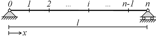
Figure 1. Beam, with length l, equipped with sensors at n+1 locations (cross-sections) providing known curvature values at each locations (κ(X₀), κ(X₁), ⋯, κ(X_n)).

2.1.3. Trapezoid Rule

The trapezoid rule has an interpolation polynomial of order m=1 and is the simplest closed Newton-Cotes formula. For a function f(x), on the interval [a, b], the trapezoid rule is as follows:

$\begin{array}{ll}{\displaystyle {\int }_a^b}f(x)dx\approx (b-a)(\frac{f(a)+f(b)}{2})+C_1& (7)\end{array}$

Similar to the rectangular rule, Equation (7) is the integration for one sub-interval. The composite trapezoid rule is used to determine to apply the method to a beam with more than one sub-interval:

$\begin{array}{l}{\displaystyle {\int }_{x_0}^{x_n}}f(x)dx\approx {\displaystyle \sum _{i=1}^n}{\displaystyle {\int }_{x_{i-1}}^{x_i}}f(x)dx+C_1\\ =\frac{1}{2}{\displaystyle \sum _{i=1}^n}(x_i-x_{i-1})(f(x_{i-1})+f(x_i))+C_1& (8)\end{array}$

From Equation (4), an expression for the deformed shape of the beam at sensor location x_i, can be found by applying the rectangular integration rule in Equation (6) or applying the trapezoid integration rules in Equation (8) twice to the curvature, κ(x_i). In the case where the distances between sensors are equal, Δx = l/n for all sub-intervals, simplified expression for the deformed shape from the rectangular and trapezoid rules were found by Sigurdardottir et al. (2017).

2.2. Polynomial Spline

This method estimates the displacement of a beam by fitting a quadratic curve to each set of neighboring triplet of points. This method is related to the Simpson's rule, a second order Newton Cote's quadrature rule where the data points must be equally spaced. However, this method is applicable to structures with irregular sensor spacing and preserves the number of measurement points, providing displacement estimates at each sensor location, rather than reducing the number of estimation points with each round of integration as the Simpson's rule does. This is particularly important as a structure may be sparsely instrumented and strain to displacement transformation requires double integration. In a structure with a continuously smooth curvature curve, this method is expected to provide more accurate results compared to numerical integration with the trapezoid and rectangular rule for beam-like structures without linear curvature distributions.

An application of this method was introduced by Kirby et al. (1997) and applied to a composite tubular cantilever instrumented with foil strain gages. Their experimental tests showed estimating with quadratic curvature may improve the displacement estimation and suggested the error in the method could be improved with the use of FBG strain sensors.

For this method, the beam must be instrumented with an odd number of sensors greater than or equal to three. The beam is divided into segments of three adjacent sensor locations, creating a total of m = (n − 1)/2 segments, where n is the number of sensor locations and m is the number of segments. At the boundary between each segment, the continuity conditions for the slope and displacement are preserved. For each segment, i, a second order polynomial is fit to the three curvature values. With three curvature values and three unknowns, the coefficients of polynomials A₁, B₁, and C₁ can be obtained directly without needing regression analysis such as the method of least squares. There is a system of equations for the curvature of each beam segment can be defined in matrix form as:

$\begin{array}{ll}\kappa =\text{x}\alpha & (9)\end{array}$

where the measured curvature vector is κ$={\left\{{\kappa }_{1,1},{\kappa }_{1,2},{\kappa }_{1,3},\cdots ,{\kappa }_{i,3}\right\}}^T$, the fitting parameters are $\alpha ={\left\{A_1,B_1,C_1,\cdots ,A_m,B_m,C_m\right\}}^T$, and a matrix for the sensor coordinates, x is defined as:

$\begin{array}{ll}\text{x}=\left[\begin{array}{ccc}{x}_{1,1}^2& x_{1,1}& 1\\ x_{1,2}^2& x_{1,2}& 1\\ x_{1,3}^2& x_{1,3}& 1\\ ⋮& ⋮& ⋮\\ x_{m,j}^2& x_{m,j}& 1\end{array}\right]& (10)\end{array}$

Using the known values for κ and x, the fitting parameters can be found with α =x⁻¹κ. With double integration, equations for the slope, Equation (26), and displacement, Equation (27), for each segment can be found. The constants of integration, D_i and E_i, are found using the continuity conditions between each segment and the boundary conditions at the ends of the beam (see Equations 11 and 12). For adjacent segments:

$\begin{array}{ll}{\theta }_i(x_{i,3})={\theta }_{i+1}(x_{i+1,1})& (11)\end{array}$

$\begin{array}{ll}{y}_i(x_{i,3})=y_{i+1}(x_{i+1,1})& (12)\end{array}$

Another system of equations is created using these conditions and solving for the constants of integration for each segment, i. From this method, the displacement at each sensor location can be determined or a continuous displacement curve for every location of the beam can be found. This method is applicable to both static and dynamic beam systems, where it is repeated at each time-step for dynamic cases.

2.3. Strain Mode Transformation

A commonly used method for strain to displacement transformation is strain mode transformation (SMT). This method was initially introduced by Foss and Haugse (1995) and there have been numerous applications of this method since then. Shin et al. (2012) provided an evaluation of the SMT method, with application to a railroad bridge, a suspension bridge and a multi-girder simple span bridge. Based on analysis presented in that literature, the use of a scale factor from a controlled field test is proposed, as opposed to a geometric constant for actual structures. Kang et al. (2007) presented an application of the SMT method to an aluminum and an acrylic beam instrumented with FBG strain sensors. While this method is typically applied only in dynamic monitoring, Bogert et al. (2003) presented a static analysis of the SMT method with an application to a small-scale laboratory test. Rapp et al. (2009) expands the SMT method to a two-dimensional structure for estimating the displacement field. This method relies on modal analysis to translate strain to displacement. The transverse vibration displacement, y(x_i), of a beam can be represented by modal superposition:

$\begin{array}{ll}{y}_i(t)=[{\varphi }_{ij}]\{q_j(t)\}& (13)\end{array}$

where ϕ_ij is the modal displacement and q_j(t) are the generalized coordinates. From beam theory, the strain at any location on the beam is equivalent to the following expression:

$\begin{array}{ll}{ϵ}_i(t)=y_c[{\varphi }_{ij}^{″}]\{q_j(t)\}& (14)\end{array}$

where y_c is the distance from the neutral axis to the strain sensor, ${\varphi }_{ij}^{″}$ is the curvature of the modal displacement ϕ_ij. From Equation (14), the modal coordinates, {q_j(t)}, are approximated using the least squares method:

$\begin{array}{ll}\{q_j(t)\}={[{[{\varphi }_{ij}^{″}]}^T[{\varphi }_{ij}^{″}]]}^{-1}{[{\varphi }_{ij}^{″}]}^T\{{ϵ}_i(t)\}& (15)\end{array}$

Substituting Equation (15) into Equation (13), an equation for the modal displacement is obtained:

$\begin{array}{ll}{y}_i(t)=[{\varphi }_{ij}]{[{[{\varphi }_{ij}^{″}]}^T[{\varphi }_{ij}^{″}]]}^{-1}{[{\varphi }_{ij}^{″}]}^T\{{ϵ}_i(t)\}& (16)\end{array}$

For the SMT method, the number of modes, n, is limited by the number of sensors on the beam, m, where m ≥ n. The modal displacement matrix must be determined for the beam to implement the SMT method. This requires some assumptions about the structure to be made, unlike the numerical integration methods presented in section 2.1. If the behavior or loading of the structure is unknown, this can be a limitation of this method. There are several approaches that can be used to obtain the modal coordinate matrix. The strain modes can be obtained from a finite element model (FEM) of the beam and is the more common approach for this method with applications presented by Foss and Haugse (1995); Bogert et al. (2003); Kang et al. (2007); Derkevorkian et al. (2013). A drawback of using a FEM to determine the modal coordinate matrix is that developing an accurate model of the structure can be time intensive and computationally expensive. Wang et al. (2014) presented a new method for determining the modal coordinated using the strain response rather than relying on a numerical model. The modal coordinate matrix can also be determined using theoretical mode shapes, such as the approach presented by Shin et al. (2012). This is the method that will be used in this paper. Using Euler-Bernoulli beam theory, the theoretical mode shapes and theoretical curvature shapes for a simply supported beam are:

$\begin{array}{ll}{\varphi }_{ij}=sin\frac{j\pi x_i}{l}& (17)\end{array}$

$\begin{array}{l}{\varphi }_{ij}^{″}=-{(\frac{j\pi }{l})}^{2}sin\frac{j\pi x_i}{l}\\ =-{(\frac{j\pi }{l})}^2{\varphi }_{ij}& (18)\end{array}$

where l is the length of the beam. Similarly, using Euler beam theory, the theoretical mode shapes and curvature shapes for a cantilevered beam can be determined (Young et al., 1949; Leissa and Qatu, 2011):

$\begin{array}{ll}{\varphi }_{ij}=cosh({\beta }_j{x}_i)-cos({\beta }_j{x}_i)-{\gamma }_j(sinh({\beta }_j{x}_i)-sin({\beta }_j{x}_i))& (19)\end{array}$

$\begin{array}{ll}{\varphi }_{ij}^{″}={\beta }_j^2[cosh({\beta }_j{x}_i)+cos({\beta }_j{x}_i)-{\gamma }_j(sinh({\beta }_j{x}_i)+sinh({\beta }_j{x}_i))]& (20)\end{array}$

Where γ_j and β_j are:

$\begin{array}{ll}{\gamma }_j=\left\{0.73410,1.01847,0.99922,1.000,\cdots \right\}& (21)\end{array}$

$\begin{array}{ll}{\beta }_{j}l=\left\{1.875,4.494,7.855,(2*j-1)\pi /2,\cdots \right\}& (22)\end{array}$

This method will be applied to both laboratory tests and to an in-service highway overpass and the results will be presented in later sections.

2.4. Curve Fitting

This method determines the relative displacement curve of the structure by performing regression analysis on the discrete curvature data points to fit an equation (i.e., interpolate the curvature distribution along the beam with an equation). The double integration of that fit curve is performed which provides the displacement curve of the beam. This method was utilized by Kim and Cho (2004) to estimate the deflection of a simply supported beam subjected to a static point load by fitting a first order polynomial expression and compared the performance of the method to dial strain gages. Xu et al. (2015) fit higher order polynomial equations using the method of least squares to obtain the coefficients, applying the method to dynamic numerical test and static load tests. Vurpillot et al. (1996) used quadratic equations fit to the curvature of a continuous beam and found the displacement for each segment of the structure.

Unlike the Newton-Cotes formulas, this method requires some assumptions to be made of the curvature curve profile in order to determine what fitting function to use for the structure. One method is to use a harmonic equation, such as the general modal equation for a beam under any boundary conditions or loading conditions:

$\begin{array}{l}{\varphi }_j(x_i)=C_{1}sin({\beta }_j{x}_i)+C_{2}sinh({\beta }_j{x}_i)\\ +C_{3}cos({\beta }_j{x}_i)+C_{4}cosh({\beta }_j{x}_i)& (23)\end{array}$

where C1–C4 and α are constants. From Equation (23) an equation for the curvature of the beam is found and can be fit to the discrete curvature data points for a structure:

$\begin{array}{l}{\kappa }_j(x_i)=-{\beta }_j{x}_i^2(-C_{1}sin({\beta }_j{x}_i)+C_{2}sinh({\beta }_j{x}_i)\\ -C_{3}cos({\beta }_j{x}_i)+C_{4}cosh({\beta }_j{x}_i))& (24)\end{array}$

If assumptions are made regarding the boundary conditions of the beam, these equations become simplified to Equation (17) for a simply supported beam and Equation (19) for a cantilevered beam. Another method is to assume the curvature takes the shape of a quadratic curve (e.g., due to a linearly distributed load) and approximate the curvature using a second order polynomial:

$\begin{array}{ll}\kappa (x)=A{x}^2+Bx+C& (25)\end{array}$

Which, yields approximations for the slope and displacement upon double integration:

$\begin{array}{ll}\theta (x)=-(\frac{1}{3}A{x}^3+\frac{1}{2}B{x}^2+Cx+D)& (26)\end{array}$

$\begin{array}{ll}y(x)=-(\frac{1}{12}A{x}^4+\frac{1}{6}B{x}^3+\frac{1}{2}C{x}^2+Dx+E)& (27)\end{array}$

Where A, B, and C are the fitting parameters determined by curve fitting and the constants D and E can be determined based on the boundary conditions. In the case where linear curvature is assumed, a first order polynomial can be used as opposed to Equation (25).

Using the method of least squares to minimize the error between the predicted curvature values from Equation (25) and the curvature data points, the best fit line can be found. The values for A, B, and C can then be input into Equation (27) to find the predicted displacement curve. This method applies to both static and dynamic beam loading cases, where it is repeated at each time-step for dynamic cases.

From the mathematical point of view, the relationship between curvature and shape of a line (e.g., centroid line of a beam) is defined by the formula:

$\begin{array}{ll}k(x)=y^{″}/(1+{y^{\prime }}^2)\ast 3/2& (28)\end{array}$

where ′ denotes the first and ″ the second derivative over x. Any line belonging to a geometrical plane (e.g., centroid plane of a plate structure) or spatial two-dimensional manifold (e.g., centroid manifold of a shell) would have the same relationship between the curvature and shape. Given that in the linear theory of beams the deformations (strain and shear strain) and displacements (including rotations) are small, y′ term in the above expression can be neglected, curvature becomes simply the second derivative of deformed shape (i.e., k(x) = y″), and deformed shape can be found as double integral of curvature. Thus, the applicability of methods discussed in this paper can be expanded from beam-like structures to other structures, such as plates and shells, as long as they behave under the assumptions of small deformations and displacements.

3. Analytical and Numerical Simulations

To evaluate the errors of the shape estimation algorithms presented in the previous section, numerical simulations were performed. The assumptions made in the different methods, for example a method using linear curvature assumption vs. a quadratic curvature assumption, can introduce different levels of error into the displacement estimation depending on the beams loading conditions. To compare the errors for these different methods, the following section will compare the estimated displacement from strain to the displacement for several different numerical test cases. Four different static load and boundary condition cases were evaluated using linear beam theory. The displacement estimation methods were also evaluated using a finite element model of two dynamic cases, a cantilever beam and a simply supported beam.

The aim of this section is to estimate inherent (theoretical) error of each integration method for different sensor configurations, and typical boundary conditions and loads. Hence, the methods are compared with analytical and/or numerical models rather than to real (experimental) displacement measurements in order to exclude from analysis the epistemic error of linear theory, which is unknown. Comparison with experimental data is performed in sections 4 and 5.

3.1. Static Analytical Simulations

A total of four different static analytical simulations were done to evaluate the performance of the different shape estimation algorithms as shown in Figure 2: a cantilever beam modeled with a point load at the free end, which results in a linear curvature profile; a simply supported beam with a point load at the center, which has a broken-linear curvature profile; a cantilever beam with a uniform distributed load, which has a quadratic curvature profile; and a simply supported beam with a load increasing uniformly to one end, which results in a cubic curvature profile. This choice of simulations was made to cover a variety of boundary conditions and load cases.

FIGURE 2

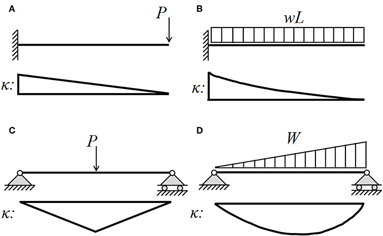
Figure 2. Static numerical simulation loading conditions and curvature profiles: (A) cantilever with point load-linear, (B) simply supported with central point load- broken linear, (C) cantilever with uniform distributed load-quadratic, and (D) simply supported with uniformly increasing distributed load-cubic.

A dimensionless analysis was performed, independent of the load, stiffness or length of the beam and assuming a uniform cross-section. The equations for the curvature for each boundary condition and loading case can be rearranged to include the parameter x_n = x/L, representing the dimensionless location along the beam and isolating all other parameters as shown in the following equations:cantilever beam with point load:

$\begin{array}{ll}\kappa =\frac{P}{EI}(L-x)=\frac{PL}{EI}*(1-x_n)& (29)\end{array}$

cantilever beam with uniformly distributed load:

$\begin{array}{ll}\kappa =\frac{w}{2EI}{(L-x)}^2=\frac{w{L}^2}{2EI}*{(1-x_n)}^2& (30)\end{array}$

simply-supported beam with central point load:

$\begin{array}{ll}\kappa =\frac{P}{2EI}(x)=\frac{PL}{2EI}*(x_n)& (31)\end{array}$

and simply-supported beam with uniformly increasing distributed load:

$\begin{array}{ll}\kappa =\frac{Wx}{3EI*L^2}(L^2-x^2)=\frac{WL}{3EI}*(x_n-x_n^3)& (32)\end{array}$

From Equation (4), the displacement is equal to the double integral of the curvature. To perform the dimensionless analysis, the initial term in the curvature equations is a constant, consisting of a combination of W, P, E, I, and L, and independent of the location on the beam so it can be removed from the integration as a constant. For the analysis, the curvature and displacement were calculated at evenly spaced intervals, simulating a structure instrumented with evenly spaced strain sensors. To observe the effects the number of sensors has on the error of the methods, four different sensor configurations were explored: 5, 7, 9, and 11 evenly spaced locations including both ends of the beam.

For each case, using the moment distribution from the applied loads, the curvature of the beam was found at evenly spaced locations on the beam. The displacement was then approximated from the curvature values using four different strain to displacement transformation methods: rectangular rule trapezoid rule, curve fitting, and the cubic spline method. The strain modal transformation method was not used for these cases because they are static conditions. The actual displacement for each case was determined directly from the loading cases using linear beam theory. The results for the displacement analysis for the case with seven sensor locations is shown in Figure 3, where C is the constant term in Equations (29–32).

FIGURE 3

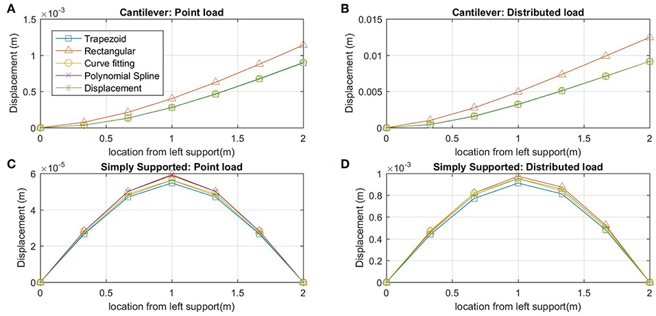
Figure 3. Dimensionless displacement estimations from static beam theory analysis for beam with 7 sensor locations: (A) cantilever with point load, (B) cantilever with uniform distributed load, (C) simply supported with central point load, and (D) simply supported with uniformly increasing distributed load.

The methods were evaluated using the normalized root mean square (RMS) error, as shown in Equation (33).

$\begin{array}{ll}RMS=\frac{\sqrt{\frac{1}{n}{\displaystyle {\sum }_{i=i}^n}{(y_i-\widehat{y_i})}^2}}{max(y)}& (33)\end{array}$

where $\widehat{y_i}$ is the estimated displacement, y_i is the measured displacement, and n,is the number of sensor locations. The results with the RMS error for the static analysis for each sensor configuration is shown in Table 1. It is important to note, these error values only include the error inherent to the method, no other errors are included such as sensor noise or epistemic error of model (beam theory).

TABLE 1

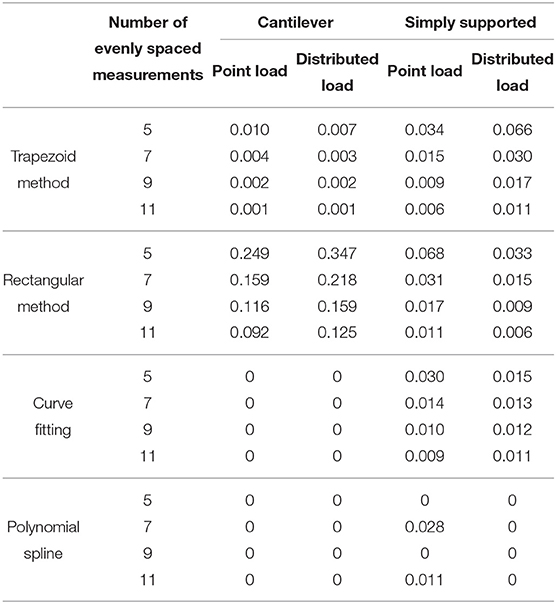
Table 1. RMS for static displacement analysis with evenly spaced measurements.

The results show that for all cases, other than the simply supported beam with a distributed load, the rectangular rule had the worst performance for calculating the vertical displacement with the highest RMS error. For most cases, the polynomial spline has the smallest error. However, for the simply supported beam with a central point load this is not always the case. As the number of sensors on the beam increases, the RMS error does not decrease. The results show that for the analysis with 7 and 11 sensors, the error is much higher than the analysis with 5 and 9 sensors. This is because the beam has a broken-linear curvature distributions so when the point load on the beam is located in the middle of a segment the error is higher than when the point load is located at the boundary of two segments. If the loading conditions are known for the structure, this can help guide in the selection of the method to use for the analysis. The curve fitting method had the second lowest error for most beam cases. The results also show that as the number of sensors on the beam increase, the RMS error decreases for most cases. However, for the curve fitting method and the cubic spline method, for the cantilever beam the number of sensors used does not impact the RMS error substantially. With only 5 sensor locations, both the curve fitting and cubic spline methods provide exact estimations of the displacement for a cantilever beam as the curvature for the given loads is either linear or parabolic. The same is seen for the cubic spline method for the simply supported beam with a distributed load. In this case the curvature is cubic, so cubic spline will make minimal errors.

In a real-life application, sensors are not likely to be installed with equal spacing. There may be limitation, such as accessibility to the structure, that limit the possible locations a sensor can be installed. Because of these limitations, the previous four static loading cases were repeated for a beam with uneven sensor spacing. The curvature and displacement were calculated at seven different location along the beam at the following locations: {0, 0.125, 0.375, 0.5, 0.625, 0.75, 1}*L, with increased spacing between locations 2 and 3 and locations 6 and 7. The RMS error for this analysis is shown in Table 1.

As expected, the error values for all methods increased compared to the analysis with evenly spaced sensors. Overall, the cubic spline method introduces the lowest levels of error when the sensors are unequally spaced and the rectangular method has the highest error for all cases other than the simply supported beam with a point load where the trapezoid method has the highest error.

3.2. Dynamic Numerical Simulations

For the dynamic numerical simulations, a finite element analysis (FEA) was performed in ANSYS for both a simply supported beam and a cantilevered beam. The beam modeled was 1.6 m long, a width of 0.25 m and a height of 0.01 m. The beam dimensions and the number of sensors used in this analysis were selected based on the dimensions used in a small-scale experimental test, see section 4, allowing for easier comparison between the numerical simulations and laboratory tests. A transient analysis was performed on the beam with both cantilevered and simply supported boundary conditions. An arbitrarily acceleration time-history, shown in Figure 4A, was applied to the structure.

FIGURE 4

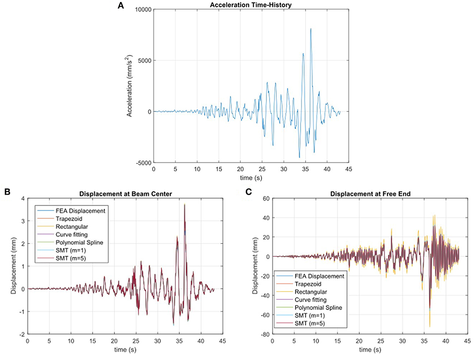
Figure 4. (A) Acceleration time-history applied to the FEA beam model, modified from PEER (2013), (B) Center displacement for FEA transient analysis of a simply supported beam, and (C) Free end displacement for FEA transient analysis of a cantilever beam.

The resulting surface strains and vertical displacement at the neutral axis were recorded for seven equally spaced locations along the beam for both of the FEA cases. At each measurement location, the displacement was calculated from the strain measurements using the methods introduced in the previous section. The resulting displacement at the center of the simply supported beam is shown in Figure 4B and the resulting displacement at the free end of the cantilever beam is shown in Figure 4C.

To evaluate the performance of the displacement estimation methods, the normalized root mean square (RMS) error, Equation (33), and the Pearson's coefficient of correlation (ρ), Equation (34), were found for each measurement location. The Pearson correlation coefficient is a measure of the linear correlation between two variables and has a value ranging from –1 to +1, where 0 is no linear correlation and +1 is a total positive linear correlation.

$\begin{array}{ll}{\rho }_j=\frac{{\displaystyle {\sum }_{i=1}^n}(y_{j,i}-{\overline{y}}_j)(\widehat{y_{j,i}}-{\bar{\widehat{y}}}_j)}{\sqrt{{\displaystyle {\sum }_{i=1}^n}{(y_{j,i}-{\overline{y}}_j)}^2{(\widehat{y_{j,i}}-{\bar{\widehat{y}}}_j)}^2}}& (34)\end{array}$

where ρ_j is the Pearson correlation at location j, ŷ_{j, i} is the estimated displacement at time i, y_{i, j} is the measured displacement,ȳ_j is the mean of the measured displacement at location j, and n is the number of sensor locations. The results for the simply supported beam analysis are shown in Figures 5A,B.

FIGURE 5

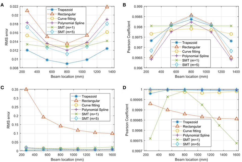
Figure 5. (A) RMS error and (B) Pearson coefficient for the estimated displacement compared to actual displacement for a FEA transient analysis of a simply supported beam and (C) RMS error and (D) Pearson coefficient for the estimated displacement compared to actual displacement for a FEA transient analysis of a cantilever beam.

For the simply supported beam, the highest errors were observed at the first and the last instrumented cross-section. Overall, the rectangular method had the highest RMS error for all sensor locations. The polynomial spline method had the second highest errors and the lowest Pearson coefficient for all locations other than the mid-span of the beam. Overall, the trapezoid method has the lowest RMS error for all locations. At the center for the beam, the SMT method with m = 5 has the second lowest RMS error and the second highest Pearson coefficient. For the simply supported beam, the performance of the other methods varies depending on the location on the beam. For applications where higher accuracy is desired at a specific location, the method with best performance at the desired location can be used.

For the cantilever beam analysis, the rectangular method has the worst performance for determining the beam displacement with RMS errors significantly higher than any of the other methods. These results for the cantilevered beam analysis are shown in Figures 5C,D. The SMT method with m = 1 had the second worst performance compared to all the other methods, with a higher RMS error and the lowest Pearson coefficient at the ends of the beam. This is likely because the SMT method with m = 1 is only estimating the first modal shape so when additional modes in the beam are excited, the method is unable to accurately estimate the displacement. Alternatively, the SMT method with m = 5 performs very well for estimating the displacement with the second lowest RMS errors and a very high Pearson coefficient at all measurement locations on the beam. The polynomial spline method has the lowest RMS errors for most locations on the beam with a very high Pearson coefficient >0.999.

The studies presented in this section show that the error of each method depends on number of sensors, their location on the structure, the load case, and boundary conditions of the beam. As a consequence, it is practically impossible to propose generalized formulas for prediction of error that may cover all possible load cases, boundary conditions and configurations of sensors (especially if the sensors are not equidistantly spaced). Thus, in case of more complex cases than those presented above, a specific error analysis should be performed taking into account specific load cases, boundary conditions and sensor configuration. However, this analysis can follow the workflow presented in this section.

4. Experimental Testing

In the previous section, analytical, and numerical modeling helped assess the theoretical performance of the considered methods and confirmed their potential applicability. However, considerations in previous section ignored epistemic errors related to linear theory, as well as the errors associated to the monitoring system. That is the reason why in this section the methods are evaluated through laboratory testing. The strain to displacement methods discussed in the previous sections were applied to an aluminum beam in small scale laboratory testing. For the experimental tests, the beam was tested with both simply-supported and cantilevered boundary conditions. The beam was instrumented with five fiber Bragg grating (FBG) fiber-optic sensors along the top surface of the beam. The FBG sensors have a gage length of 10 cm and are equally spaced at 10 cm apart. The beam is 0.95 cm thick, 25.4 cm wide, and the length of the beam between supports is shown in Figure 6. There are a total of 5 FBG strain sensors installed on the aluminum beam. The sensors are spaced 20 cm apart, center-to-center with the first FBG sensor located at 62.5 cm for the simply supported condition and at 39.5 cm for the cantilever, measured from the left beam support.

FIGURE 6

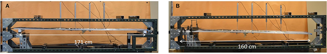
Figure 6. Experimental set up for aluminum beam laboratory tests with simply-supported (A) and cantilever (B) boundary conditions.

Assuming linear beam theory, when there are no normal forces, the strain in the cross-section is anti-symmetric about the neutral axis. Based on this assumption, the strain at the bottom of the beam is equal and opposite to the strain measured at the top of the beam and the curvature at each sensor location can be found using Equation (1). To provide a direct comparison, four LVDT displacement sensors were installed, measuring the displacement of the top surface of the beam. The LVDT sensors are shown in Figure 6 and their position aligns with the center of the FBG sensors. For the simply supported beam tests, the 4 LVDT sensors are aligned with FBG sensors 1–4 and for the cantilever beam tests, the 4 LVDT sensors are aligned with FBG sensors 2–5. The experimental set up for the aluminum beam is shown in Figure 6. The number of sensors and he number of LVDTs were chosen based on availability and budget constraints.

The beam was tested under both static and dynamic loading conditions. For all cases, the strain response from the FBG sensors and the displacement response from the LVDT sensors was obtained. A sampling rate of 250 Hz was used for both the FBG and LVDT data collection. The following sections will describe the loading cases and the provide the experimental results.

4.1. Simply Supported Beam

Both static and dynamic loading cases were applied to the simply supported beam. Static load tests consisted of a 11.69 N point load applied at the center of the beam and the measurements were taken with the FBG strain sensors and the LVDT displacement sensors. From the strain measurements the curvatures were calculated using Equation (1). From the curvature values, the displacement was calculated using each of the strain based displacement methods. The results are shown in Figure 7. As shown in the figure, all four methods are in good agreement with the displacement measurements from the LVDT sensor results, with the polynomial spline and the rectangular methods overestimating the displacement and the trapezoid and curve fitting methods underestimating the displacement. The RMS error for each of the methods at each sensor location was also determined. For the center of the beam, the rectangular method had the lowest error and the Trapezoid method had the worst performance with the highest RMS error for all locations. Overall, all methods performed well for estimating the displacement with a maximum error <6% and a minimum error of 2.5%. The differences observed in the experimental testing compared to the analytical estimation are likely attributed to epistemic error of the linear theory and errors associated to monitoring system such as repeatability, installation/strain transfer, and gauge length.

FIGURE 7

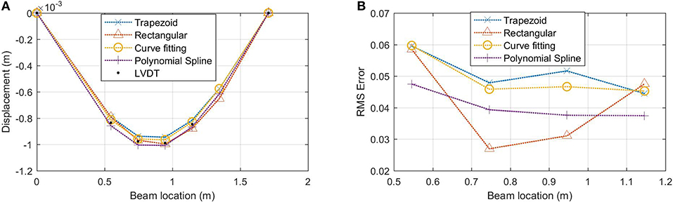
Figure 7. Simply supported beam experimental tests with a point load at the mid-span (A) displacement from FBG and LVDT sensors and (B) RMS error of strain based displacement estimations at each sensor location.

Dynamic free vibration experimental tests were performed on the simply supported beam by displacing the beam at the mid-span and releasing to induce a time-period of free vibration. A total of 10 free vibration tests were done on the beam. For each test, the displacement was determined from the FBG strain response and compared with the displacement measurements from the LVDT sensors. An example of the displacement at the mid-span of the beam for one time segment is shown in Figure 8A. These results are typical for the displacement results for all of the tests and measurement locations, showing there is good agreement between the LVDT displacement and the displacement calculated based on the strain. To evaluate the performance of these methods, the RMS error and the Pearson coefficient were calculated and are shown in Figures 8B,C. For the free vibration tests, the errors observed for the methods were similar in magnitude to the errors observed for the static tests with a maximum error <6.5% and a minimum error of 2.5%. The trapezoid method had the highest RMS error and the curve fitting method had the lowest Pearson coefficient whereas the SMT method had the lowest errors and highest Pearson coefficients. Similarly, differences between the experimental testing compared to the analytical estimation may be attributed to epistemic error of the linear theory and errors associated to monitoring system.

FIGURE 8

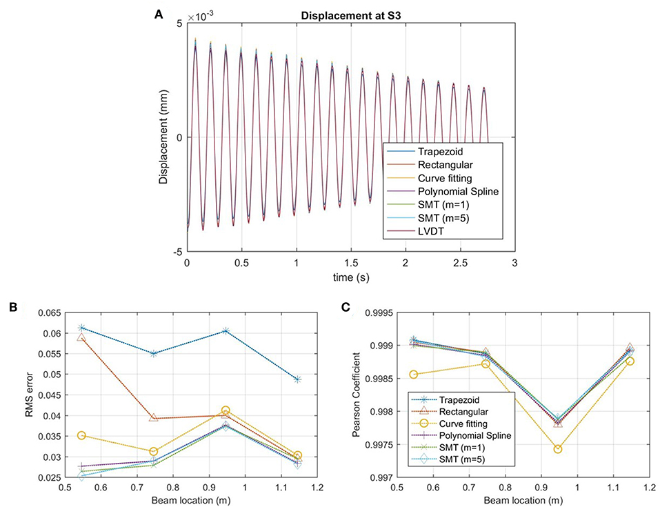
Figure 8. Experimental free vibration results: (A) displacement at mid-span of simply supported beam, (B) RMS error, and (C) Pearson coefficient.

Additional dynamic tests were performed on the simply supported beam with random impact loading. A total of 10 random impact tests were performed by using a hammer to randomly impact the beam for a 45 s time period. The resulting FBG strain response and LVDT displacement response were recorded. An example of the displacement at the mid-span from a time segment of one of the impact tests is shown in Figure 9A. This figure shows that there is good agreement between the LVDT displacement and the calculated displacement methods. However, due to the limitations of the LVDT sensor it does not record the higher frequency displacements, as illustrated at the displacement peaks in Figure 9, that the displacement results from the strain sensors are able to record. This is confirmed when a fast Fourier transformation(FFT) is performed on the FBG strain response and the LVDT displacement response. The frequency domain for the FBG response shows the first four natural frequencies whereas the frequency domain for the LVDT sensors only clearly shows the first two natural frequencies. Because of this, RMS errors are higher and the Pearson coefficients are lower compared to the previous experimental results presents, as shown in Figures 9B,C. The highest errors are located closer to the left end of the beam with a maximum error of 17% and the lowest errors are located on the right end of the beam with errors >7%. Overall, the polynomial spline having the best performance of the methods with the lowest RMS error at 3 of the 4 sensor locations.

FIGURE 9

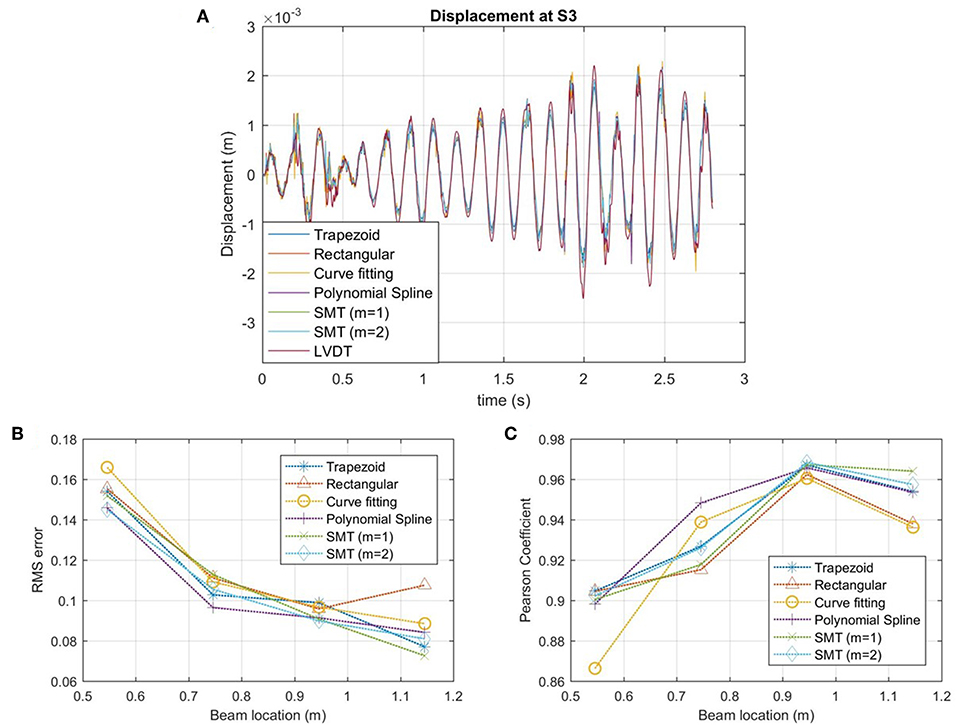
Figure 9. Random impact dynamic test (A) displacement response at mid-span of simply supported beam, (B) RMS error, and (C) Pearson coefficient.

4.2. Cantilever Beam

Both static and dynamic loading cases were applied to the cantilever beam. For the static test case, a 16.35 N load was applied to the free end of the beam. The static FBG strain and LVDT displacement measurements were taken at each sensor location. The displacement calculated from the strain measurements and LVDT displacement measurements and the associated RMS errors are shown in Figure 10. There is good agreement for the curve fitting and the polynomial spline method, however there is not good agreement for the trapezoid method and the rectangular method. This is illustrated by the high error values for the Rectangular method near the fixed end of the beam and for the Trapezoid method at all locations, with RMS errors near 30% in all locations.

FIGURE 10

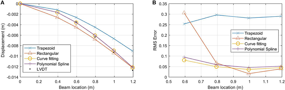
Figure 10. Cantilever beam static load tests with 16.35 N point load at the free end (A) displacement from FBG and LVDT sensors, and (B) RMS error of strain based displacement estimations at each sensor location.

Free vibration dynamic tests were also performed for the cantilever beam. The beam was displaced at the free end and released to induce a free vibration response. These tests were repeated a total of 10 times, measuring the strain and displacement response for each test. From the strain response, the displacement was calculated at each sensor location. An example of the displacement at the free end of the beam for one test is shown in Figure 11A. The RMS errors and Pearson coefficient were found for each method, see Figures 11B,C. Similar to the static analysis, the trapezoid method has the highest level of error, with a maximum RMS >27% compared to the experimental results for the simply supported boundary condition that had a maximum error of 6.5%. The error values for the other displacement estimation methods are much lower with maximum errors of 10.5% For all of the displacement calculation methods, the RMS error decreases as the location along the beam increases. However, at sensor location S5, at x = 1.2 m, the Pearson correlation coefficient decreases.

FIGURE 11

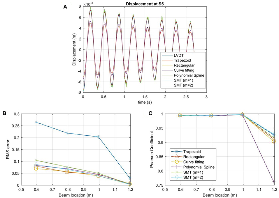
Figure 11. Experimental free vibration tests on a cantilever beam, (A) displacement at sensor location S5 (1.2 meters), (B) RMS error, and (C) Pearson coefficient.

When the laboratory tests are compared with the numerical analysis, the RMS errors are all higher in the laboratory tests due to experimental variability. Additionally, for the laboratory tests, the RMS errors for all methods have the same order of magnitude, unlike the numerical results where there was a significant difference in the order of magnitude of the error for the static analysis. For the simply supported beam static lab tests, the rectangular method performs better than expected with the lowest error in the mid-span and the trapezoid method having the highest error compared to the numerical analysis. For the simply supported beam free vibration lab tests, the results are more consistent with the numerical results except for the trapezoid method which has the highest error. For the random impact dynamic tests, the highest error is observed at the edge of the beam, which is consistent with the numerical results. For the cantilever beam static tests both the numerical and lab tests resulted in the trapezoid and rectangular methods having the highest errors with the trapezoid under estimating the displacement and the rectangular method over estimating the displacement. For the dynamic cantilever tests, the trapezoid method has a significantly higher RMS error for the lab tests whereas the rectangular method has a significantly higher RMS error for the numerical analysis. For some of the laboratory tests, there were unexpected results for the performance of the methods compared with the numerical analysis results. One factor that may account for the difference in performance is the error in the LVDT displacement measurements which is not accounted for in this analysis.

5. Application to Highway Overpass

Once assessed by numerical and experimental analysis, the strain to displacement transformation methods presented in the previous sections were also applied to data from an existing, in-service highway overpass.

5.1. Overview of Structure

The bridge is a typical highway overpass is located in the United States. The typical design is useful as it allows for the testing of SHM methods that will be widely applicable to many structures.

The structure contains multiple spans and consist of built-up steel girders of varying sizes and concrete deck, as shown in Figure 12A. The structure is skewed at the north end, providing a unique structural behavior as all girders differ in length. In this research, only the southbound span of the structure was instrumented. Two of the eight girders on the span, girder 2 and girder 5, were instrumented with sensors. On both girders, FBG strain sensors were installed in three locations: the mid span and quarter spans. These locations are shown in Figure 12B. The sensors are not evenly spaced on the structure and the total length of the two girders differ. At each location, strain sensors were installed in parallel topology on the top flange and the bottom flange for a total of 6 sensors on each girder. Additionally, a temperature sensor was installed with each strain sensor.

FIGURE 12

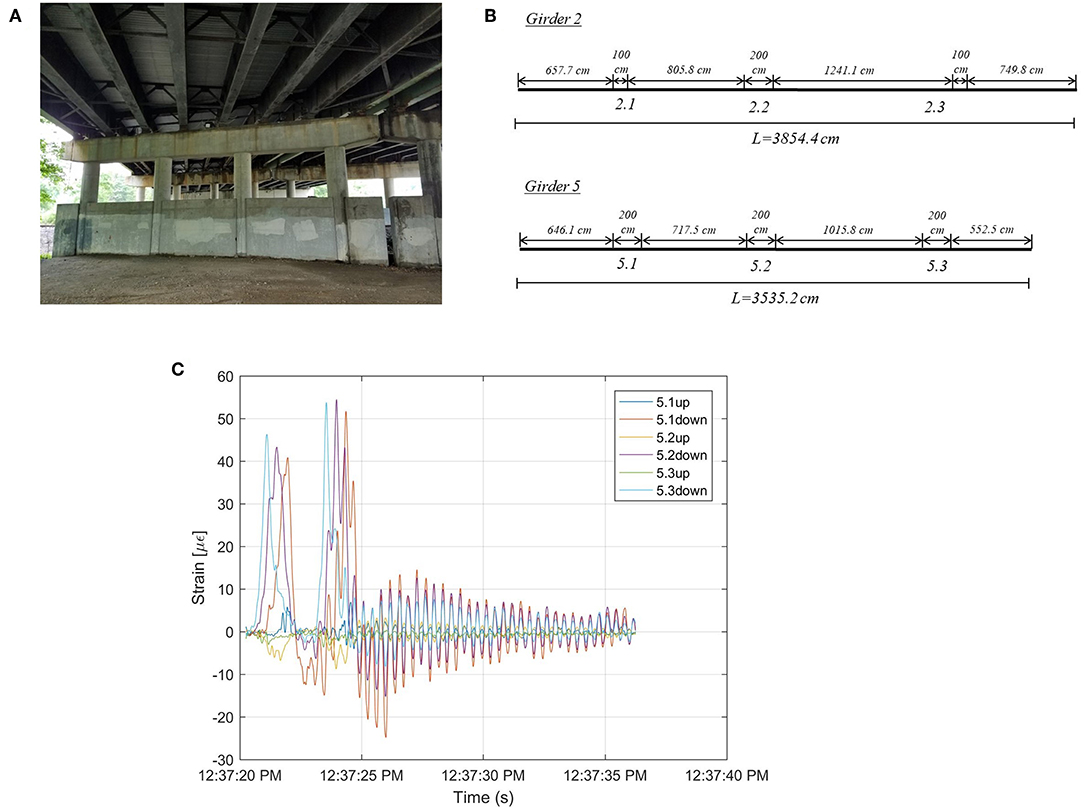
Figure 12. (A) Underside of instrumented highway overpass, (B) the sensor locations and gage lengths for girder 2 and girder 5 on the structure, and (C) typical girder 5 strain response for the structure.

Since the installment of the monitoring system on the structure periodic data collection site visits to the structure were carried out, which occurred several times throughout the year and have been ongoing for almost 6 years. During the data collection site visits, the structure remains in-service during data collection and the measurements consist of the strain response of the structure caused by the traffic loading. A total of 28 measurement session have occurred from June 2011 to January 2017. The strain response of the structure is recorded for ~1 h for each site visit and the data is recorded with a sampling rate of 250 Hz. The typical strain response for girder 5 of the structure is shown in Figure 12C, similar strain responses are observed in girder 2 however the strain amplitudes are lower as the girder is located near the edge of the structure with less traffic loading. The strain response from the sensors is filtered using a Butterworth low pass filter (Winder, 2002). The figure shows several peak strain responses on the structure followed by periods of free vibration which are the result of heavy weight vehicles passing over the structure.

5.2. Results

For all data measurement periods, the displacement of both girder 2 and girder 5 were estimated from the strain response data. The strain displacement estimation methods presented earlier in the paper were used including numerical integration (Trapezoid and rectangular methods), curve fitting, polynomial spline and SMT (m = 1 and m = 3). The displacement estimation results for one segment of monitoring the bridge with service traffic loads are shown in Figure 13 for all measurement locations on the bridge. The displacement estimation for girder 5 are higher than the displacement estimation for girder 2 because girder 5 is located in the middle of the span, more directly under the traffic lanes whereas girder 2 is located toward the edge of the structure, in line with the highway shoulder, so the traffic loading is lower. It was observed that the rectangular method estimated the highest displacements for the first quarter-span and mid-span locations on the bridge for both girder 2 and girder 5. These observations are consistent with the results observed in the experimental tests with the rectangular method typically overestimating and providing the highest displacement values and the trapezoid method underestimating and providing lower displacement values. The other methods vary in the displacement estimation but provide displacement estimation between the trapezoid and rectangular methods.

FIGURE 13

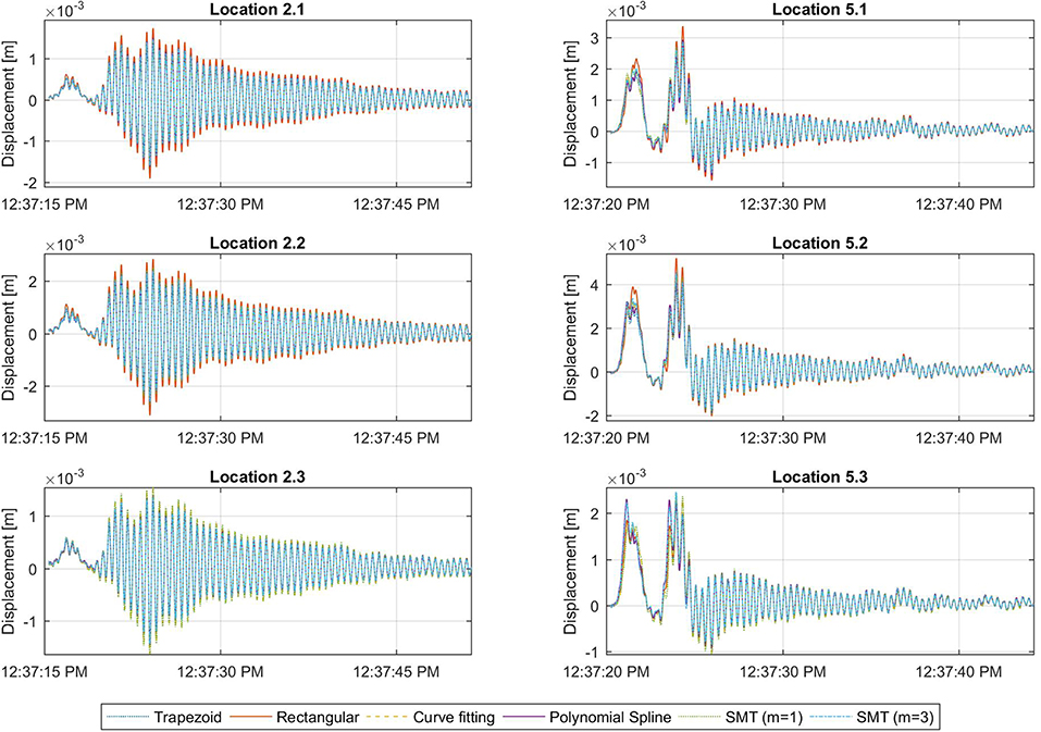
Figure 13. Displacement estimation at girders 2 and 5 from strain response due to service loads on the bridge.

5.3. Serviceability Deflection Limits

The American Association of State Highway and Transportation Officials (AASHTO) mandates that bridges without pedestrian loads have a service limit of L/800 for the live load deflections (American Association of State Highway and Transportation Officials, 2010). For girder 2 the maximum allowable deflection is 0.048 meters and for girder 5 the maximum allowable deflection is 0.044 meters. Using the deflections that were obtained from the strain measurements for both girders, a check can be performed to determine if the service limit is exceeded. For each data collection site visit the maximum deflection at each sensor location for both girder 2 and girder 5 was determined using the strain to displacement estimation methods, as shown in Figure 14.

FIGURE 14

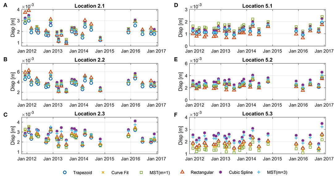
Figure 14. The maximum displacements for each sensor location on girder 2 at the quarterspans (A,C) and midspan (B) and on girder 5 at the quarterspans (D,F) and the midspan (E).

Due to the sparse sensor layout on the structure, with only three locations on each beam, variance of the different strain to displacement estimation methods is high. However, for all measurement locations on both girders, the estimated maximum deflections due to live load are significantly below the service limit for all of the estimation methods. The deflections calculated for girder 2 are slightly higher than the values found for girder 5. Additionally, as expected, the measurement location near the center of the girder had the highest deflections for both girders. Figure 14 also shows that over time, the maximum deflection values for the bridge stay relatively constant with no significant changes for all of the measurement locations.

6. Conclusions

This paper presents an evaluation and comparison of five strain-based displacement estimation methods using FBG strain sensors. These methods were successfully evaluated through static and dynamic analytical and numerical modeling and through small scale laboratory tests with a variety of loading conditions and both simply supported and cantilevered boundary conditions. The errors of the methods were evaluated to provide a comparison of the strain based methods for each scenario. The quality of estimation of displacement for each method depends on number of sensors, their location on the structure, load case, and boundary conditions of the beam. For most cases, the results show good agreement between the directly measured displacement and the estimated displacement from the strain sensors. However, the difference in estimation can be important, depending of specific application. For example, in Figure 14F, the spread of values is between 2 and 3.5 mm for various methods, which is 75% difference between the one that estimates 2 mm an the other that estimates 3.5 mm. This difference can lead to significant errors in evaluating structural health and performance of specific project (which was fortunately not the case in this specific project, please see text below). Similar considerations apply for several other evaluations shown presented in this paper. While the rectangular and trapezoid methods frequently resulted in higher errors for both the numerical and laboratory tests they require no assumptions of the curvature distribution for the beam. For many cases, the polynomial spline method can improve upon the displacement estimation compared with the rectangular and trapezoid methods and also does not require assumptions regarding the curvature distribution for the structure. However, the numerical results showed when the beam has a broken-linear curvature distribution, depending on the sensor distribution, some cases result in higher errors. Both the curve fitting and SMT methods require some assumptions regarding the curvature distribution of the beam, however they consistently had lower errors for both the experimental and numerical analysis. The methods were also applied to a real structure, a highway overpass instrumented with FBG strain sensors. It was found that all displacement during the monitoring period for the highway overpass were well below the maximum AASHTO displacement limits for all methods. This application demonstrates the potential to use the strain-based displacement methods for the monitoring of displacement service limits on a bridge.

Data Availability Statement

The datasets generated for this study are available on request to the corresponding author.

Author Contributions

KK had substantial contributions to the creation of methods and analysis and interpretation of data and drafted the paper. BG advised and supervised the work, revised the draft of the paper, and approved the final version to be submitted. Both authors are accountable for all aspects of the work.

Funding

This material was based upon work supported by NSF GRFP Grant No. 1148900, NSF CMMI-1362723, and USDOT-RITA DTRT12-G-UTC16. Any opinions, findings, and conclusions or recommendations expressed herein are those of the authors and do not necessarily reflect the views of the funding agencies.

Conflict of Interest

The authors declare that the research was conducted in the absence of any commercial or financial relationships that could be construed as a potential conflict of interest.

Acknowledgments

The authors would like to thank the following individuals for their assistance with this research: Dorotea Sigurdardottir, Dennis Smith, and Joe Vocaturo. The project on the highway overpass has been realized with the important support, great help and kind collaboration of several professionals and companies. We would like to thank SMARTEC SA, Switzerland; Drexel University, in particular Professor Emin Aktan, Professor Frank Moon (now at Rutgers University), and graduate student Jeff Weidner (now Assistant Professor at University of Texas, El Paso); New Jersey Department of Transportation (NJDOT), and in particular Nat Kasbekar and Eddy Germain; Long-Term Bridge Performance (LTBP) Program of Federal Highway Administration; PB Americas, Inc., Lawrenceville, NJ, in particular Mr. Michael S Morales, LTBP Site Coordinator; Rutgers University, in particular Professors Ali Maher and Nenad Gucunski; All IBS partners; and Kevin the lift operator. We would also like to thank Yao Yao who helped with the sensor installation.

References

Abdel-Jaber, H., and Glisic, B. (2014). A method for the on-site determination of prestressing forces using long-gauge fiber optic strain sensors. Smart Mater. Struct. 23:075004. doi: 10.1088/0964-1726/23/7/075004

CrossRef Full Text | Google Scholar

ACI 318R-11 (2011). Building Code Requirements for Structural Concrete (ACI 318-11) and Commentary American Concrete Institute (ACI). Farmington Hills, MI: ACI 318R-11.

Google Scholar

American Association of State Highway and Transportation Officials (2010). AASHTO LRFD Bridge Design Specifications. Washington, DC: American Association of State Highway and Transportation Officials.

Google Scholar

American Institute of Steel Construction (2011). Steel Construction Manual. Milwaukee, WI: AISC.

Google Scholar

American Society of Civil Engineers (2017). Minimum Design Loads and Associated Criteria for Buildings and Other Structures. Reston, VA: American Society of Civil Engineers.

Google Scholar

Bogert, P., Haugse, E., and Gehrki, R. (2003). “Structural shape identification from experimental strains using a modal transformation technique,” in 44th AIAA/ASME/ASCE/AHS/ASC Structures, Structural Dynamics, and Materials Conference (Norfolk), 1626. doi: 10.2514/6.2003-1626

CrossRef Full Text | Google Scholar

Bradie, B. (2006). A Friendly Introduction to Numerical Analysis. Upper Saddle River, NJ: Pearson Prentice Hall.

Google Scholar

Brown, C., Roberts, G., and Meng, X. (2006). “Developments in the use of gps for bridge monitoring,” in Proceedings-Institution of Civil Engineers Bridge Engineering Vol. 159, 117–119. doi: 10.1680/bren.2006.159.3.117

CrossRef Full Text | Google Scholar

Calvi, G. M., and Kingsley, G. (1995). Displacement-based seismic design of multi-degree-of-freedom bridge structures. Earthquake Eng. Struct. Dynam. 24, 1247–1266. doi: 10.1002/eqe.4290240906

CrossRef Full Text | Google Scholar

Casciati, F., and Fuggini, C. (2011). Monitoring a steel building using gps sensors. Smart Struct. Syst. 7, 349–363. doi: 10.12989/sss.2011.7.5.349

CrossRef Full Text | Google Scholar

Cigada, A., Mazzoleni, P., and Zappa, E. (2014). Vibration monitoring of multiple bridge points by means of a unique vision-based measuring system. Exp. Mech. 54, 255–271. doi: 10.1007/s11340-013-9784-8

CrossRef Full Text | Google Scholar

Corda, J., and Al-Tayie, J. (2003). Enhanced performance variable-reluctance transducer for linear-position sensing. IEE Proc. Elect. Power Appl. 150, 623–628. doi: 10.1049/ip-epa:20030563

CrossRef Full Text | Google Scholar

Davis, M., Kersey, A., Sirkis, J., and Friebele, E. (1996). Shape and vibration mode sensing using a fiber optic bragg grating array. Smart Mater. Struct. 5:759. doi: 10.1088/0964-1726/5/6/005

CrossRef Full Text | Google Scholar

Derkevorkian, A., Masri, S. F., Alvarenga, J., Boussalis, H., Bakalyar, J., and Richards, W. L. (2013). Strain-based deformation shape-estimation algorithm for control and monitoring applications. AIAA J. 51, 2231–2240. doi: 10.2514/1.J052215

CrossRef Full Text | Google Scholar

Feng, D., and Feng, M. Q. (2016). Vision-based multipoint displacement measurement for structural health monitoring. Struct. Control Health Monitor. 23, 876–890. doi: 10.1002/stc.1819

CrossRef Full Text | Google Scholar

Feng, D., and Feng, M. Q. (2018). Computer vision for shm of civil infrastructure: From dynamic response measurement to damage detection–a review. Eng. Struct. 156, 105–117. doi: 10.1016/j.engstruct.2017.11.018

CrossRef Full Text | Google Scholar

Feng, D., Feng, M. Q., Ozer, E., and Fukuda, Y. (2015). A vision-based sensor for noncontact structural displacement measurement. Sensors 15, 16557–16575. doi: 10.3390/s150716557

PubMed Abstract | CrossRef Full Text | Google Scholar

Foss, G., and Haugse, E. (1995). “Using modal test results to develop strain to displacement transformations,” in Proceedings-SPIE The International Society for Optical Engineering (Nashville, TN: Spie International Society for Optical), 112–112.

Google Scholar

Gentile, C., and Bernardini, G. (2008). Output-only modal identification of a reinforced concrete bridge from radar-based measurements. Ndt E Int. 41, 544–553. doi: 10.1016/j.ndteint.2008.04.005

CrossRef Full Text | Google Scholar

Gere, J., and Goodno, B. (2008). Mechanics of Materials. London: Cengage Learning.

Google Scholar

Glisic, B., and Inaudi, D. (2008). Fibre Optic Methods for Structural Health Monitoring. Chichester: John Wiley & Sons.

Google Scholar

Hou, X., Yang, X., and Huang, Q. (2005). Using inclinometers to measure bridge deflection. J. Bridge Eng. 10, 564–569. doi: 10.1061/(ASCE)1084-0702(2005)10:5(564)

CrossRef Full Text | Google Scholar

Jáuregui, D. V., White, K. R., Woodward, C. B., and Leitch, K. R. (2003). Noncontact photogrammetric measurement of vertical bridge deflection. J. Bridge Eng. 8, 212–222. doi: 10.1061/(ASCE)1084-0702(2003)8:4(212)

CrossRef Full Text | Google Scholar

Kang, L.-H., Kim, D.-K., and Han, J.-H. (2007). Estimation of dynamic structural displacements using fiber bragg grating strain sensors. J. Sound Vibrat. 305, 534–542. doi: 10.1016/j.jsv.2007.04.037

CrossRef Full Text | Google Scholar

Kim, N.-S., and Cho, N.-S. (2004). Estimating deflection of a simple beam model using fiber optic bragg-grating sensors. Exp. Mechan. 44, 433–439. doi: 10.1007/BF02428097

CrossRef Full Text | Google Scholar

Kirby, G. C. III., Lim, T. W., Weber, R., Bosse, A., Povich, C., and Fisher, S. (1997). Strain-based shape estimation algorithms for a cantilever beam. Proc. SPIE 3041, 788–798. doi: 10.1117/12.275704

CrossRef Full Text | Google Scholar

Kliewer, K., and Glisic, B. (2017). Normalized curvature ratio for damage detection in beam-like structures. Front. Built Environ. 3:50. doi: 10.3389/fbuil.2017.00050

CrossRef Full Text | Google Scholar

Lee, J. J., and Shinozuka, M. (2006). A vision-based system for remote sensing of bridge displacement. Ndt E Int. 39, 425–431. doi: 10.1016/j.ndteint.2005.12.003

CrossRef Full Text | Google Scholar

Leissa, A. W., and Qatu, M. S. (2011). Vibrations of Continuous Systems. New York, NY: McGraw-Hill.

Google Scholar

Marecos, J. (1978). The measurement of vertical displacements through water levelling method. Matériaux et Const. 11, 361–370. doi: 10.1007/BF02473877

CrossRef Full Text | Google Scholar

Merkle, W. J., and Myers, J. J. (2004). Use of the total station for load testing of retrofitted bridges with limited access. Proc. SPIE 5391, 687–694. doi: 10.1117/12.539992

CrossRef Full Text | Google Scholar

Nassif, H. H., Gindy, M., and Davis, J. (2005). Comparison of laser doppler vibrometer with contact sensors for monitoring bridge deflection and vibration. Ndt E Int. 38, 213–218. doi: 10.1016/j.ndteint.2004.06.012

CrossRef Full Text | Google Scholar

Park, H., Lee, H., Adeli, H., and Lee, I. (2007). A new approach for health monitoring of structures: terrestrial laser scanning. Comput. Aided Civil Infrastruct. Eng. 22, 19–30. doi: 10.1111/j.1467-8667.2006.00466.x

CrossRef Full Text | Google Scholar

Park, K.-T., Kim, S.-H., Park, H.-S., and Lee, K.-W. (2005). The determination of bridge displacement using measured acceleration. Eng. Struct. 27, 371–378. doi: 10.1016/j.engstruct.2004.10.013

CrossRef Full Text | Google Scholar

PEER (2013). Pacific Earthquake Engineering Research Center. Berkley, CA:PEER ground motion database. Available online at: https://ngawest2.berkeley.edu/

Google Scholar

Rapp, S., Kang, L.-H., Han, J.-H., Mueller, U. C., and Baier, H. (2009). Displacement field estimation for a two-dimensional structure using fiber bragg grating sensors. Smart Mater. Struct. 18:025006. doi: 10.1088/0964-1726/18/2/025006

CrossRef Full Text | Google Scholar

Reilly, J., and Glisic, B. (2018). Identifying time periods of minimal thermal gradient for temperature-driven structural health monitoring. Sensors 18:734. doi: 10.3390/s18030734

PubMed Abstract | CrossRef Full Text | Google Scholar

Ribeiro, D., Calçada, R., Ferreira, J., and Martins, T. (2014). Non-contact measurement of the dynamic displacement of railway bridges using an advanced video-based system. Eng. Struct. 75, 164–180. doi: 10.1016/j.engstruct.2014.04.051

CrossRef Full Text | Google Scholar

Ruiz-García, J., and Miranda, E. (2003). Inelastic displacement ratios for evaluation of existing structures. Earthquake Eng. Struct. Dynam. 32, 1237–1258. doi: 10.1002/eqe.271

CrossRef Full Text | Google Scholar

Shin, S., Lee, S.-U., Kim, Y., and Kim, N.-S. (2012). Estimation of bridge displacement responses using fbg sensors and theoretical mode shapes. Struct. Eng. Mechan. 42, 229–245. doi: 10.12989/sem.2012.42.2.229

CrossRef Full Text | Google Scholar

Sigurdardottir, D. H., and Glisic, B. (2014). Detecting minute damage in beam-like structures using the neutral axis location. Smart Mater. Struct. 23:125042. doi: 10.1088/0964-1726/23/12/125042

CrossRef Full Text | Google Scholar

Sigurdardottir, D. H., Stearns, J., and Glisic, B. (2017). Error in the determination of the deformed shape of prismatic beams using the double integration of curvature. Smart Mater. Struct. 26:075002. doi: 10.1088/1361-665X/aa73ec

CrossRef Full Text | Google Scholar

Vurpillot, S., Inaudi, D., and Scano, A. (1996). Mathematical model for the determination of the vertical displacement from internal horizontal measurements of a bridge. Proc. SPIE 2719, 46–53. doi: 10.1117/12.238852

CrossRef Full Text | Google Scholar

Wang, Z.-C., Geng, D., Ren, W.-X., and Liu, H.-T. (2014). Strain modes based dynamic displacement estimation of beam structures with strain sensors. Smart Mater. Struct. 23:125045. doi: 10.1088/0964-1726/23/12/125045

CrossRef Full Text | Google Scholar

Winder, S. (2002). Analog and Digital Filter Design. Oxford: Newnes. doi: 10.1016/B978-075067547-5/50016-6

CrossRef Full Text | Google Scholar

Xu, H., Ren, W.-X., and Wang, Z.-C. (2015). Deflection estimation of bending beam structures using fiber bragg grating strain sensors. Adv. Struct. Eng. 18, 395–403. doi: 10.1260/1369-4332.18.3.395

CrossRef Full Text | Google Scholar

Young, D., and Felgar, R. (1949). Tables of Characteristic Functions Representing Normal Modes of Vibration of a Beam. The University of Texas Publication No. 4913, Austin.

Google Scholar