Exploring the Feasibility of Using Commercially Available Vertically Pointing Wind Profiling Lidars to Acquire Thunderstorm Wind Profiles

Introduction

Knowledge of the low-level wind profile in and near thunderstorms can be useful to many aspects of both atmospheric science and wind engineering. As such, efforts to obtain field measurements of thunderstorm wind profiles have used both in situ anemometry mounted on tall towers (Goff, 1976; Wakimoto, 1982; Sherman, 1987; Lombardo et al., 2014) and remote sensing platforms, such as mobile Doppler-radars and radar profilers (Mueller and Carbone, 1987; Gunter and Schroeder, 2015), to acquire horizontal wind speed and direction profiles within thunderstorms. Where full-scale data have lacked, numerical simulations of isolated downdrafts impinging on a surface have been performed (Kim and Hangan, 2007; Mason et al., 2010; Vermeire et al., 2011; Orf et al., 2012). This body of research has highlighted many of the characteristics that differentiate thunderstorm winds from non-thunderstorm boundary layer winds, such as wind profiles that deviate from boundary layer theory, non-stationary ramps and lulls, complex turbulence characteristics, and non-zero vertical velocity components. As computational power increases and models become more and more sophisticated (e.g., Orf et al., 2012), more observations will be needed to help validate model results. Outside of fortuitous data collection, most of these observations will need to come from targeted field projects. Scanning mobile Doppler radars and radar profilers are frequently employed in severe thunderstorm field projects, but the quality and quantity of near-surface data is often limited by terrain, ground clutter, and scanning requirements in terms of scanning systems (Snyder and Bluestein, 2014). Typical profiling systems may not be subject to such issues, but radar profilers still have limited data availability near the surface and relatively poor spatial and temporal resolution.

In addition to the afore mentioned instruments, wind profiling lidars are also able to provide wind speed and direction profiles of the lower boundary layer and have been used extensively in the wind energy industry for both wind resource assessment and turbine control. Commercially available profiling lidar systems can generally be divided into two categories: pulsed systems and continuous wave (CW) systems. Pulsed systems operate similar to a radar profiler in that the pulse of energy is sent out and the radial velocity and range are determined by the backscattered energy and the time-of-flight of the energy (Courtney et al., 2008). Thus, the radial velocities for a series of range gates (or bins of data) are simultaneously determined for each scanned azimuth. However, time of flight considerations limit the lowest gate to 40 m above ground level (AGL) in the case of commercially available pulsed lidars. CW systems use a VAD (Velocity Azimuth Display; Browning and Wexler, 1968) technique to derive the wind vector at a specific height. The laser is focused at the programmed height, and multiple radial velocities estimates are generated as the prism rotates the laser 360° at the given height. The laser is then focused at each successive height until an entire wind profile is generated (Courtney et al., 2008; Peña and Hasager, 2011). Using this technique, the wind profile is not measured simultaneously, but there theoretically is no limitation to the lowest measurement level (Peña and Hasager, 2011). Current commercial CW lidars are able to collect meaningful data 10 m above the lidar. While the emphasis within the wind energy industry is typically placed on 10 min wind statistics at hub height (nominally 80 m), many profiling lidar systems can output the high-resolution data on which the 10 min data are based. These considerations, combined with the extensive validation of the technology (Courtney et al., 2008; Sjöholm et al., 2008; Wagner et al., 2009; Lang and McKeogh, 2011; Sathe et al., 2011, Branlard et al., 2013), the portability and the commercial availability of these instruments, suggest that profiling lidars could be beneficial to both the wind engineering and atmospheric science communities in investigating the near surface structure of the wind profile in and near thunderstorms. Despite the benefits of these instruments, questions regarding lidar data availability in and near thunderstorms still remain. Further, very little information is present in the literature describing the influence of falling hydrometers on lidar-derived vertical velocities (i.e., fall-speed corrections). Such data could contribute to the understanding of thunderstorm inflow environments, low-level outflow structure and even high-resolution numerical model validation.

Since such data could benefit multiple disciplines, this research seeks to explore the feasibility of using commercially available profiling lidars to obtain low-level (<150 m) wind profile information in and near thunderstorms. To explore this idea, lidar data from a wind energy developer were acquired and analyzed. These data consist of two case studies in which a high-resolution profiling lidar was operating adjacent to a tower instrumented with traditional anemometry (sonic and cup anemometers) as two thunderstorms passed over the complex. Using these data, this research will attempt to accomplish the following objectives:

1. Demonstrate the capability and limitations of a CW profiling lidar data in thunderstorms through the analysis of two case studies.

2. Compare the lidar data with limited (10 min resolution) data from traditional anemometry to explore the validity of the data.

3. Examine the low-level kinematic structure of the two thunderstorms.

Prior to a presentation of the data, an overview of the lidar testing complex and employed instrumentation developed by the wind energy company will be provided in section Instrumentation and Data. An examination of two case studies, including a comparison of available anemometer data, will follow in section Case Studies. After a presentation of the data, conclusions and recommendations for future work will be discussed in the final section.

Instrumentation and Data

The full-scale data used for this study were collected at the lidar calibration facility of a wind energy developer (One Energy) located in Northwest Ohio. The facility, dubbed the “Science Park” is composed of a surface weather station, a calibration pole, and a level concrete pad on which a lidar can be deployed. The majority of terrain in this region of Ohio is flat and generally open. Similarly, the area around the calibration complex is flat and open with the exception of a large industrial facility that is located ~200 m due west of the lidar pad. Additionally, two 80 m tall wind turbines are located within 100 m of the site at the 315 and 174° azimuths from the lidar. Given the limited amount of data used for this study, no attempt was made to filter the data by wind direction.

Calibration Pole Overview and Data

The surface weather station records wind speed and direction at 2 m using a propeller-vane anemometer with a distance constant (λ) of 2.7 m. Temperature, relative humidity and barometric pressure are also recorded. The calibration pole consists of 2 wind vanes, 2 cup anemometers, and a 3-D sonic anemometer mounted at various heights on a standard wooden 30 m utility pole. The wind vanes are mounted at 25 m AGL, while the cup anemometers are mounted at 28 m AGL. The latter have a distance constant of 2.55 m. The sonic anemometer is mounted at the top of the utility pole (30 m) to reduce wake cause by the utility pole itself. Additionally, the 30 m height of the sonic anemometer allows for direct comparison with the 29 m level of the lidar-based wind profile. Both the sonic anemometer and wind vane orientations were scrutinized by One Energy to ensure that the wind direction output was relative to north. The offsets for each anemometer, as well as the other instrument characteristics are included in Table 1. All the data from the calibration pole and the surface weather station are collected at a resolution of 0.2 Hz, averaged into 10 min blocks, and stored by the data logger. The raw 0.2 Hz data are not stored. Internal quality control processes automatically filter out the sonic data when the 10 min lidar data are unavailable due to lidar quality control. This aggressive filtering most often occurs with during times of heavy precipitation. While the 10 min resolution data are adequate (and standard) for wind energy validation and calibration research, the 10 min averaging time is not sufficient to fully characterize thunderstorm winds. Previous research has demonstrated that averaging times of <1 min are necessary to appropriately examine the turbulence characteristics of thunderstorm outflows (Holmes et al., 2008; Lombardo et al., 2014).

TABLE 1

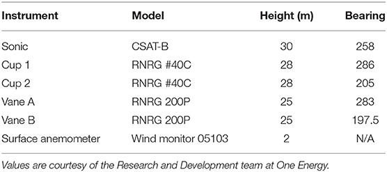
Table 1. Overview of the anemometry at the One Energy Science Park.

Lidar Overview and Data

For this dataset, a ZephIR 300 profiling lidar was placed on the lidar pad and collected data for over one year. The ZephIR 300 is a continuous wave lidar that scans conically with an offset of 30° from the vertical. This parameter, along with the distance from the unit, determines the size of probe length or the region of atmosphere that contributes to the velocity estimate at a particular level. As with Doppler radars and, to a much lesser extent, pulsed lidars, the size of range gate itself increase with distance from the unit owing to beam spread. For the ZephIR units specifically, the spatial resolution is best lower in the profile. For example, the probe length at the 10 m level is around 0.1 m (Courtney et al., 2008). As pulsed lidars maintain constant range-gate spacing with height, they are generally better above 150 m where the CW probe volume can exceed 50 m (Courtney et al., 2008; Peña and Hasager, 2011). The ZephIR units are currently capable of generating a wind profile (horizontal wind speed, wind direction, and vertical velocity) consisting of 11 different levels. For each level, 50 radial velocity samples are generated from a total of 4,000 Doppler spectra that are collected every 7.2° in azimuth (Courtney et al., 2008). The scanner takes ~1 s to perform a complete 360° rotation. Once the 50 samples have been acquired, they are plotted with respect to their azimuth, and a cosine function is fit to the data. The coefficients of the fit are then used to compute wind speed, wind direction, and vertical velocity at each height level (Courtney et al., 2008; Peña and Hasager, 2011). For the original calibration study through which the present data were collected, the ZephIR was programmed to measure at 11 heights that spanned the rotor of a standard 1.5 MW wind turbine. The programmed heights were: 29, 38, 49, 55, 59, 69, 79, 89, 99, 123, and 143 m. While the wind vector at one level only takes ~1 s to acquire, the separation time between complete wind profiles is on the order of 10s of seconds. As noted in Peña and Hasager (2011), this difference is due to the time it takes to refocus the laser, which can range from 7 to 20 s. For the two case studies examined here, the average separation between complete wind profiles was 17.1 s. The maximum time between two complete profiles was 38 s. In addition to the wind profile data collected by the lidar, a small weather station is attached to the unit. This weather station (AIRMAR 150WX) records wind speed and direction at ~1 m AGL via an ultrasonic anemometer. This unit also incorporates GPS and a compass, so that the wind directions are output relative to north. Temperature, relative humidity, and barometric pressure are also reported. The lidar weather station data are recorded at the same time as the lidar profile data and are thus available at sub-minute resolution.

The raw lidar data are recorded in a CSV file with minimal quality control. However, continuous wave lidars are prone to certain biases and data errors. For example, noise can contaminate the spectra when wind speeds are low, leading to a positive bias in wind speeds below ~4 m s⁻¹ (Peña and Hasager, 2011). Of more relevance to this study is the fact that CW lidars are not able to detect the phase of the Doppler shift, thus they cannot directly determine the sign of the radial velocity (Courtney et al., 2008; Peña and Hasager, 2011; Newman et al., 2016). If the sign of the velocity is incorrectly determined, then the wind direction will be off by 180° and the vertical velocity will have the opposite sign. To mitigate this issue, the lidar software uses the wind direction of the attached weather station to determine the “ballpark” of the wind direction and assigns to the lidar data the direction that most closely corresponds to the surface data. This assumption of a similar wind direction with height frequently breaks down in times of low wind speeds or large wind shear. The thunderstorm gust front and outflow can have both of these characteristics. As such, the 29 m lidar data used in this study were examined for 180° offsets from the 30 m sonic anemometer and wind vane direction data. Multiple instances of this error were discovered in the 48 h of data analyzed, but only one appeared to be associated with a thunderstorm outflow on 3 July 2017. As the calibration pole data (including the 2 m weather station) were only available at 10 min resolution, the 1 min National Weather Service Automated Weather Observation System (ASOS) data (available in a 2 min running average; NCDC, 2006) from the Findlay airport ~10 km to the south-southwest and the 1 m weather station attached to the lidar were used to determine the range of lidar data affected by the error. As seen in Figure 1A, both the ASOS and the lidar weather station recorded a rapid change in the wind direction associated with the outflow after 21:30 and 21:32 UTC on 3 July 2017, respectively. At this time, the unmodified 29 m lidar wind direction shows very little change in wind direction. As suggested in the literature, the lidar wind direction were corrected by adding 180° to the 2 min averaged values (Peña and Hasager, 2011). This error also effects the sign of the vertical velocity (Figure 1B; Peña and Hasager, 2011). For the same range of data points indicated in Figure 1A, the sign on the vertical velocity was switched. There is no indicator in the raw lidar data where, exactly, these errors begin. Thus, the start and end points of the corrected data are somewhat subjective in this case due to the limited resolution of the calibration data. Based on the results of 1 min resolution data analysis, all of the raw data collected on 3 July 2017 between 21:30 and 22:57 UTC were corrected.

FIGURE 1

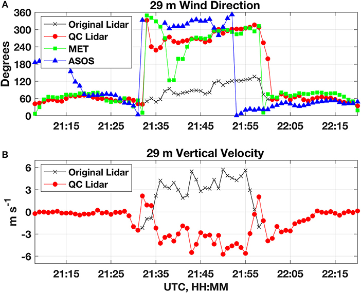
Figure 1. Comparison of (A) corrected, quality controlled (QC) lidar, ASOS, surface MET station, and non-quality controlled lidar wind direction for the 3 July 2017 dataset (B) corrected and non-corrected lidar vertical velocities from the same dataset.

Case Studies

While multiple thunderstorm events were recorded throughout the lidar deployment, two events are analyzed in this study: a single-cell thunderstorm that produced a severe wind gust on 3 July 2017 and a non-severe thunderstorm cluster on 23 July 2017.

3 July 2017

Thunderstorms initiated near a cold front that was oriented west to east across northern Indiana, Ohio, and Pennsylvania in a weakly sheared environment. These storms propagated to the east-southeast and reached the One Energy Science Park near Findlay, Ohio, around 21:30 UTC. Data from the WSR-88D in Fort Wayne, Indiana, were used not only to determine the type of thunderstorm that produced the outflow, but to also assess the radar reflectivity over the location of the lidar as it collected data during the event. These data revealed that the thunderstorm was a relatively isolated single-cell with maximum reflectivity values between 55 and 60 dBZ. As the thunderstorm passed over the location of the lidar, reflectivity values ranged from 27.5 dBZ to a maximum of 52 dBZ at 21:40 UTC and again at 21:46 UTC. However, it should be noted that these reflectivity values are from ~3.6 km AGL due to the distance between the radar and the lidar location. In addition to the heavy rain, the ASOS station located at the Findlay airport recorded a 50 knot (25.7 m s⁻¹) gust at 21:38 UTC.

Wind Time Histories

Data collected at the One Energy Science Park demonstrate a relatively typical thunderstorm outflow consisting of a rapid increase in wind speeds just after 21:30 UTC as demonstrated by the 29 m instantaneous lidar wind speeds (Figure 2A). The elevated wind speeds persisted for over 25 min, with the peak at most levels occurring between 21:50 and 21:55 UTC. At all heights measured by the lidar, the outflow was composed of multiple “pulses” of faster wind speeds separated by relative lulls. This pulsing nature has been noted in other observational and modeling studies of thunderstorm winds as well (Lombardo et al., 2014). Rapid changes in wind direction were also recorded by the lidar for this event. Prior to the passage of the gust front the winds were generally from the east-southeast. However, the wind direction was quite variable prior to the outflow owing to the lower wind speeds. Within the outflow, the wind direction veered to the west and eventually to the north before returning to an easterly direction after the passage of the outflow (Figure 2B). The vertical velocity was also recorded through the entire event and demonstrated an interesting evolution as seen in Figure 2C. Prior to the passage of the thunderstorm outflow, vertical velocities were generally weak in magnitude and variable in sign. While outflow itself was generally associated with negative vertical velocities (downdraft), there were two periods of positive vertical velocities near the beginning and the end of the event. This evolution could be related to a descending ring vortex impinging on the surface and traveling radially outward from the downdraft. Such an evolution and response are similar to those seen in numerical models (e.g., Kim and Hangan, 2007; Mason et al., 2010). An approximate size of this feature can by estimated by considering a radar-estimated storm motion of 7.7 m s⁻¹ and assuming the features of the storm are steady-state. Combining these assumptions with the difference in time between the two maxima in vertical velocity (25 min and 8 s) yields an approximate size of 11.6 km. The vertical velocities approached −7 m s⁻¹ at many of the 11 measurement heights. While this is similar to what has been documented at higher atmospheric levels in the limited previous literature (Mueller and Carbone, 1987; Sherman, 1987; Martner, 1997), the present data are likely contaminated by the speed of falling hydrometers. A similar effect is seen in radar estimations of vertical velocity. Raindrop fall speed corrections based on radar reflectivity are typically applied to radar-derived vertical velocities (Miller and Strauch, 1974), but no such correction has been developed for lidar data to the author's knowledge. Therefore, the reported vertical velocities within the thunderstorm likely contain both a component of the vertical wind and a component of the falling precipitation.

FIGURE 2

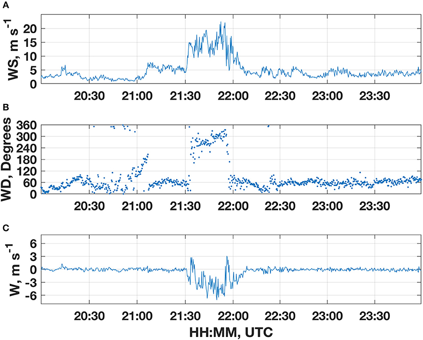
Figure 2. Time series of the 29 m (A) horizontal velocity, (B) wind direction, and (C) vertical velocity measured by the ZephIR lidar during the 3 July 2017 thunderstorm event.

Wind Profiles

The wind time histories for each level were combined at each time step to produce wind profiles from 29 to 143 m AGL. The 1 min averaged wind data were used to generate wind profiles from the 25 min prior to the outflow (the pre-storm regime) and the 25 min of outflow winds (the outflow regime). The mean profile of each regime can be seen in Figures 3A,B. The 1 min averaged wind direction at 29 m was used to separate the two regimes, with the pre-storm data corresponding to a time period of faster (4–6 m s⁻¹) winds from the east and the outflow data corresponding to the time period of strong winds (>10 m s⁻¹) from the northwest (Figure 3C). The pre-storm profile in Figure 3A is similar to what may be described by Monin-Obukhov similarity theory and the appropriate stability assumption (Foken, 2006). The profile from the outflow regime is quite different with the greatest 1 min averaged wind speeds found in the lowest two levels. To further examine the outflow profiles, individual 1 min averaged wind speed and vertical velocity profiles were selected and plotted in the context of the 29 m wind speed time history. A sample of the 1 min outflow profiles is included in Figure 4. These profiles also include the 1 min averaged wind speeds from the weather station attached to the lidar for reference. At the onset of the thunderstorm winds, the horizontal wind speed profile is similar to those seen in numerical models of impinging jets with the fastest wind speeds between 50 and 100 m AGL (the black profile in Figure 4A). The vertical velocity profile for this time step (black profile in Figure 4B) is entirely negative, indicating that downdrafts were the predominate vertical motion. 25 min later, the wind speed maximum decreased in altitude to between the 30 and 50 m levels, but it also increased in magnitude with a maximum of 18.6 m s⁻¹ at the 55 m level (blue profile in Figure 4A). The vertical velocities for this time period were also more negative with a value of −5.6 m s⁻¹ at the 29 m level (blue profile in Figure 4B). Interestingly, the vertical velocity profile also displays the greatest (negative) wind speeds in the lowest 20 m of the profile.

FIGURE 3

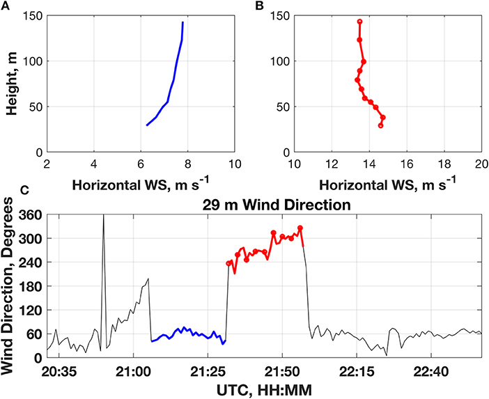
Figure 3. Estimation of average inflow and outflow wind profiles for the 3 July 2017 thunderstorm event. (A) shows the average inflow profiles (blue) based on the blue highlighted region of the 29 m wind direction in (C). (B) Shows the average outflow wind profiles (red) from the red highlighted region of the 29 m wind direction time history in (C).

FIGURE 4

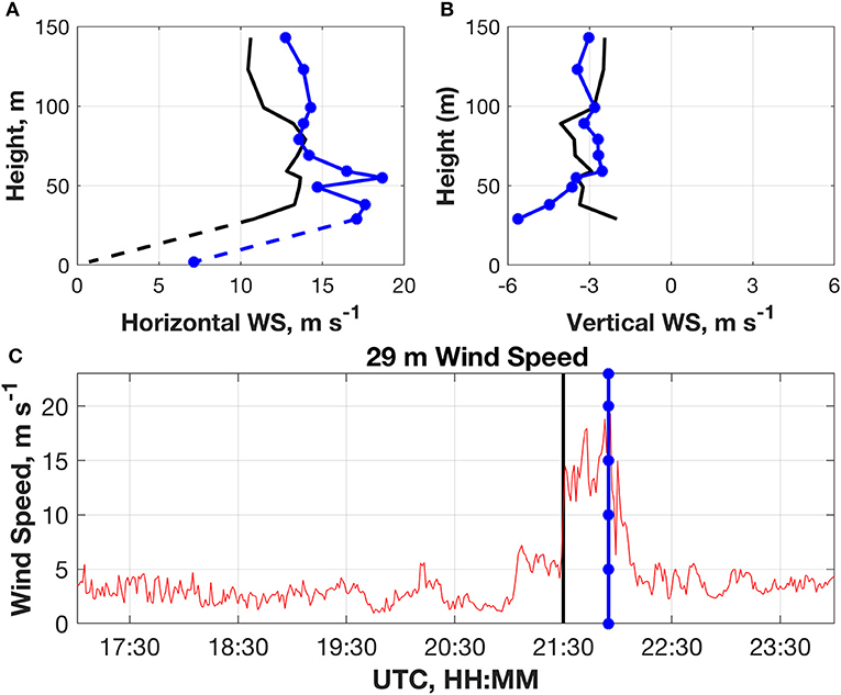
Figure 4. Comparison of the 1 min averaged (A) horizontal velocity profiles and (B) vertical velocity profiles at two different times (C) from the 3 July 2017 thunderstorm event. The profiles from earlier in the outflow are drawn in black, while the profiles from later in the outflow are drawn in blue.

Comparison With in situ Anemometry

To examine the validity of the lidar data, comparisons of the 10 min lidar wind speeds and 10 min calibration pole data were performed. Unfortunately, the data logging software filtered out the sonic data during the thunderstorm. As such, comparisons of sonic data were not available during the thunderstorm outflow for this case, but cup anemometer and wind vane data were available for horizontal wind speed and direction comparisons. As seen in Figure 5, there were very few differences between the 10 min average wind speeds recorded by the three measurement platforms throughout the day. Within the thunderstorm outflow, the lidar reported a higher peak 10 min wind speed at 29 m than the cup anemometer at 28 m. The values were 14.8 and 11.7 m s⁻¹, respectively. Considering the entire 24 h time period, the means of the three measurement devices (cup1, sonic, and 29 m lidar) differed by <0.5 m s⁻¹. Also included in Figure 5 are the standard deviation values of each 10 min period for the three measurement platforms. As expected, the standard deviation values associated with the sonic anemometer data (where reported) were higher than those of either the lidar or the cup anemometer (Wagner et al., 2009). The 10 min standard deviations for the 29 m lidar data and the cup anemometer were similar in magnitude with average values of 0.51 and 0.68 m s⁻¹, respectively. Considering the available data of the sonic anemometer, the average standard deviation was 0.96 m s⁻¹. The comparison between the cup anemometer and the lidar standard deviations suggests that the limited turbulence resolved by the lidar due to the volumetric averaging may be similar to the mechanical filtering associated with cup anemometers.

FIGURE 5

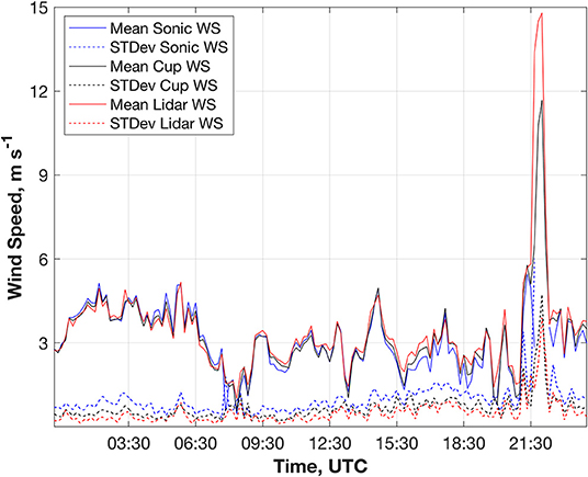
Figure 5. Comparison of the 10 min averaged horizontal wind speeds and 10 min standard deviations of the horizontal wind speeds of the different measurement platforms at the One Energy calibration complex on 3 July 2017.

23 July 2017

In a similar setup as on 3 July 2017, a broken line of thunderstorms formed along a weak cold front and propagated to the southeast. Data from the Fort Wayne, Indiana, WSR-88D radar indicated this line reached the lidar calibration complex around 22:20 UTC on 23 July 2017. Interestingly, the radar reflectivity values at the location of the lidar were much lower for this event than the 3 July 2017 thunderstorm. As the line approached, the principle cell in the portion of line targeting Findlay began to decrease in intensity and dissipated just west of the Science Park. As such, reflectivity values were <30 dBZ for the entire event. Very few storm reports were associated with this convective line, indicating that most of the cells were below severe criteria for wind and hail (26 m s⁻¹ and 1-inch diameter, respectively). The maximum wind gust recorded by the ASOS station at the Findlay Airport was <13 m s⁻¹.

Wind Time Histories

Despite the dissipating nature of the convection, the lidar at the Science Park reported maximum instantaneous gusts between 17 and 20 m s⁻¹ at all levels. The wind speed time series recorded by the 29 m scan of the lidar is presented in Figure 6A. These data show a very well-defined peak associated with the thunderstorm outflow, followed by a more gradual decrease in the wind speed as the thunderstorm moved to the southeast. This observation contrasts with the 3 July 2017 case where the wind speeds remained elevated for a time, before decreasing rapidly. As with the 3 July 2017 case, the pulsed nature of the thunderstorm winds is evident. Coincident with the increase in wind speed, the wind direction initially veered slightly from 300 to 350° and continued to veer to the north-northeast (Figure 6B). The vertical velocities associated with outflow were mostly negative as may be expected. However, there were several periods of increasing (becoming more positive) vertical velocities embedded within the outflow (Figure 6C). Additionally, the more substantial negative vertical velocities at the 29 m level appear well after the peak in the horizontal wind speed. These greater downdraft speeds were also associated with slower horizontal wind speeds.

FIGURE 6

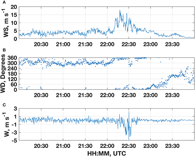
Figure 6. Time series of the 29 m (A) horizontal velocity (B) wind direction and (C) vertical velocity measured by the ZephIR lidar during the 23 July 2017 thunderstorm event.

Wind Profiles

An attempt was made to distinguish outflow wind profiles from pre-storm wind profiles as was done with the 3 July 2017 event. However, the separation between the pre-storm environment and the outflow was much more nebulous with this event. Thus, only the 1 min profiles clearly within the outflow were analyzed in Figure 7. The first horizontal wind speed profile, taken shortly after the initial increase in wind speed associated with the outflow, was approximately linear with the profile maximum at the 143 m level (Figure 7A). The associated vertical velocity profile (Figure 7B) indicated weak downdrafts with little vertical variation in the magnitude. Twelve minutes later, the lidar portion of the wind profile was inverted such that the faster wind speeds were found at the 29 and 39 m levels. The vertical velocity profile associated with this time step also indicated stronger downdrafts.

FIGURE 7

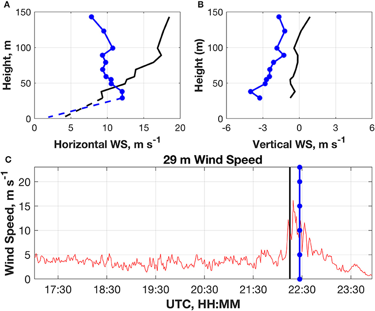
Figure 7. Comparison of the 1 min averaged (A) horizontal velocity profiles and (B) vertical velocity profiles at two different times (C) from the 23 July 2017 thunderstorm event. The profiles from earlier in the outflow are drawn in black, while the profiles from later in the outflow are drawn in blue.

Comparison With in situ Anemometry

Unlike the 3 July 2017 dataset, all of the instruments on the calibration pole collected data throughout the entire thunderstorm event. The availability of these data provides a unique opportunity to compare the low-level thunderstorm vertical velocities measured by the lidar to those measured by the sonic anemometer. However, only 10 min averages are available due to the programming of the data logger. As with the 3 July case, the 10 min average horizontal wind speeds recorded by each instrument compared very well (Figure 8). The greatest differences occurred approximately between 11:00 and 15:00 UTC where lidar recorded higher wind speeds than the other instruments. During this time period, the wind speeds were quite low (< ~2 m s⁻¹). Previous research has noted that it is common for continuous wave lidar wind speed data to have a positive bias during periods of low wind speeds due to the effects of Relative Intensity Noise (Courtney et al., 2008). For the 10 min period during which the thunderstorm occurred, the lidar recorded a peak 10 min wind speed of 11.1 m s⁻¹, while the sonic and cup anemometer measured 10.8 and 10.5 m s⁻¹, respectively. A trend in the 10 min standard deviation similar to the 3 July case was also observed in the 23 July case such that lidar and cup anemometer standard deviations were less than those reported by the sonic in each 10 min period (Figure 8). A comparison of the vertical velocities revealed very little difference between the lidar and sonic 10 min average values with a daily average for the lidar and sonic of near zero and 0.05 m s⁻¹, respectively (Figure 9). When considering the vertical velocities during the thunderstorm, it is more informative to analyze the maximum and minimum values reported by each platform. As seen in Figure 9, the lidar generally underestimated both extrema as compared to the sonic, but both the sonic and lidar measured a substantial minimum in vertical velocity near −5 m s⁻¹ associated with the thunderstorm. Interestingly, the sonic also measured a similar maximum in vertical velocity of over +6 m s⁻¹. The lidar failed to record such a maximum during this period (Figure 9). This difference is perhaps due to the contamination of the upward vertical velocity measurements by falling precipitation.

FIGURE 8

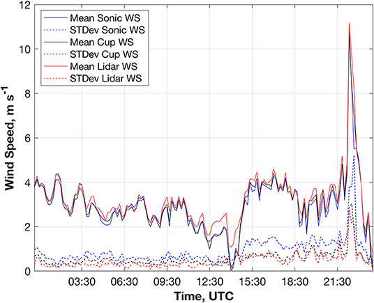
Figure 8. Comparison of the 10 min averaged horizontal wind speeds and 10 min standard deviations of the horizontal wind speeds of the different measurement platforms at the One Energy calibration complex on 23 July 2017.

FIGURE 9

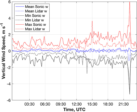
Figure 9. Comparison of the 10 min averaged, maximum, and minimum vertical wind speeds of the sonic anemometer and 29 m lidar data at the One Energy calibration complex on 23 July 2017.

Summary and Recommendations

The purpose of this study was to provide an initial look at the performance of commercially available profiling lidars in and near thunderstorms. While it is typically assumed that profiling lidars cannot provide quality data in precipitation, these examples demonstrate that the ZephIR 300 profiling lidar is able to collect reliable data during thunderstorms. Regarding the data availability and validity, the lidars were able to achieve 100% data availability throughout the two cases studied herein. It should be noted that these two cases where characterized by very different values of radar reflectivity above the location of the lidar. Much of the lidar data compared well with the existing anemometry, but substantial differences were noted between the 10 min standard deviations of the lidar and sonic data as well as the maximum (positive) vertical velocities of the two platforms. Higher resolution sonic data are necessary to more completely understand the differences in the measurement characteristics. This exploratory dataset also provided some interesting results regarding thunderstorm structure. As other studies have demonstrated, the wind profiles of these events were extremely variable during the thunderstorm outflow as well as between the events themselves. The profiles of the 3 July 2017 event often exhibited a low-level maximum around 50 m. Also, the 3 July event was much “sharper” in time with more rapid changes (ramp-ups and ramp-downs) in wind speed and direction than the 23 July event. A rare look at high-resolution thunderstorm vertical velocities also demonstrated that while downdrafts dominated most of the outflow, there were embedded periods of near zero or even positive vertical velocity. The pulsed nature of the vertical velocities is likely tied to the pulsed nature of the horizontal velocities frequently seen in thunderstorm winds, but more research is needed to verify and understand this potential connection.

While these results are promising for future work, several issues with the lidar data need to be addressed:

1. Future experiments should include disdrometer data and more detailed radar data to determine the limits of the lidar data availability in heavy precipitation.

2. Testing should be conducted to determine a consistent and repeatable method for identifying incorrect wind directions in the lidar data due to the presence of wind shear. This issue is relatively easy to identify in the 10 min data, but the greater variability of the high rate data makes determining the exact point of the error difficult.

3. An algorithm to correct the lidar-measured vertical velocity for falling precipitation should be developed. Such correction factors have been developed for vertical velocities in dual-Doppler retrievals (Miller and Strauch, 1974). These radar fall-speed corrections factors could be used to inform a lidar correction factor.

4. Examination of the scales of turbulence capable of being resolved by the lidar scanning volume. This study suggests, as others have previously (Wagner et al., 2009) the scales are similar to those resolved by a cup anemometer, but other studies suggest that CW lidars are incapable of resolving turbulence (Sathe et al., 2011; Newman et al., 2016).

Many of these issues could be addressed through a more in-depth comparison of multiple events with high-resolution sonic data at multiple levels. Despite these issues, profiling lidars have tremendous potential to collect needed data in difficult environments. The ease of deployment and narrow cone of the VAD scanning technique would support using lidars in forests to examine the impact of thunderstorm winds on trees. Alternatively, the sensitivity of these systems in clear air could allow for wind profiling in more arid regions where microbursts could be targeted. Regardless of the phenomena, lidars have the potential to contribute significantly to many of the current data needs in both atmospheric science and wind engineering.

Data Availability Statement

The datasets generated for this study are available on request to the corresponding author.

Author Contributions

Regarding the development and construction of this research article, WG was responsible for the data analysis, data interpretation, figure generation, and writing.

Conflict of Interest

The author declares that the research was conducted in the absence of any commercial or financial relationships that could be construed as a potential conflict of interest.

Acknowledgments

The author is extremely grateful to One Energy for graciously and freely providing the lidar data and the data from the calibration complex. The research and development department at One Energy was also very helpful in answering questions pertaining to the dataset. The author is also very appreciative for the comments received by three reviewers. Their comments improved both the rigor and quality of the manuscript.

References

Branlard, E., Pedersen, A. T., Mann, J., Angelou, N., Fischer, A., Mikkelsen, T., et al. (2013). Retrieving wind statistics from average spectrum of continuous-wave lidar. Atmos. Meas. Tech. 6, 1673–1683. doi: 10.5194/amt-6-1673-2013

CrossRef Full Text | Google Scholar

Browning, K. A., and Wexler, R. (1968). The determination of kinematic properties of a wind field using Doppler radar. J. Appl. Meteorol. 7, 105–113. doi: 10.1175/1520-0450(1968)007<0105:TDOKPO>2.0.CO;2

CrossRef Full Text | Google Scholar

Courtney, M., Wagner, R., and Lindelöw, P. (2008). Testing and comparison of lidars for profile and turbulence measurements in wind energy. IOP C Ser. Earth Environ. 1:012021. doi: 10.1088/1755-1315/1/1/012021

CrossRef Full Text | Google Scholar

Foken, T. (2006). 50 years of the Monin–Obukhov similarity theory. Boundary Layer Meteorol. 119, 431–447. doi: 10.1007/s10546-006-9048-6

CrossRef Full Text | Google Scholar

Goff, R. C. (1976). Vertical structure of thunderstorm outflows. Mon. Weather Rev. 104, 1429–1440. doi: 10.1175/1520-0493(1976)104<1429:VSOTO>2.0.CO;2

CrossRef Full Text | Google Scholar

Gunter, W. S., and Schroeder, J. L. (2015). High-resolution full-scale measurements of thunderstorm outflow winds. J. Wind Eng. Ind. Aerodyn. 138, 13–26. doi: 10.1016/j.jweia.2014.12.005

CrossRef Full Text | Google Scholar

Holmes, J. D., Hangan, H. M., Schroeder, J. L., Letchford, C. W., and Orwig, K. D. (2008). A forensic study of the Lubbock-Reese downdraft of 2002. Wind Struct. 11, 137–152. doi: 10.12989/was.2008.11.2.137

CrossRef Full Text | Google Scholar

Kim, J., and Hangan, H. (2007). Numerical simulations of impinging jets with application to downbursts. J. Wind Eng. Ind. Aerodyn. 95, 279–298. doi: 10.1016/j.jweia.2006.07.002

CrossRef Full Text | Google Scholar

Lang, S., and McKeogh, E. (2011). LIDAR and SODAR measurements of wind speed and direction in upland terrain for wind energy purposes. Remote Sens. 3, 1871–1901. doi: 10.3390/rs3091871

CrossRef Full Text | Google Scholar

Lombardo, F. T., Smith, D. A., Schroeder, J. L., and Mehta, K. C. (2014). Thunderstorm characteristics of importance to wind engineering. J. Wind Eng. Ind. Aerodyn. 125, 121–132. doi: 10.1016/j.jweia.2013.12.004

CrossRef Full Text | Google Scholar

Martner, B. E. (1997). Vertical velocities in a thunderstorm gust front and outflow. J. Appl. Meteorol. 36, 615–622. doi: 10.1175/1520-0450(1997)036<0615:VVIATG>2.0.CO;2

CrossRef Full Text | Google Scholar

Mason, M. S., Fletcher, D. F., and Wood, G. S. (2010). Numerical simulation of idealised three-dimensional downburst wind fields. Eng. Struct. 32, 3558–3570. doi: 10.1016/j.engstruct.2010.07.024

CrossRef Full Text | Google Scholar

Miller, L. J., and Strauch, R. G. (1974). A dual Doppler radar method for the determination of wind velocities within precipitating weather systems. Remote Sens. Environ. 3, 219–235. doi: 10.1016/0034-4257(74)90044-3

CrossRef Full Text | Google Scholar

Mueller, C. K., and Carbone, R. E. (1987). Dynamics of a thunderstorm outflow. J. Atmos. Sci. 44, 1879–1898. doi: 10.1175/1520-0469(1987)044<1879:DOATO>2.0.CO;2

CrossRef Full Text | Google Scholar

NCDC (2006). Data Documentation for Data Set 6405 (DSI-6405): ASOS Surface 1-Minute, Page 1 Data (Asheville, NC: National Climatic Data Center). Available online at: https://data.eol.ucar.edu/datafile/nph-get/353.001/td6405.pdf (accessed September 30, 2019).

Newman, J. F., Klein, P. M., Wharton, S., Sathe, A., Bonin, T. A., Chilson, P. B., et al. (2016). Evaluation of three lidar scanning strategies for turbulence measurements. Atmos. Meas. Tech. 9, 1993–2013. doi: 10.5194/amt-9-1993-2016

CrossRef Full Text | Google Scholar

Orf, L. G., Kantor, E., and Savory, E. (2012). Simulation of a downburst-producing thunderstorm using a very high-resolution three-dimensional cloud model. J. Wind Eng. Ind. Aerodyn. 104, 547–557. doi: 10.1016/j.jweia.2012.02.020

CrossRef Full Text | Google Scholar

Peña, A., and Hasager, C. B. (2011). Remote Sensing for Wind Energy. Risø National Laboratory for Sustainable Energy, Technical University of Denmark, Roskilde (Risø-I; No. 3184(EN)).

Google Scholar

Sathe, A., Mann, J., Gottschall, J., and Courtney, M. S. (2011). Can wind lidars measure turbulence? J. Atmos. Ocean Tech. 28, 853–868. doi: 10.1175/JTECH-D-10-05004.1

CrossRef Full Text | Google Scholar

Sherman, D. J. (1987). The passage of a weak thunderstorm downburst over an instrumented tower. Mon. Weather Rev. 115, 1193–1205. doi: 10.1175/1520-0493(1987)115<1193:TPOAWT>2.0.CO;2

CrossRef Full Text | Google Scholar

Sjöholm, M., Mikkelsen, T., Mann, J., Enevoldsen, K., and Courtney, M. (2008). Time series analysis of continuous-wave coherent Doppler Lidar wind measurements. IOP C Ser. Earth Environ. 1:012051. doi: 10.1088/1755-1315/1/1/012051

CrossRef Full Text | Google Scholar

Snyder, J. C., and Bluestein, H. B. (2014). Some considerations for the use of high-resolution mobile radar data in tornado intensity determination. Weather Forecasting 29, 799–827. doi: 10.1175/WAF-D-14-00026.1

CrossRef Full Text | Google Scholar

Vermeire, B. C., Orf, L. G., and Savory, E. (2011). A parametric study of downburst line near-surface outflows. J. Wind Eng. Ind. Aerodyn. 99, 226–238. doi: 10.1016/j.jweia.2011.01.019

CrossRef Full Text | Google Scholar

Wagner, R., Mikkelsen, T., and Courtney, M. (2009). “Investigation of turbulence measurements with a continuous wave, conically scanning LiDAR,” in European Wind Energy Conference and Exhibition 2009, EWEC 2009, Vol. 6 (Marseille: EWEC), 3740–3749.

Google Scholar

Wakimoto, R. M. (1982). The life cycle of thunderstorm gust fronts as viewed with Doppler radar and rawinsonde data. Mon. Weather Rev. 110, 1060–1082. doi: 10.1175/1520-0493(1982)110<1060:TLCOTG>2.0.CO;2

CrossRef Full Text | Google Scholar