Non-destructive Testing of a 100-Year-Old Reinforced Concrete Flat Slab Bridge

Introduction

The highway infrastructure is exposed to an increasing number of vehicles and heavier loads. Existing bridges often carry trucks that are significantly heavier than the original design loads. There is not enough money to strengthen or replace deficient structures. To save limited resources, there is a need for accurate evaluation of the bridges and determination of their actual resistance. Knowledge of the resistance as well as the predicted maximum expected loads, can serve as basis in important decision-making process about prioritization for repair or replacement. Therefore, the State Departments of Transportations that are responsible for maintenance of roads and bridges, can benefit from having efficient bridge evaluation procedures. The objective of the present study sponsored by the Alabama Department of Transportation (ALDOT), is to develop an approach for the evaluation of a reinforced concrete rigid frame bridge without any prior technical documentation.

Research Significance

US Bridge Inventory contains a large portion of flat slab bridges that were built in the first half of 20th century. Flat slab bridges were not designed to carry current traffic that has increased in volume and weight over the years. The bridge considered herein is an example of an old reinforced concrete flat slab structure for which there are no existing technical drawings nor other details. Currently the bridge carries unrestricted traffic, which is allowed by AASHTO’s Manual for Bridge Evaluation (AASHTO, 2011) for a reinforced concrete bridge of unknown details that has carried unrestricted traffic without developing signs of distress. Such behavior phenome is typical for this type of bridges. Research on flat slab bridges conducted up to date often involved overly conservative rating analyses based on effective width strip that in recent years were derived from FEA of slabs using shell elements.

There is no publication available that would comprehensively describe all the steps necessary to conduct non-destructive tests (NDTs) and to determine essential inputs for non-linear FE Model of a flat slab bridge. This paper illustrates how current NDT methods can be used to develop a state-of-art FE model using solid elements that can be further utilized in more accurate assessment of ultimate capacity of the flat slab bridge.

Considered Structure

The considered structure is an 11-span flat slab reinforced concrete bridge with no existing technical drawings nor other details. The bridge goes over Barnes Slough and Jenkins Creek on the northbound side of US Highway 82/231 at milepost 162.56 (Figure 1) in the State of Alabama, United States. According to archival research conducted by the research team, the bridge was constructed between 1914 and 1916, and ALDOT’s records showed that it was widened by approximately 4 ft (1.20 m) in 1930. Visual inspection of the bridge indicates that it was widened twice. It was not established when the second widenings were added.

FIGURE 1

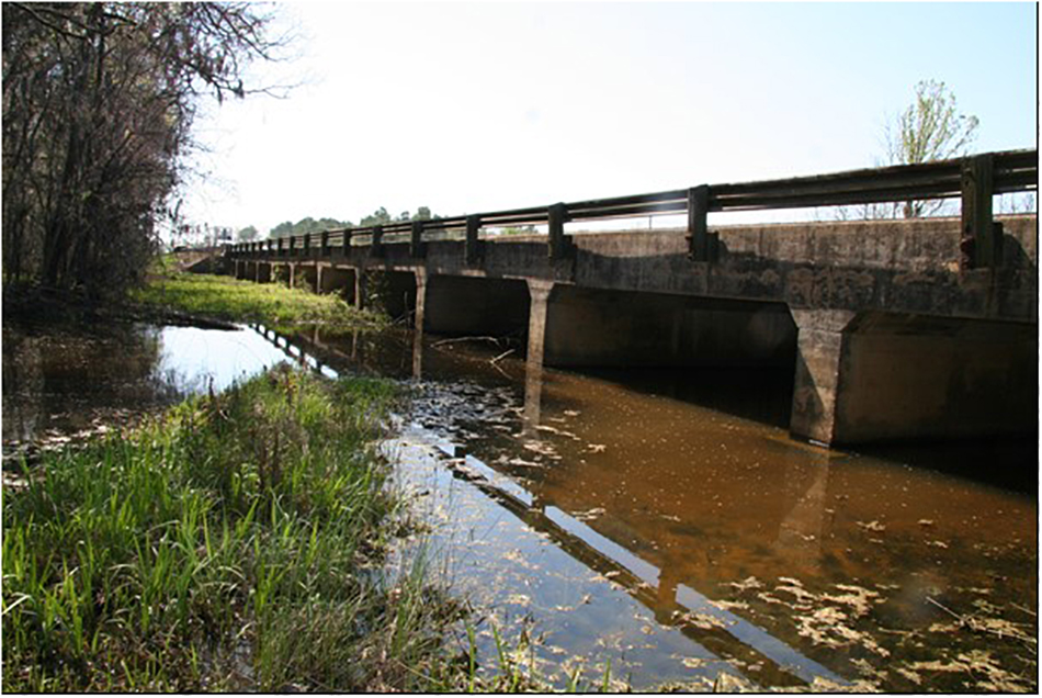
Figure 1. Side view of the bridge.

Currently ALDOT allows unrestricted traffic on the bridge based on AASHTO Manual for Bridge Evaluation (AASHTO, 2011) provisions in cases where a reinforced concrete bridge of unknown details has carried unrestricted traffic without developing signs of distress. However, because the structural details of the bridge are unknown, ALDOT cannot issue permits to overweight and non-standard trucks because this requires analytical justification.

In order to determine some of the structural parameters, the bridge was inspected and measured using field testing instruments, involving a series of destructive and non-destructive tests described in the following sections of this paper.

All 11 spans are equal, and the center-to-center span length is 21 ft – 10 inch (6.65 m), while the total width is 31 ft – 4 inch (9.53 m). Pier wall thickness is 2 ft (0.61 m). Total cross-sectional width for each span of the bridge consists of four segments: the original one and three additions. The width of the oldest segment (segment 3) is 18 ft (5.49 m). First, the bridge was widened by 3 ft – 8 inch (1.12 m) on the East side (segment 2) (Figure 2). Then it was widened on both sides by 5 ft – 4 inch (1.63 m) on the East side (segment 1) and by 4 ft – 4 inch (1.32 m) on the West side (segment 4).

FIGURE 2

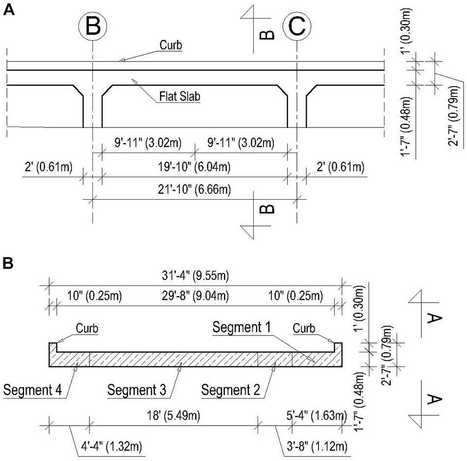
Figure 2. Detailed drawings of the bridge, (A) elevation view A-A, (B) cross-section B-B.

Field Measurements

Bridge location required the field measurements to have minimal to no impact on busy highway traffic. The measurements performed involved measurements of span dimensions, slab thickness, as well as detection and measurement of slab’s reinforcing bars. The research team used traditional tape measure, laser distance meter, a thickness measuring device, which utilizes ultrasonic pulse velocity (UPV) technology, and an advanced concrete cover meter (ACCM) that detects rebars and measures their diameters and spacings. These two high-tech instruments were operated from underneath the span and allowed to inspect the bottom reinforcement without interference with traffic. Top reinforcement was scanned with ground penetrating radar (GPR) and required lane closure. ALDOT’s qualified personnel was responsible for lane closure and top surface tests that were co-instructed by the research team. ALDOT’s certified equipment was used to obtain concrete core samples, expose bottom rebars for visual size verification, and GPR testing.

Slab Thickness

The goal in using the UPV device was to measure the thickness of concrete slab under regular traffic. Due to relatively low clearance under all the spans, ranging from about 4 to 10 ft (1.2 to 3.0 m), the measurements were taken without additional equipment required for elevated works. Multiple locations under first and second span were scanned with UPV device at original and newer widened parts of the slab. Due to the nature of the UPV technology, the measurements allowed to confirm that the concrete at all examined locations was sound with minor pulse velocity distortions near the top surface of the slab. This was an indication of roughened concrete at the interface with hot mix asphalt (HMA) Layer. Results of UPV thickness measurements showed that slab was 19 inch (48.3 cm) thick. This value was confirmed with measurements taken from bridge’s drainage holes with tape measure and later used in FE modeling.

Reinforcement

The location and size of bridge’s existing reinforcement was investigated using advanced detecting devices. Bottom surface of the bridge was scanned with ACCM, an instrument using electromagnetic pulse induction technology. The ACCM precisely detected locations of the bottom rebars, measured their diameters and cover thickness. A series of nine line-scans (Figures 3A,B) showed the same rebar distribution for all the scanned spans. A sample of the ACCM’s reading is shown in Figure 3C, where four different reinforcement distributions, corresponding to four slab segments, are clearly notable. Concrete cover of individual rebars detected is shown on vertical axis in Figure 3C. A summary of the bottom reinforcement found, is presented in Table 1.

FIGURE 3

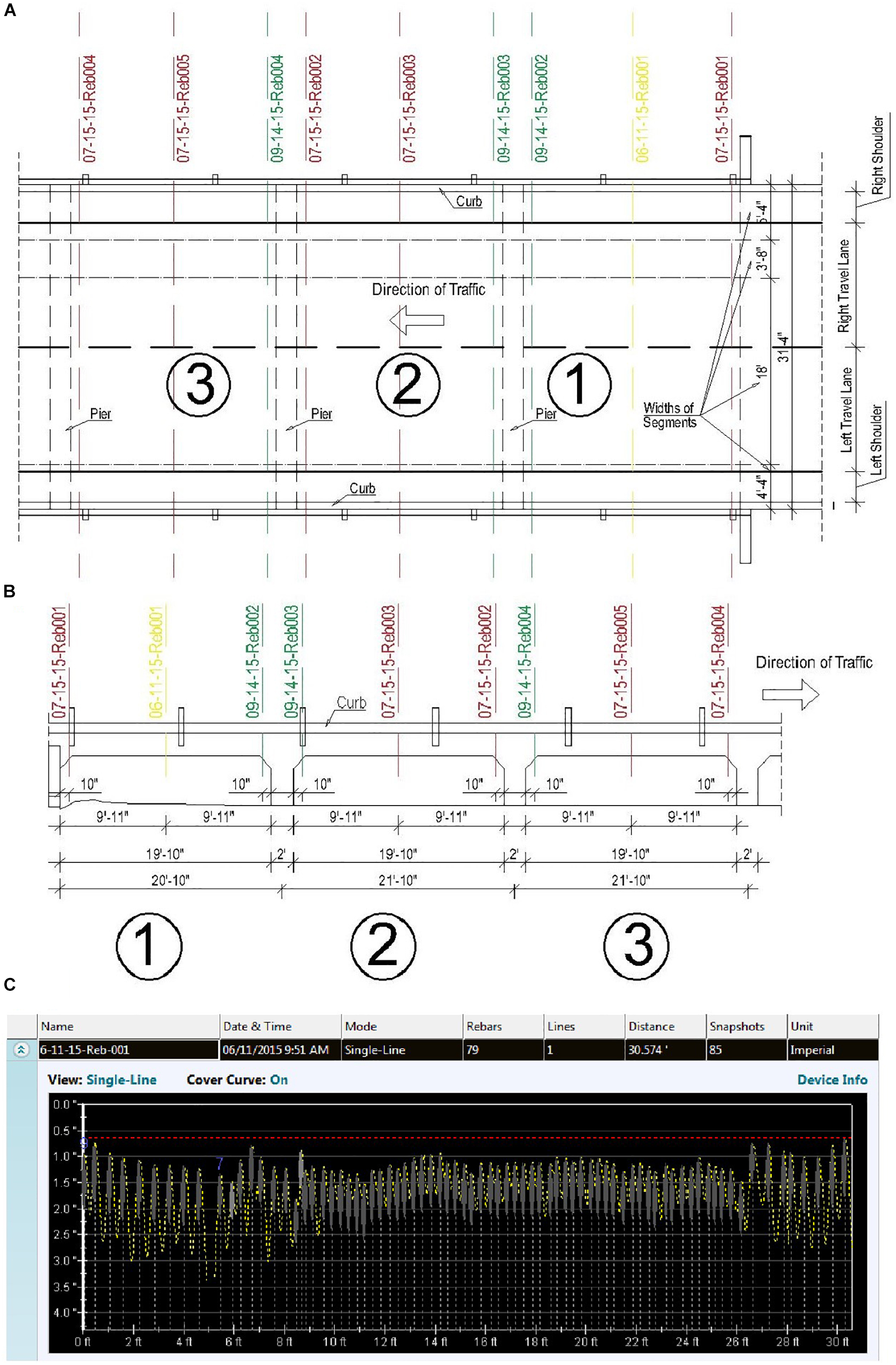
Figure 3. (A) Location of the reinforcement measurements – plan view, (B) location of the reinforcement measurements – NE elevation, (C) line measurement of reinforcing bars – scan 06-11-15-Reb001 (1 ft = 0.305 m, 1 inch = 25.4 mm).

TABLE 1

Table 1. Details of the bottom reinforcing bars.

The cover of 1.25 inch (3.2 cm) was chosen as it conservatively represents maximum clear cover read for few instances. Similar approach has driven the choice of rebars’ size, where the minimum observed diameter was selected as representative for each segment. In order to confirm ACCM’s readings the reinforcing bars were exposed in two segments. Accuracy of detecting and measuring capabilities were confirmed to be good, and interestingly, the exposed rebars turned out to be cupped. Such bar was not expected to be noticed, as around the time of bridge construction square plain bars were widely used worldwide. Additional research on old rebar types confirmed that the cupped bars were introduced to the construction industry around 1914. It was concluded that lack of bond between reinforcing bars and concrete was not an issue.

Top surface of the bridge is a 2 inch (5 cm) layer HMA, and it was investigated using the GPR. The GPR provided information on the top reinforcement distribution and detected transverse cracks in the slab over the support locations. This was also confirmed visually as presence of hair-cracks on side edges of the slab was observed. Transverse spacing of top longitudinal rebars turned out to be 12 inch (30 cm). One concrete core was drilled thru a top reinforcing bar to verify its diameter that turned out to be #4 (12 mm), as shown in Figure 4.

FIGURE 4

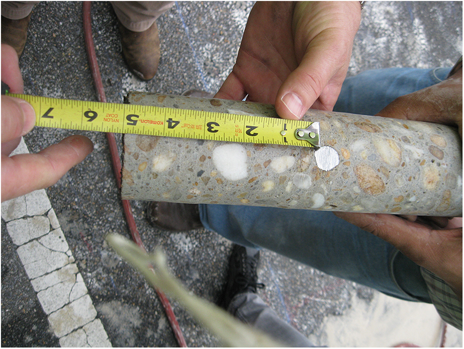
Figure 4. Cylindrical concrete sample drilled (1 inch = 25.4 mm).

All the transverse line-scan readings obtained with ACCM were thoroughly processed and analyzed, confirming that the bottom longitudinal reinforcement is extended into the supports in the three segments added to widen the bridge – Segment numbers 1, 2, and 4. For the original segment no. 3 it was found that two-thirds of the reinforcement was extended into supports and one-third was either terminated or bent up. The GPR did not detect any #8 (25 mm) or #7 (22 mm) bars at the top of the slab. Hence, it was concluded that the missing one-third of the bars were not bent up and were terminated 3.5 ft (1.06 m) from each support. Also, the core drilled from the top of the slab at the support location, showed only #4 (12 mm) rebars without any evidence of bottom bars that were bent up. With this evidence it was possible to check the development length of the one-third of the bars in the original segment. All the bottom bars were concluded to be developed based on simple span moment analysis.

Based on these findings it was concluded that the bridge was reinforced as if it is a series of simple spans, and in subsequent load capacity calculations simple support conditions were assumed with top reinforcement neglected entirely. The AASHTO Manual (AASHTO, 2011) specifies yield strength for reinforcing bars by considering the date of construction. For unknown steel constructed prior to 1954, the yield strength F_y is given as 33 ksi (227 MPa).

Concrete

At least three different concrete mixes were used in the bridge. Due to restrictions on the number of cores that could be drilled, only three concrete samples were available. One core was drilled in original segment no. 3 (Figure 2), in the oldest concrete, at over the support location. Additional two cores were taken from segment no. 1 with the newest concrete, at over support and mid-span locations. Concrete cylinder compressive strength values obtained in ALDOT’s material laboratory are presented in Table 2. For superstructure components constructed prior to 1959 AASHTO Manual (AASHTO, 2011) recommends a minimum compressive strength value of 2500 psi (17.2 MPa), which turned out to be under conservative for segment 1.

TABLE 2

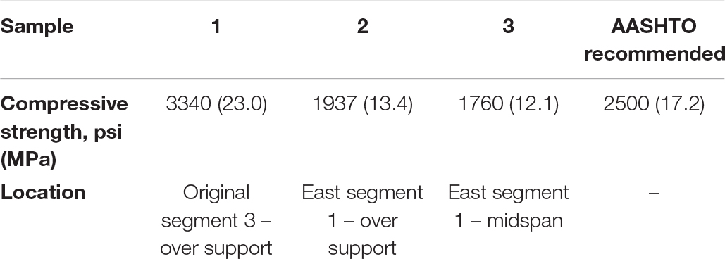
Table 2. Compressive test results for concrete cores.

Load Tests

Bridge load testing program should be planned ahead and consider individual conditions related to the structure as well as its site specifics (Amer et al., 1999; Chajes and Shenton, 2006; Sanayei et al., 2012; Davids and Tomlinson, 2016). Flat slab bridges usually are supported on maximum 15–20 ft (4.5–6.0 m) tall piers and provide enough clearance to inspect the bottom of the slab span. Investigated bridge carries traffic of a busy highway and closure of the bridge to conduct live load tests was not permitted. Instead, one lane was closed to commence the tests. Low clearance under the bridge allowed to easily instrument the bridge with sensors measuring strains and deflections.

Testing Plan

To investigate the behavior of a hybrid structure consisting of four concrete segments (Figure 2), three kinds of load tests were conducted. The first test was conducted for determining the static response under multiple load patterns. This test was performed with a truck placed on the bridge without any movement. Then, selected load patterns were repeated with the trucks moving at a crawling speed. Finally, the trucks moved over the bridge with a speed of 61 mph (98 km/h), to check the dynamic response of the bridge.

Two 85.1-kip (38.6-ton) test trucks configured according to ALDOT’s LC-5 Load Case (Figure 5A) were used as the live load and were placed on the bridge in configurations as listed below:

FIGURE 5

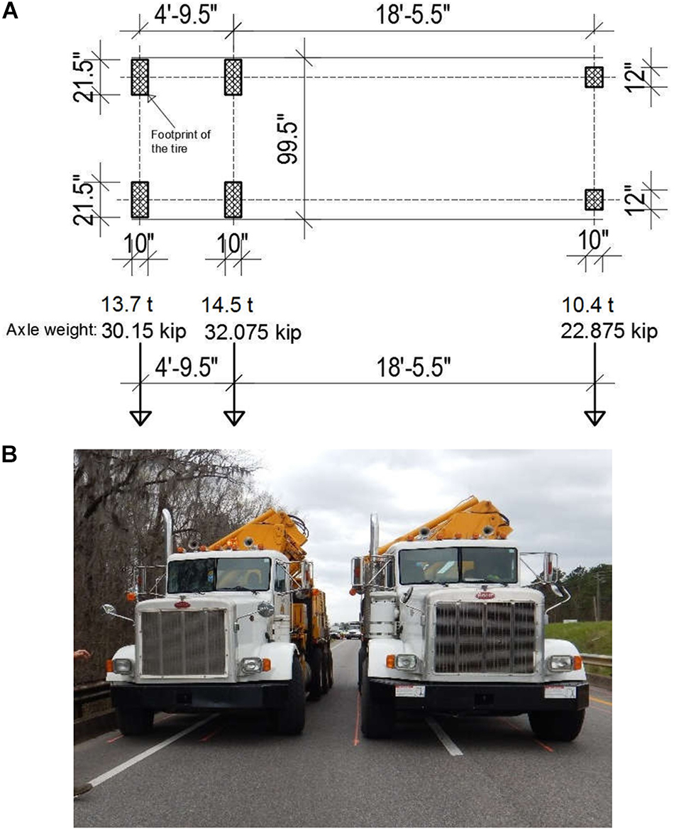
Figure 5. (A) Load configuration and axle spacing for ALDOT’s Load Case LC-5, (B) example load pattern LP-4-R.

(1) LP-1-R: Static loading. One truck placed in the middle of right traffic lane*

(2) LP-1-L: Static loading. One truck placed in the middle of left traffic lane*

(3) LP-2-R: Static loading. One truck placed 1 ft (0.3 m) from right curb*

(4) LP-2-L: Static loading. One truck placed 1 ft (0.3 m) from left curb*

(5) LP-3-R: Crawling speed. LP-1-R truck passing at crawling speed, no stops**

(6) LP-3-L: Crawling speed. LP-1-L truck passing at crawling speed, no stops**

(7) LP-4-R: Static loading. Two trucks placed side-by-side 1 ft (0.3 m) from right curb* (Figure 5B)

(8) LP-4-L: Static loading. Two trucks placed side-by-side 1 ft (0.3 m) from left curb*

(9) LP-5-R: Speed = 61 mph (98 km/h). LP-1-R truck passing at speed of 61 mph (98 km/h), no stops**

* For all static load patterns, second axle of truck/trucks located at midspan.

** Non-static load patterns are not presented in this paper due to insignificant differences with results obtained for static cases.

The trucks were placed in both lanes of the bridge to produce heavy loading in the critical locations corresponding to design by AASHTO (AASHTO, 2001).

Strains and deflections are the two most common measurements taken during live load testing of the bridges. For the flat slab bridges strains and deflections are two most effective measurements as per AASHTO Manual (AASHTO, 2011). BDI equipment was chosen for these tests because of its good reputation and performance in similar research projects.

For measurements of the strains, strain transducers (ST) with special extensions were mounted at the bottom of the slab and covered with aluminum foil to reduce “drift” effect due to the change of the temperature (BDI, 2016b). Due to small values of expected strains, the aluminum extensions for STs were used for more precise measurements. The deflections were measured with Linear Variable Differential Transformers (LVDT) (BDI, 2016a). Total of 12 STs and four LVDTs were used and installed under the bridge as shown in Figure 6. The measuring system consisted of Base Station, Access Point, Data Acquisition Nodes and Sensors. The sensors were connected with a cable to the Data Acquisition Nodes, which sent data over WiFi to the Access Point and Base Station. The data was recorded at frequency of 100 Hz and required further post-processing.

FIGURE 6

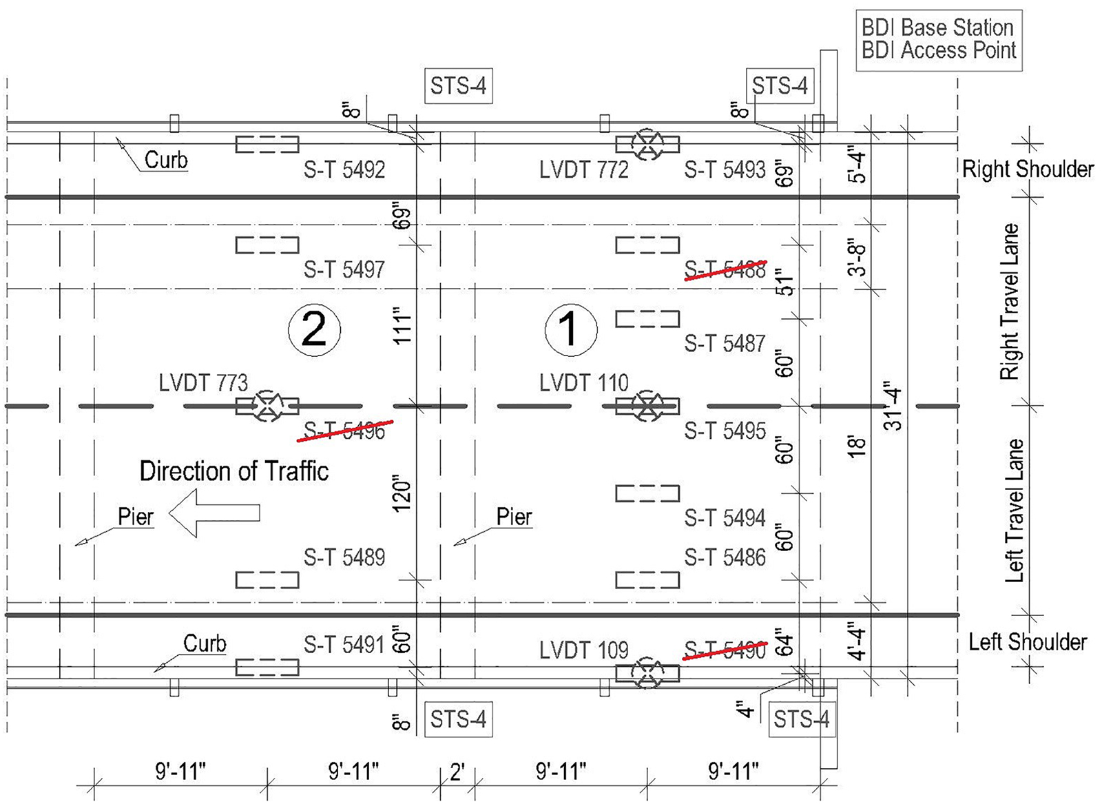
Figure 6. Strain transducers (S-T XXXX) and LVDT’s (LVDT XXX) locations.

Analysis of Field Data

Data recorded during the live load tests was further analyzed and summarized. Numerous comparisons between load cases were conducted. Transverse behavior of the bridge was verified for symmetry and consistency in measured values of strains and deflections. After the analysis of the results, data recorded by three STs (S-T 5488, S-T 5490, and S-T 5496) appeared to be incorrect and it was excluded from the database (see crossed-out sensors in the Figure 6). Since 18-inch (45.7 cm) long extensions were used with 3 inch (7.6 cm) long STs, the recorded values of strains had to be divided by 6. Manufacturer of the diagnostic system provided calibration factors for each ST as well as specified an adjustment factor of 1.1 (BDI, 2016b), which relates to aluminum extensions. These two factors were applied as multipliers to all the recoded values of strains.

For all the static load cases measured strain values from spans 1 and 2 were compared. For span 1, the pattern of strains measured in the oldest segment of the bridge is consistent with expected linear increase (Table 3). Strains measured under span 2 (Table 3) were also reasonably symmetric. This was an indication of symmetric behavior of the slab in transverse direction. The largest measured strain value was 34.3 με, recorded under span 2 for the load pattern LP-4-R being the most critical.

TABLE 3

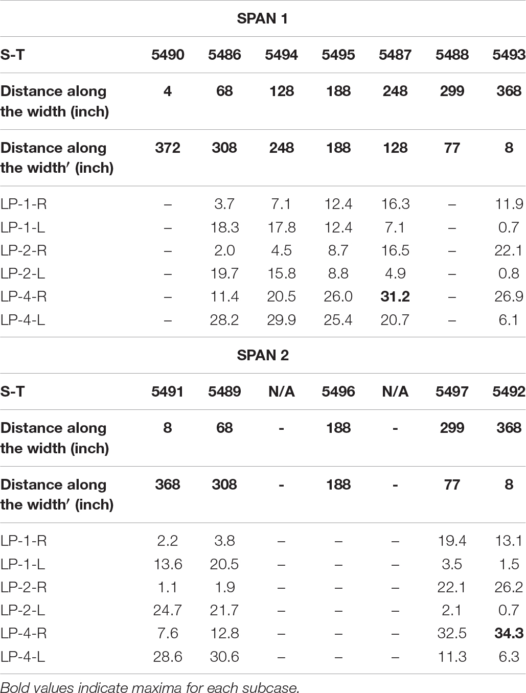
Table 3. Summary of strains for each static load pattern (με) – span 1 and 2.

Summary of the deflections recorded during load tests is shown in Table 4. Comparison of measured deflections for spans 1 and 2 at mid-width locations showed good agreement between spans, as well as reasonable symmetry for span 1. The largest deflection of 0.598 mm (0.024 inch) was recorded at the west side of span 1. This deflection was recorded under load case LP-4-L with two trucks placed side-by-side close to the curb on the west side of the bridge.

TABLE 4

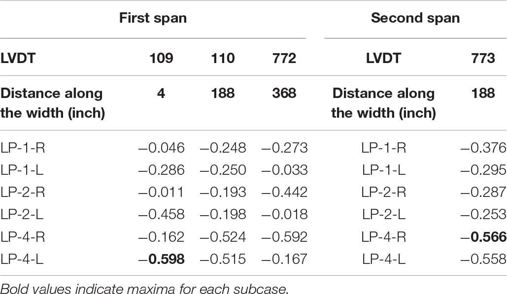
Table 4. Summary of deflections for each static load pattern (mm) (1 inch = 25.4 mm).

Finite Element Model

Bridge testing often follows a computer model development for additional analysis of the structure. Depending on the bridge type, ones’ consideration often is limited to beam-shell models for girder bridge types or shell/grillage models for flat slabs. Regardless of the modeling technique, flat slab bridges are proven to have capacities far exceeding theoretically derived values that base on flexural strength of a unit-width member (Saraf, 1998; Jáuregui et al., 2010; Davis et al., 2013). For the purpose of the research project, it was decided to develop a state-of-art FE model of the examined bridge to accurately trace stress distribution and to use it later for ultimate strength evaluation.

Based on the findings from field measurements, a FE model of a single span of the bridge (Figure 7) was developed in Simulia Abaqus FE Software. FE model was first used to predict behavior and magnitudes of stresses, strains, and deflections expected during the load tests. After the live load testing commenced the FE model was calibrated to serve as basis for further analysis.

FIGURE 7

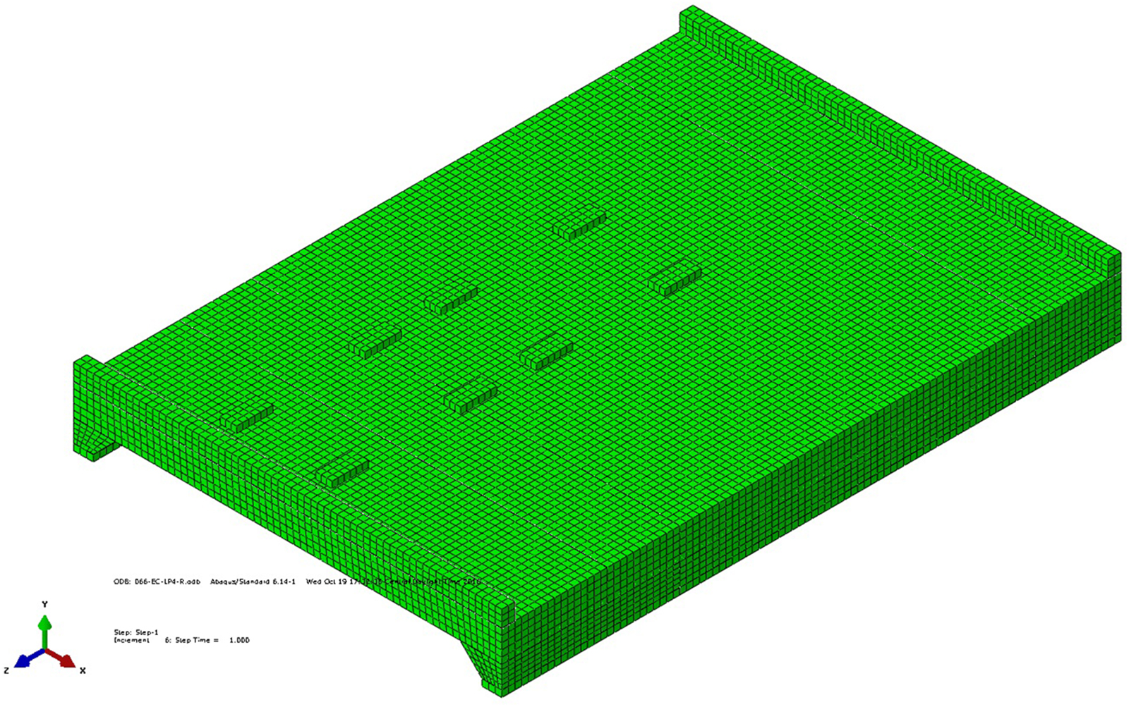
Figure 7. Isometric view of the FE Model of the Bridge. ALDOT Test Trucks footprint pattern presented.

This section presents all the input variables and their calibrated values that yielded results best matching the measured values. A three-dimensional FE model was developed with usage of solid and beam elements. The application of solid elements allowed for a detailed investigation of local stress and strain distributions as well as overall bridge behavior. The model contains upper portions of the piers, slab segments, bottom reinforcing bars, and curbs of dimensions as shown in Figure 2. The curbs have cross-sectional dimensions of 8 × 10 inch (20 cm × 25 cm). Four different width segments, fully bonded with each other, create each of the simple span slabs.

Static wheel loads on the bridge were modeled as flat rigid load transferring plates with a uniform load applied.

Element Types

Among various element types available in the finite element method (FEM) only selected elements are presented. The concrete elements – curbs, slab segments, and piers were modeled with 8-noded linear brick elements with reduced integration (C3D8R). Reduced integration element was chosen due to its computational cost, which is less than for a full-integration element. The element type used for reinforcing bars is a 2-node linear beam element (B31). The advantage of the beam over widely used link elements in FE modeling of reinforcement is its ability to act in compression as well as in tension. Both element types selected, C3D8R and B31, are suitable for stress/displacement simulations. Brick elements have three degrees of freedom active at each node – translations in the nodal x, y, and z directions. For the beam elements all six degrees of freedom (rotations and translations) at each node are computed. For this particular bridge model, the application of solid finite elements for concrete members allowed to control the contact definitions between concrete segments and resulted in more detailed investigation of localized stress and strain distributions.

The reinforcing bars were modeled as embedded into slab. From the numerical method point of view an embedded rebar acts as fully bonded with concrete slab, which was concluded from field measurements. Although, the rebars are present in all concrete members they were modeled in the slab segments only. Reinforcement in the piers was neglected due to their large dimensions and lack of detection capabilities of the sensing instrument.

One of the most important parameters that impacts accuracy of results and analysis time is FE mesh size (Logan, 2017). A mesh density study was performed by monitoring three key parameters: mesh size, convergence of results, and non-linear analysis time. This study showed that the most effective mesh size, in terms of accuracy and computing time, is 4 × 4 × 3.8 inch (10 cm × 10 cm × 9.7 cm) for the brick elements and 4 inch (10 cm) of length for the beam elements.

Numerical Material Models

In order to develop numerical material models all collected data and available literature was reviewed. FEM material models require specification of basic material parameters such as modulus of elasticity, Poisson’s ration as well as stresses with corresponding strains in inelastic stress ranges for more advanced analyses. Two non-linear material models, concrete damage plasticity (CDP) for concrete and elasto-plastic for steel, were implemented into the FE model. At the time of selection of numerical material materials benefits coming from non-linear analysis were justified by need for accurate stress investigation for loads causing concrete cracking and compressive stresses reaching their ultimate values.

Concrete Material Model

Among smeared crack and brittle crack concrete models available in Abaqus software, the CDP model was selected due to its potential to represent complete inelastic behavior of the concrete bridge elements in tension and compression and their damage characteristics. All concrete material models have their pros and cons, but for this application CDP was justified because of lack of numerical convergence issues during the analysis, overall good agreement with the test results (Chaudhari and Chakrabarti, 2012), and macro-scale of the structure for which investigation of crack development was not required. Furthermore, the CDP can be used both in Abaqus/Standard and Abaqus/Explicit, which at the time of numerical material model considerations was a valuable advantage allowing for bridge collapse simulation.

The CDP model available in Abaqus requires input of parameters associated with simplified Drucker-Prager concrete strength hypothesis. The dilation angle ψ, flow potential eccentricity ε, f_b0/f_c0 ratio (point in which the concrete undergoes failure under biaxial compression), K_c parameter (ratio of the distances between compression and tension meridians in the deviatoric cross-section) as well as Viscosity parameter describe behavior of concrete in biaxial stress state. Description and recommended values for these parameters are available in Abaqus Manual (ABAQUS, 2014) and research papers (Kamiński and Kmiecik, 2011). Plasticity parameters used were set at recommended by Abaqus Manual values: ψ = 36°, ε = 0.1, f_b0/f_c0 = 1.16, K_c = 0.667, Viscosity parameter = 0.

In addition to concrete plasticity parameters, the CDP material model definition requires stress-strain data within inelastic region for compressive and tensile behavior. These can be determined from strain-stress curve for a concrete sample. Due to lack of stress-strain data for the concrete samples taken, the relationship curves had to be developed with approximate equations.

ACI 318-14 (American Concrete Institute, 2014) provides the formula, where modulus of elasticity, E_c is a function of concrete compressive strength, f′_c.

$$E_c=57000\sqrt{f_c^{{}^{\prime }}}$$

Where:

E_c = Initial Modulus of Elasticity (output in psi),

f’_c = Compressive Strength of concrete (input in psi).

During the calibration process it was found that Eurocode formula (European Committee for Standarization, 2004) for the modulus of elasticity adopted to the FE model produces values of strains and deflections better matching the measured values. Hence, the Eurocode formula presented below was used in the material model.

$$E_c=22000{(f_c^{{}^{\prime }})}^{1/3}$$

Where E_c and f′_c in MPa.

The compressive stress-strain relationship curves were derived using Desayi and Kirshnan (1964) equation.

$${\mathrm{\sigma }}_c=\frac{E_c{\mathrm{\epsilon }}_c}{1+{\left(\frac{{\mathrm{\epsilon }}_c}{{\mathrm{\epsilon }}_0}\right)}^2}$$

Where:

σ_c = Compressive Stress,

ε_c = Compressive Strain,

ε₀ = Strain at maximum Stress,

E_c = Initial tangent modulus, assumed to be twice the secant modulus at maximum stress f′_c.

It was assumed that numerical concrete material models perform linearly up the stress of 0.4f’_c. The three presumptions on initial tangent modulus of elasticity: being a function of f’_c, being equal to twice the secant at f’_c, and it’s linearity within 0.4 f’_c allowed to derive the compressive stress-strain relationships for concrete segments based only on one input variable f’_c. Due to lack of stress-strain data from compressive tests of the samples the presented approach was considered appropriate.

The tensile stress-strain relationship was developed using the Wang and Hsu formula (Wang and Hsu, 2001), which among many other formulas is considered to most accurately describe concrete tension stiffening (Kamiński and Kmiecik, 2011).

$${\mathrm{\sigma }}_t=\{\begin{array}{c}\hfill E_c{\mathrm{\epsilon }}_t\mathit{\hspace{1em}\hspace{1em}\hspace{1em}\hspace{1em}}\mathit{if}{\mathrm{\epsilon }}_t\le {\mathrm{\epsilon }}_{\mathit{cr}}\hfill \\ \hfill f_c^{{}^{\prime }}{\left(\frac{{\mathrm{\epsilon }}_{\mathit{cr}}}{{\mathrm{\epsilon }}_t}\right)}^{0.4}\mathit{if}{\mathrm{\epsilon }}_t>{\mathrm{\epsilon }}_{\mathit{cr}}\hfill \end{array}$$

Where:

σ_t = Tensile Stress,

ε_t = Tensile Strain,

ε_cr = Cracking Strain,

In order to establish cracking strain, the modulus of rupture needs to be known. The AASHTOs’ formula (AASHTO, 2001) was used to establish the tensile strength of the concrete.

$$f_r=\{\begin{array}{c}\hfill 7.5\sqrt{f_c^{{}^{\prime }}}(\mathit{US}\mathit{units})\hfill \\ \hfill 0.623\sqrt{f_c^{{}^{\prime }}}(\mathit{SI}\mathit{units})\hfill \end{array}$$

Four different compressive strengths of concrete were taken for each of the four slab segments to develop stress-strain relationships for compressive and tensile behavior. Compressive strengths used as well as the values of corresponding moduli of elasticity are shown in Table 5. Developed curves for each of the slab’s segment are shown in Figure 8.

TABLE 5

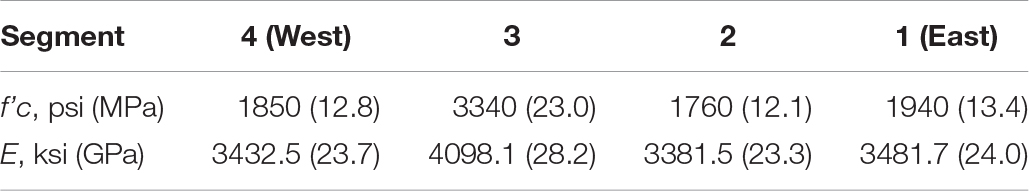
Table 5. Parameters of concrete for each of the slab’s segments.

FIGURE 8

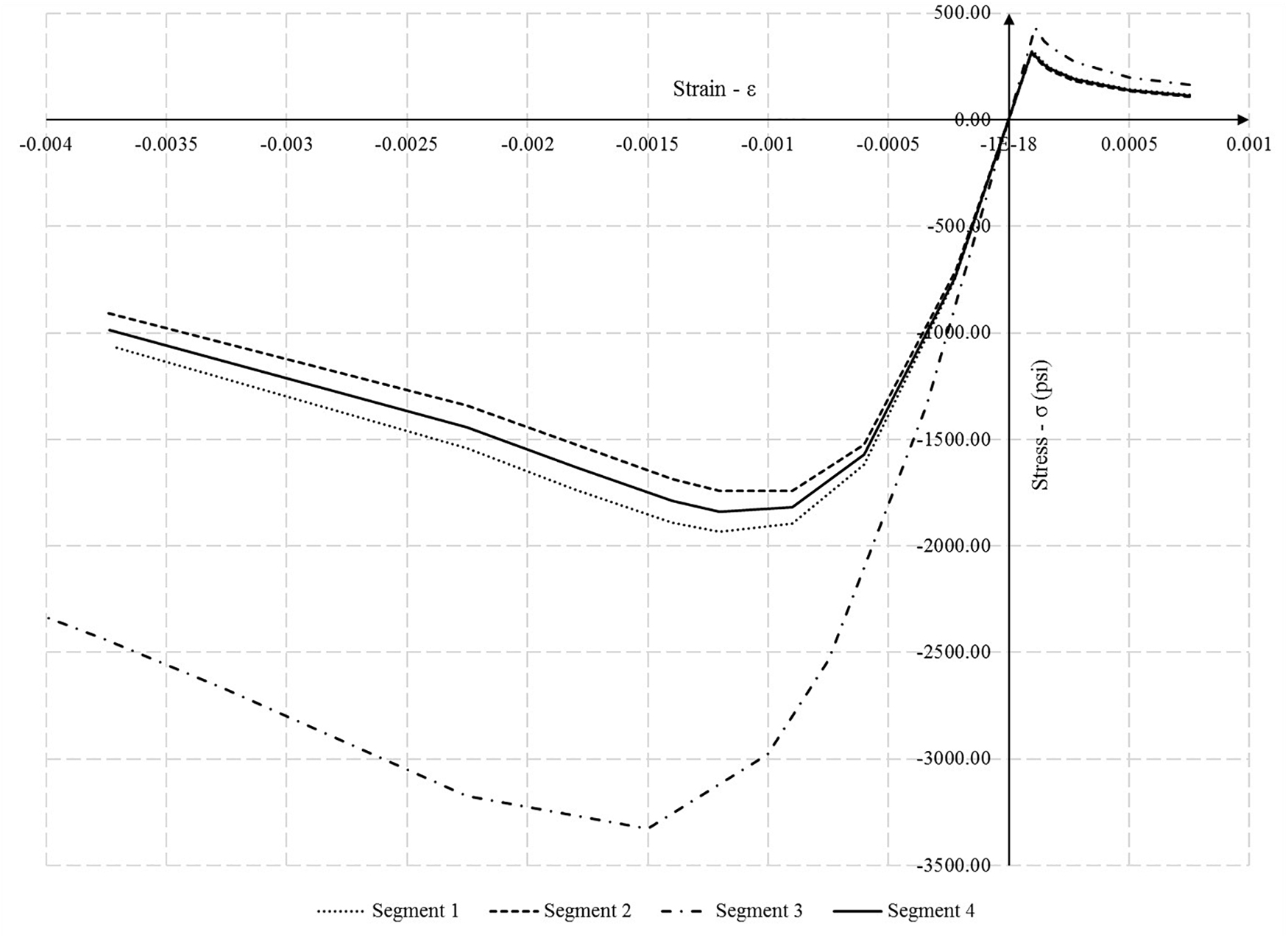
Figure 8. FEM input Stress-strain curves for segments 1–4 (100 psi = 0.69 MPa).

Steel Material Model

Provisions from AASHTO Manual (AASHTO, 2011) allowed to develop the material model for reinforcing steel bars. The Manual recommends the yield strength of steel of 33 ksi (227 MPa) for unknown reinforcing steels built prior to 1954. The ultimate tensile strength of steel was assumed to be 58 ksi (400 MPa) with slope of 2.5% of initial modulus of elasticity within inelastic region. This strain hardening of steel was input purely for numerical analysis stability purposes. The reinforcing bars reach yielding at strain value of 1.14E-3 based on assumed modulus of elasticity of 29000 ksi (200 GPa).

Boundary Conditions and Loads

The first supporting pier, at the abutment location, has restrained displacements in Y and Z directions. Unrestrained displacement in X direction allows it to move in longitudinal direction, parallel to direction of traffic. Second pier has all the displacements restrained. The rotations for both piers are allowed in all the directions.

Slab end edges were unrestrained to imitate its discontinuity due to the transverse cracks detected over the supports during the field measurements (Figure 7). Contact conditions specified in the model are as follows: full bond of reinforcing bars with concrete in all segments, full connection between side surfaces of the adjacent segments, pressure transfer interaction between tire footprint elements and concrete segments.

Load applied to the model during calibration process was the actual truck used during the live load tests. ALDOT’s LC-5 Test Truck axle spacing, footprint area, and axial loads are presented in Figure 5A.

Results

Initially developed FE model, before the load testing commenced, correctly predicted lack of concrete rupture and very small values of deflections. It was confirmed that stresses in concrete segments and reinforcing bars would remain in elastic range.

Field measured strains and deflections, for the most severe static load cases, were plotted with FEA obtained values from a calibrated model (Figures 9A,B). FEA were performed for two additional models assuming all the slab’s segments have the same compressive strength of concrete, which results in the same concrete material model throughout the slab. Plots show FEA results for the calibrated model and two models with strength of concrete of 1760 psi (12.1 MPa) and 3340 psi (23.0 MPa). Values on the horizontal axis correspond to the total width of the bridge and limits of adjacent segments (Figure 2B) are indicated with vertical dash-dotted lines.

FIGURE 9

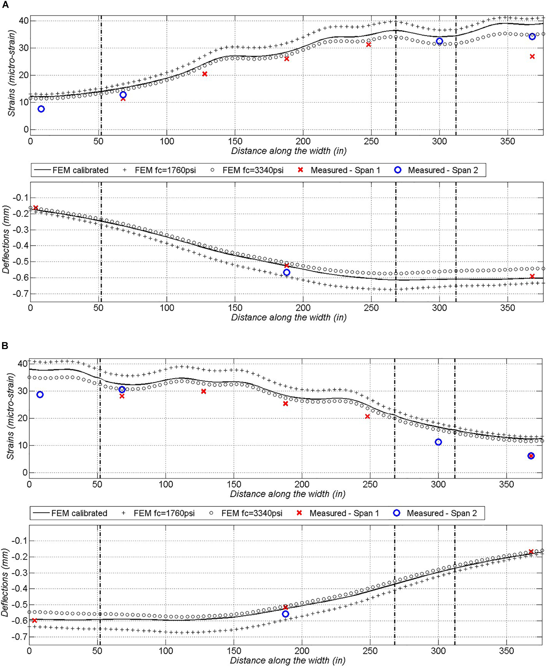
Figure 9. Comparison plot of strains and deflections for (A) LP-4-R, (B) LP-4-L (1 inch = 25.4 mm, 1 mm = 0.02 inch).

Due to the shape of the piers and span-to-thickness ratio, it was expected to see compressive stresses in the slab distribute in a shape of an arch. Figure 10, confirms this argument and shows a map of compressive stresses with tensile stress regions grayed-out.

FIGURE 10

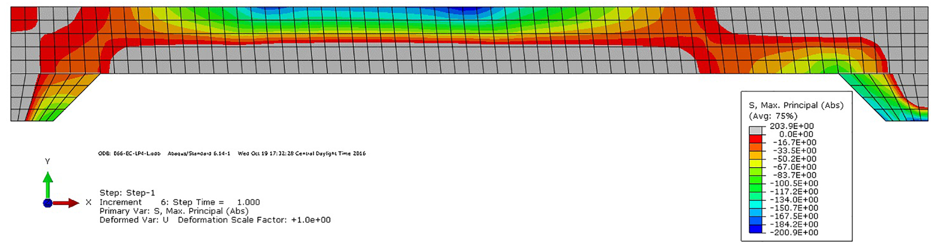
Figure 10. Cross-sectional view of principal stresses due to LP-4-L load configuration (1 inch = 25.4 mm, 1 mm = 0.02 inch).

Conclusion

This project illustrates how field measurements from GPR, UPV testing device, ACCM, core tests and live load tests were performed and used to define the structural details of a flat slab bridge. These details allowed to develop state-of-art non-linear FE model to determine the load capacity of the structure. Based on the field measurements it was found that cupped reinforcing bars were used in the oldest, original segment 3, back in 1915. For this segment it was established that one-third of the reinforcement was terminated at 3.5 ft (1.06 m) from each support. Values of deflections and strains recorded during the load tests were very small, as expected. Even for the most critical load pattern with two test trucks together in one span, the bridge did not crack. This confirms the overall good condition of the structure and its reserve flexural capacity. Measured values of strains and deflections show reasonable symmetry in bridge’s behavior, especially for the oldest part of the slab. The FE Model developed showed overall good correlation with the measured values of strain and deflection. FE Model confirmed that the strength of the structure, resulting in small values of strains and deflection under live load, comes from arching action which is strictly associated with the geometry of the bridge. Non-linear material model definitions allow the model to be used in numerical simulations of load carrying capacity.

Data Availability Statement

All datasets generated for this study are included in the article/supplementary material.

Author Contributions

PW: main author of the manuscript, conducted analytical modeling, and field studies. MK: performed live load measurements and preliminary analysis of the results. JS: co-PI on the research project and the lead professor. AN: was a PI of the research project.

Funding

The authors would like to acknowledge the financial support provided by Alabama Department of Transportation, ALDOT Research Project 930-889, and the efforts of many at ALDOT who provided guidance and assistance that were essential to ensure that this project concluded in a useful and practical result.

Conflict of Interest

At the time of study, PW and MK were affiliated at Auburn University. PW has since moved to COWI North America, Inc, and MK has since moved to PRIME AE. This has no impact on the study conducted.

The remaining authors declare that the research was conducted in the absence of any commercial or financial relationships that could be construed as a potential conflict of interest.

Acknowledgments

The research reported in this paper was conducted by authors being part of Highway Research Center at Auburn University, with the sponsorship of the Alabama Department of Transportation. Special thanks are due to Golpar Garmestani, Anjan Ramesh Babu, and Victor Aguilar who were graduate students also involved in this research project.

References

AASHTO, (2001). AASHTO Standard Specifications for Highway Bridges. Washington, DC: AASHTO.

Google Scholar

AASHTO, (2011). AASHTO Manual for Bridge Evaluation. Washington, DC: AASHTO.

Google Scholar

ABAQUS, (2014). Abaqus Analysis User’s Manual, Version 6.14. Vélizy-Villacoublay: Dassault Systèmes.

Google Scholar

Amer, A., Arockiassmy, M., and Shahawy, M. (1999). Load distribution of existing solid slab bridges based on field tests. J. Bridge Eng. 4, 189–193. doi: 10.1061/(asce)1084-0702(1999)4:3(189)

CrossRef Full Text | Google Scholar

American Concrete Institute, (2014). ACI 318-14 Building Code Requirements for Structural Concrete and Commentary. Farmington Hills, MI: American Concrete Institute.

Google Scholar

BDI, (2016a). LVDT – Displacement Sensor: Specification. Available online at: https://bditest.com/wp-content/uploads/LVDT (accessed August 13, 2019).

Google Scholar

BDI, (2016b). ST350 – Strain Transducer: Operations Manual. Available online at: https://bditest.com/wp-content/uploads/ST350-Strain-Transducer-Operations-Manual-v3.0.pdf (accessed August 13, 2019).

Google Scholar

Chajes, M. J., and Shenton, H. W. (2006). Using diagnostic load tests for accurate load rating of typical bridges. J. Bridge Struct. 2, 13–23. doi: 10.1080/15732480600730805

CrossRef Full Text | Google Scholar

Chaudhari, S. V., and Chakrabarti, M. A. (2012). Modeling of concrete for nonlinear analysis using finite element code abaqus. Int. J. Comput. Appl. 44, 14–18. doi: 10.5120/6274-8437

CrossRef Full Text | Google Scholar

Davids, W., and Tomlinson, S. (2016). Instrumentation During Live Load Testing and Load Rating of Five Reinforced Concrete Slab Bridges. Report 16-23-1332.3. Orono, ME: University of Maine.

Google Scholar

Davis, W. G., Poulin, T. J., and Goslin, K. (2013). Finite-Element Analysis and load rating of flat slab concrete bridges. J. Bridge Eng. 18, 946–956. doi: 10.1061/(asce)be.1943-5592.0000461

CrossRef Full Text | Google Scholar

Desayi, P., and Kirshnan, S. (1964). Equations for the stress-strain curve of concrete. J. Amer. Concr. Inst. 61, 345–350. doi: 10.3390/ma9050377

PubMed Abstract | CrossRef Full Text | Google Scholar

European Committee for Standarization, (2004). EN 1992-1-1: Design of Concrete Structures – Part 1-1: General Rules and Rules for Buildings. Brussels: European Committee for Standardization.

Google Scholar

Jáuregui, D., Licon-Lozano, A., and Kulkarni, K. (2010). Higher level evaluation of a reinforced concrete slab bridge. J. Bridge Eng. 15, 93–96.

Google Scholar

Kamiński, M., and Kmiecik, P. (2011). Modelling of reinforced concrete structures and composite structures with concrete strength degradation taken into consideration. Arch. Civil Mech. Eng. 11, 623–636. doi: 10.1016/s1644-9665(12)60105-8

CrossRef Full Text | Google Scholar

Logan, D. L. (2017). A First Course in the Finite Element Method, 6th Edn. Boston, MA: Cengage Learning.

Google Scholar

Sanayei, M., Phelps, J., Sipple, J., Bell, E. S., and Brenner, B. R. (2012). Instrumentation, nondestructive testing and finite-element model updating for bridge evaluation using strain measurements. J. Bridge Eng. 17, 130–138. doi: 10.1061/(asce)be.1943-5592.0000228

CrossRef Full Text | Google Scholar

Saraf, V. (1998). Evaluation of existing RC slab bridges. J. Perform. Const. Facil. 12, 20–24. doi: 10.1061/(asce)0887-3828(1998)12:1(20)

CrossRef Full Text | Google Scholar

Wang, T., and Hsu, T. T. C. (2001). Nonlinear finite element analysis of concrete structures using new constitutive models. Comput. Struct. 79, 2781–2791. doi: 10.1016/s0045-7949(01)00157-2

CrossRef Full Text | Google Scholar