Reinforcement Learning and Graph Embedding for Binary Truss Topology Optimization Under Stress and Displacement Constraints

1. Introduction

A number of methods based on a ground structure (GS) method (Dorn, 1964) have been proposed for topology optimization of trusses. GS method obtains a sparse optimal topology of trusses from a densely connected initial GS, where cross-sectional areas are chosen as continuous design variables. The complexity of GS ranges from Level-1, where all neighboring nodes are connected, to full level, where each node is connected to all the other nodes. Although full level GS is required in order to obtain a global optimal solution for the given nodes and the loading and boundary conditions, the combination of node pairs explodes to n_n(n_n − 1)/2 as the number of nodes n_n increases. For this reason, a truss with a limited number of members connecting to only adjacent nodes is frequently used as an initial GS, and GS grids with Level-1 connectivity are used in this paper. A generalized GS method with variable nodal locations can be used for also optimizing the geometry of a truss. The authors proposed a force density method for simultaneous optimization of topology and geometry of a truss (Ohsaki and Hayashi, 2017; Hayashi and Ohsaki, 2019).

However, it becomes difficult to obtain the global optimum even for the sparser initial GS stated above when stress constraints of the members are added to the optimization problem under multiple loading conditions, because the stress constraint can be neglected for a member whose cross-sectional area is reduced to zero during the optimization process (Kirsch, 1989; Ohsaki, 1995; Cheng and Guo, 1997; Achtziger and Stolpe, 2009). To overcome this discontinuity, branch-and-bound type techniques are proposed. Sheu and Schmit (1972) formulated a two-level optimization problem where existence of members and nodes varies in the upper-level linear optimization problem and they are fixed in the lower-level non-linear programming (NLP) problem. Ringertz (1986) improved the above method so as to consider displacement constraints in the lower-level problem; however, only small-scale trusses with 10–29 members are studied. Ohsaki and Katoh (2005) also adopted branch-and-bound approach to optimize trusses with constraints on stresses, nodal instability, and intersection of members; however, the number of LP steps and computational cost increase drastically as the size of problem is increased. Besides branch-and-bound type techniques for trusses with integer design variables, metaheuristic techniques such as genetic algorithms (Hajela and Lee, 1995) and simulated annealing (Topping et al., 1996) have been presented. A method heuristically adding nodes and members from a relatively sparse GS is also proposed (Hagishita and Ohsaki, 2009).

In the past decades, machine learning has been extensively studied in the field of structural engineering. Because the technique is developed to approximate a highly nonlinear function, the trained model is capable of predicting structural properties and behavior obtained through complex structural analysis, such as shear capacity of reinforced concrete beams (Prayogo et al., 2019), concrete compressive strength (Chou and Pham, 2013), and ground vibration induced by blasting (Khandelwal, 2011). The trained model is also used to accelerate iterative computation processes. Tamura et al. (2018) used a support vector machine and a decision tree to classify desirable and non-desirable brace placements of steel frames for application to optimization, and Papadrakakis et al. (1998) used a multilayer perceptron to predict the objective function value during size and shape optimization. Note that the researches stated above all belong to supervised learning that is a class of machine learning in which labeled input-output pairs must be provided.

Reinforcement learning (RL) is also an area of machine learning that aims to train an action taker called agent to take actions so as to maximize the cumulative rewards (Sutton and Barto, 1998). It differs from supervised learning because input-output pairs are not necessarily provided as learning material; instead, it requires a reward function that evaluates the output state. The trained agent overwhelmed human experts in playing Go (Silver et al., 2017) and some classic arcade games (Mnih et al., 2015); however, few applications have been studied in the field of structural engineering. Nakamura and Suzuki (2018) proposed an RL-based approach for selection between initial and tangential stiffness methods in the non-linear structural analysis; however, it dealt with a small solution space in which available actions are only two. Among a variety of machine learning methods, deep learning has recently attracted engineers because it showed remarkable results for complex tasks such as image recognition (Krizhevsky et al., 2012; He et al., 2015) and image generation (Goodfellow et al., 2014). Compared with conventional optimization methods that require high computational cost for iterative structural analyses, once the training process is finished, deep learning method is capable of yielding feasible solutions without any time-consuming iterative analysis process. Deep learning method showed considerable performance to predict sub-optimal material distribution for finite element models (Yu et al., 2018) and to select edge set that minimizes the total structural volume of a compression-only thrust network (Liew et al., 2019), which require high computational cost if conventional iterative schemes are used. However, the achievement above is strongly dependent on convolutional neural network (Lecun et al., 1998) that employs a mathematical operation called convolution specially designed for extracting the feature values from raster images formed by pixels in a rectangular array. For application of convolution to discrete structures, it is necessary to convert the structural model into a raster image in the same way as Yu et al. (2018) and Liew et al. (2019). For this reason, the method of convolution used for image processing cannot handle connectivity of discrete structures. Although Lee et al. (2018) utilized a multi-layer perceptron, a class of neural networks that does not employ convolutional layers, for predicting nodal displacements and member stresses of 10-bar trusses, the trained model cannot be applied to different trusses without modifying the structure of neural network and thus is not versatile.

Apart from convolutional neural networks, a number of graph embedding methods have been proposed to perform convolution on graphs instead of images (Cai et al., 2017), and they have shown a significant performance for multi-label network classification for social networking service (Perozzi et al., 2014) and prediction of chemical properties of organic molecules (Faber et al., 2017; Gilmer et al., 2017). Combination of RL and graph embedding may have a great potential. Dai et al. (2017) extracted node features using graph embedding, and the features are used to implement Q-learning (Watkins and Dayan, 1992) for typical NP-hard problems such as minimum vertex cover, maximum cut, and traveling salesman problems. Training was conducted for graphs with 50–100 nodes and the trained model shows good performance comparable to a benchmark mathematical programming solver for larger graphs with 1,000–1,200 nodes. However, this method identifies the nodes to be chosen, and it cannot be directly applied to truss topology optimization problem in which the edges for applying an operation are to be identified.

In this paper, we propose a combined method of graph embedding and RL for binary topology optimization of planar trusses for volume minimization under stress and displacement constraints. Note that the proposed method belongs to a binary type approach where the cross-sectional area of each member either keeps its initial value, or obtains a very small value. A variety of load and support conditions are provided for an initial GS, and removal of unnecessary members and updating of trainable parameters are implemented simultaneously and sequentially. The trained agent is not only capable of obtaining sub-optimal solutions at low computational cost, but also reusable to other trusses with different geometry, topology, and boundary conditions.

The remainder of this paper is organized as follows. The topology optimization problem focused in this study is first formulated in section 2. Next, the optimization problem is converted into an RL task, and then extracting member features and a Q-learning-based method using them are explained in section 3. Performance of the proposed method is demonstrated through numerical examples in section 4.

2. Topology Optimization of Trusses

2.1. Stiffness Method to Obtain Stress and Displacement

Displacements of nodes and axial stresses of members are computed for n_L static loading conditions using a standard stiffness method. Consider a planar truss with a total number of degree of freedom n_d, the number of members n_m, and the constant elastic modulus E. Let A_i and L_i denote the cross-sectional area and the length of member i. If only axial stiffness is considered for member stiffness, the member stiffness matrix with respect to the local coordinates of member i is a matrix ${\text{K}}_i\in {ℝ}^{4\times 4}$ where (1, 1) and (3, 3) elements are EA_i/L_i and (1, 3) and (3, 1) elements are −EA_i/L_i. Member stiffness matrices of all the members are transformed into the global coordinate system to be assembled to the global stiffness matrix $\text{K}\in {ℝ}^{n_{\text{d}}\times n_{\text{d}}}$. Using K, nodal displacements are obtained by solving the following stiffness equation:

$\begin{array}{ll}\text{K}{\text{u}}_j={\text{p}}_j& (1)\end{array}$

where ${\text{u}}_j\in {ℝ}^{n_{\text{d}}}$ and ${\text{p}}_j\in {ℝ}^{n_{\text{d}}}$ are the nodal displacement and the nodal load vectors corresponding to the load case j ∈ {1, ⋯ , n_L}. Let σ_{i, j} denote the axial stress of member i for the load case j, which is expressed as

$\begin{array}{ll}{\sigma }_{i,j}=\frac{E{d}_{i,j}}{L_i}& (2)\end{array}$

where d_{i, j} is the elongation of member i for load case j, which is simply calculated after obtaining the nodal displacements.

2.2. Optimization Problem

Let A = {A₁, ⋯ , A_nm} denote the vector of cross-sectional areas. This research aims to obtain the optimal topology of a truss that minimizes the total structural volume V(A) under stress constraints. However, some solutions to this problem are trivial; for example, if all the members connecting to supporting nodes are eliminated, the structure cannot resist against external loads at all while the stress constraints for existing members are satisfied. For this reason, displacement constraints are further added to avoid apparently infeasible trusses that deform excessively. By assigning the upper-bound stress $\bar{\sigma }$ and the upper-bound displacement ū, the optimization problem is formulated as follows:

$\begin{array}{ll}\text{minimize }V(\text{A})& (\mathrm{3a})\end{array}$

$\begin{array}{ll}\text{subject to }{\displaystyle \underset{i\in {\Omega }_{\text{m}},j\in \left\{1,\cdots ,n_{\text{L}}\right\}}{\text{max}}}\left(\frac{|{\sigma }_{i,j}(\text{A})|}{\bar{\sigma }}\right)\le 1& (\mathrm{3b})\end{array}$

$\begin{array}{ll}{\displaystyle \underset{i\in {\Omega }_{\text{d}},j\in \left\{1,\cdots ,n_{\text{L}}\right\}}{\text{max}}}\left(\frac{|u_{i,j}(\text{A})|}{ū}\right)\le 1& (\mathrm{3c})\end{array}$

$\begin{array}{ll}{A}_i\in \left\{Ā\times 10^{-6},Ā\right\}(i=1,\cdots ,n_{\text{m}})& (\mathrm{3d})\end{array}$

where Ω_m and Ω_d are the sets of indices of existing members and DOFs of existing nodes including loaded nodes, and u_{i, j} is the ith displacement component for load case j. Hereafter, the ratio $\left|{\sigma }_{i,j}\right|/\bar{\sigma }$ is called stress safety ratio, which indicates a safe state if it is small. The cross-sectional areas are chosen from Ā for existing members and a small value Ā × 10⁻⁶ instead of 0 for non-existing members to prevent singularity of the stiffness matrix K in Equation (1).

3. Training for Removal of Members

3.1. Re-formulation as Reinforcement Learning Task

The RL task needs to be formulated as a Marcov decision process (Bellman, 1957): a discrete time stochastic process where state transition and reward function are solely dependent on the current state and the chosen action, and are independent of the previous states and actions. A Marcov decision process comprises four elements S, A, P, R, where S and A are the state and action spaces, and P and R are the transition probability function and the reward function to observe the next state s′ and reward r by taking an action a at the current state s, respectively. Some states are set as terminal states, and tasks reaching them are terminated.

In the following, we re-formulate the truss topology optimization problem utilizing RL tasks. For this purpose, it is desirable for a state to include numerical data of a truss as many as possible. Here, a state is represented as a set of numerical data at nodes v = {v₁, …, v_nn} and that of members w = {w₁, …, w_nm}, as described in Tables 1, 2 based on the loading and support conditions, geometry of the truss, and the stress safety ratios. In Table 1, the load intensity is defined as the magnitude of the external load applied at the node, which is decomposed into x and y directions; the magnitude in z direction is omitted because only planar trusses are focused in this study. In Table 1, the orientation of member is expressed by trigonometric quantities cosα and sinα instead of angle α so as to avoid discontinuity at α = 0 = 2π. Note that connectivity of nodes is not considered here as it can be expressed by graph embedding described later.

TABLE 1

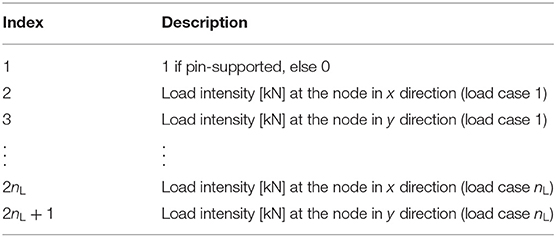
Table 1. Description of node state data v_k for nodes.

TABLE 2

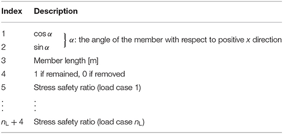
Table 2. Description of member state data w_i for members.

Action is defined as elimination of a member from existing ones. Note again that the members regarded as removed virtually have a very small cross-sectional area as seen in Equation (3D) to avoid instability in computing nodal displacements. The description of transition probability function P is omitted because any state-action pair deterministically leads to a unique next state. Reward is evaluated after each removal of a member. When the truss violates stress or displacement constraints, reward of −1 is provided and removal process is terminated. Otherwise, the reward computed by the following equation is provided:

$\begin{array}{ll}r=L_{\text{e}}\left(1-{\displaystyle \underset{i\in {\Omega }_{\text{m}},j\in \left\{1,\cdots ,n_{\text{L}}\right\}}{\text{max}}}\frac{|{\sigma }_{i,j}|}{\bar{\sigma }}\right)& (4)\end{array}$

where L_e is the length of the eliminated member. Equation (4) is derived considering the total structural volume to be minimized and the stress safety ratio to be constrained; accordingly, the reward is large when the eliminated member is long and the maximum stress safety ratio of the resulting topology is small.

The action taker is called agent in the field of RL. Agent simultaneously updates its policy π while taking an action and observing the next state and reward at each step. This way, the agent learns from experience, which is a unique property of RL. The policy is determined based on the expected cumulative reward; in particular, summation of the expected reward taking an action a at state s and following the policy π hereafter is called action value Q^π(s, a). One of the simplest policies is a greedy policy that determines an action expected to obtain the maximum expected cumulative reward, computed as:

$\begin{array}{ll}\pi (s)={\displaystyle \underset{a\in {\Omega }_{\text{m}}}{\text{argmax }}}Q(s,a)& (5)\end{array}$

where a = i selecting the indice i from the set Ω_m means the action to remove member i. However, deterministic policies such as the greedy policy are inefficient in exploring better solutions, and an ϵ-greedy policy, as follows, is preferred as a policy utilized during training:

$\begin{array}{ll}\pi (s)=\{\begin{array}{cc}{\displaystyle \underset{a\in {\Omega }_{\text{m}}}{\text{argmax }}}Q(s,a)\hfill & (\text{if random }\left[0,1\right]>ϵ)\hfill \\ \text{random }a\text{ from }{\Omega }_{\text{m}}\hfill & (\text{else})\hfill \end{array}\hfill & (6)\end{array}$

The difference of the ϵ-greedy policy from the standard greedy policy is that it chooses an action randomly with low probability ϵ and this randomness improves exploration. However, a problem arises due to curse of dimensionality (Bellman, 1961); it is impossible to compute and preserve action values for all the possible state-action pairs when the state and action spaces are too large. In this paper, there are a variety of properties for state representation of the truss, and the state space is too large even for small-scale trusses. For such a case, a function approximation is often used because the action values can be expressed by a relatively small number of parameters. In the next section, truss structures are regarded as graphs and the action values to eliminate a member are estimated by graph embedding.

3.2. Action Value Estimated by Graph Embedding

Truss structures can be modeled as graphs. In this section, features of each member are represented as a vector by aggregating numerical data about neighbor nodes and members. Let n_f denote the size of the feature vector of a member, which is to be determined through careful adjustment with trial-and-error for better performance, because too small size leads to inaccuracy in expressing the features, and too large size requires redundant computation time in training and application of the agent after training. Using the parameters ${\theta }_1\in {ℝ}^{n_{\text{f}}\times (n_{\text{L}}+4)}$, ${\theta }_2\in {ℝ}^{n_{\text{f}}\times n_{\text{f}}}$, ${\theta }_3\in {ℝ}^{n_{\text{f}}\times (2n_{\text{L}}+1)}$, ${\theta }_4\in {ℝ}^{n_{\text{f}}\times n_{\text{f}}}$, ${\theta }_5\in {ℝ}^{n_{\text{f}}\times n_{\text{f}}}$, and ${\theta }_6\in {ℝ}^{n_{\text{f}}\times n_{\text{f}}}$ that are to be trained, the feature vector of each member ${\mu }_i\in {ℝ}^{n_{\text{f}}}(i=1,\cdots ,n_{\text{m}})$ is updated as follows:

$\begin{array}{ll}{\mu }_i^{(0)}=\text{0}& (\mathrm{7a})\end{array}$

$\begin{array}{ll}{\mu }_i^{(t+1)}=\text{ReLU}\left({\text{h}}_1+{\text{h}}_2+{\text{h}}_3^{(t)}+{\text{h}}_4^{(t)}\right)& (\mathrm{7b})\end{array}$

$\begin{array}{ll}{\text{h}}_1={\theta }_1{\text{w}}_i& (\mathrm{7c})\end{array}$

$\begin{array}{ll}{\text{h}}_2={\theta }_2{\displaystyle \sum _{j=1}^2}\text{ReLU}\left({\theta }_3{\text{v}}_{i,j}\right)& (\mathrm{7d})\end{array}$

$\begin{array}{ll}{\text{h}}_3^{(t)}={\theta }_4{\mu }_i^{(t)}& (7e)\end{array}$

$\begin{array}{ll}{\text{h}}_4^{(t)}={\theta }_5{\displaystyle \sum _{j=1}^2}\text{ReLU}\left({\theta }_6{\displaystyle \sum _{k\in {\Phi }_{i,j}}}{\mu }_k^{(t)}\right)& (\mathrm{7f})\end{array}$

where t is the step number of updating the features, v_{i, j} is the nodal features of jth (j ∈ {1, 2}) end of member i, and Φ_{i, j} is the set of indices of members connecting to jth end of member i. Note that Φ_{i, j} does not include the index of member i itself. ReLU is a rectifier linear unit function: one of activation functions, which is defined as:

$\begin{array}{ll}\text{ReLU}(b)=\{\begin{array}{cc}b\hfill & (\text{if }b>0)\hfill \\ 0\hfill & (\text{else})\hfill \end{array}\hfill & (8)\end{array}$

An activation function needs to be nonlinear in order to approximate a nonlinear function and differentiable in order to apply a gradient based optimization algorithm. ReLU is widely used as an activation function for neural networks although it is not differentiable at 0, because the computational cost to compute its gradient is very small and the gradient does not vanish even when input is a large positive value. To simplify the expression, the ReLU function is applied in Equation (7) to a vector to output a vector of the same size.

The operation in Equation (7) is illustrated in Figure 1. The numerical data of two nodes and members connecting to them is aggregated into the feature vector of a member through a single operation. The aggregated numerical data include member state data in Equation (7C), connecting nodes' state data in Equation (7D), embedded feature of the member itself in Equation (7E), and embedded features of neighboring members in Equation (7F). Accordingly, $\left\{{\mu }_1^{(t)},\cdots ,{\mu }_{n_{\text{m}}}^{(t)}\right\}$ is the set of feature vectors incorporating connectivity of the truss after ${\mu }_i^{(t)}$ for all the members is computed from Equation (7); however, this should be iterated more than once because the values of ${\mu }_i^{(t)}$ for neighbor members interact with each other. In accordance with the previous research of Dai et al. (2017), the number of iteration T is set to be 4. It should be noted that the embedded feature vector ${\mu }_i^{(T)}$ has the same size n_f regardless of connectivity. Owing to this property, all the members can be evaluated based on the same measure hereafter.

FIGURE 1

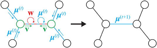
Figure 1. The concept of Equation (7). It aggregates numerical data of neighbor nodes and members.

Using $\widehat{\mu }=\left\{{\mu }_1^{(T)},\cdots ,{\mu }_{n_{\text{m}}}^{(T)}\right\}$, the action value to eliminate member i in the current state is approximated using trainable parameters ${\theta }_7\in {ℝ}^{2n_{\text{f}}}$, ${\theta }_8\in {ℝ}^{n_{\text{f}}\times n_{\text{f}}}$, and ${\theta }_9\in {ℝ}^{n_{\text{f}}\times n_{\text{f}}}$ as follows:

$\begin{array}{ll}Q(\widehat{\mu },i)={\theta }_7^{\top }\left(\text{ReLU}\left[{\theta }_8{\displaystyle \sum _{i=1}^{n_{\text{m}}}}{\mu }_i^{(T)};{\theta }_9{\mu }_i^{(T)}\right]\right)& (9)\end{array}$

where [·;·] is a concatenation operator of two vectors in the column direction. Since $\widehat{\mu }$ is also computed using {θ₁, ⋯ , θ₆}, the action value $Q(\widehat{\mu },i)$ is dependent on Θ = {θ₁, ⋯ , θ₉}. The training method for tuning the parameters Θ is described below.

3.3. Q-Learning Using the Embedded Features

The parameters Θ are tuned using a method based on 1-step Q-learning method, which is a frequently used RL method. When a function approximator is not utilized, the action value is updated using state s, chosen action a, observed next state s′ and reward r as:

$\begin{array}{ll}Q(s,a)=Q(s,a)+\alpha \left(r(s^{\prime })+\gamma {\displaystyle \underset{a}{\text{max}}}Q(s^{\prime },a)-Q(s,a)\right)& (10)\end{array}$

where α > 0 is a learning rate that has an effect on convergence of the training. γ ∈ [0, 1] is a discount factor; i.e., the action value becomes closer to expected cumulative reward as γ is larger, and conversely, the action value becomes closer to expected instant reward as γ is smaller. In other words, γ should be closer to 1 if future and instant rewards are equivalently important, and 0 if only instant reward is important. In Equation (10), the action value is updated so as to minimize the difference between the sum of observed reward and estimated action value at the next state $r(s^{\prime })+\gamma \underset{a}{max}Q(s^{\prime },a)$ and estimated action value at the previous state Q(s, a). Following this scheme, the parameters are trained by solving the following optimization problem (Mnih et al., 2015):

$\begin{array}{ll}minimizeF(\text{Θ})={\left(r(s^{\prime })+\gamma {\displaystyle \underset{ã}{\text{ max }}}Q(s^{\prime },ã;\widetilde{\text{Θ}})-Q(s,a;\text{Θ})\right)}^2& (11)\end{array}$

In Equation (11), the training can be stabilized by using parameters $\widetilde{\text{Θ}}$ at the previous state for estimation of the action value at the next state s′ (Mnih et al., 2015). In the same manner as neural networks, a back-propagation method (Rumelhart et al., 1986), which is a gradient based method to minimize the loss function, can be used for solving Equation (11). RMSprop (Tieleman and Hinton, 2012) is adopted as the optimization method in this study.

3.4. Training Workflow

The whole training workflow is described in Figure 2. The inputs are the initial GS, the bounds for stress and displacement, and the graph embedding class that contains trainable parameters Θ initialized by the vectors with the sizes defined by n_L and n_f. Although stress and displacement bounds have the same value $\bar{\sigma }$ and ū, respectively, for each member and DOF in this study, it should be noted that each member could have a different stress bound and each DOF could have a different displacement bound for each load case, which provides a versatility to the proposed method.

FIGURE 2

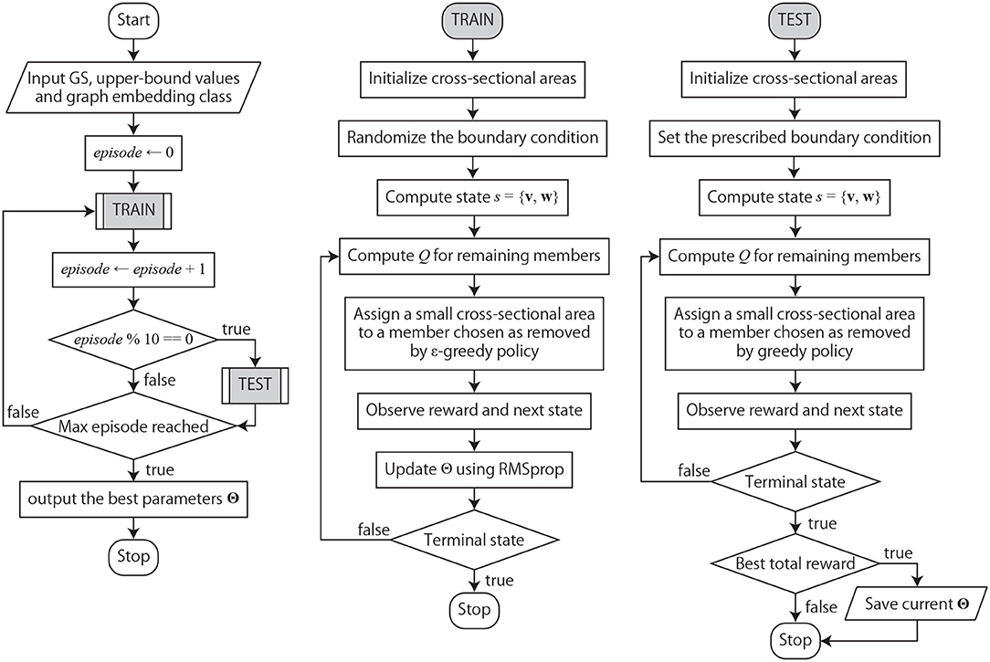
Figure 2. Training workflow utilizing RL and graph embedding.

An episode is defined as a sequence of member removal process from the initial GS to the terminal state violating constraints. Load and support conditions are randomly provided according to a rule so that the agent can be trained to have good performance for various boundary conditions. To reduce the required capacity of a storage device, 1,000 sets of observed transitions (s, a, s′, r) are stored at the maximum. When the number of transition steps reaches 1,000, the latest transition overrides the oldest one. In the optimization with RMSprop, 32 datasets out of the stored transitions are randomly chosen to create a minibatch and the set of trainable parameters Θ is updated based on the mean squared error of the loss function of each dataset computed by the right-hand side of Equation (11). In this study, γ = 0.99 is adopted, because cumulative reward indicating the amount of reduction of structural volume as a result of the action is much more important than the instant reward. The number of training episodes is set as 5,000.

Once in 10-episode training, the performance of Θ is tested for prescribed loading and boundary conditions. The cumulative reward until terminal state is recorded using the greedy policy without randomness (i.e., ϵ-greedy policy with ϵ = 0) during the test. If the cumulative reward is larger than the previous best score, Θ at that step is saved. Θ saved after the 5,000-episode training is regarded as the best parameters.

4. Numerical Examples

The agent is trained and its performance is tested for a simple planar truss in section 4.1. The performance is also tested for other different trusses in sections 4.2–4.4 without re-training the results in section 4.1. We use a PC with a CPU of Intel(R) Core(TM) i9-7900X @ 3.30GHz. The program is implemented within Python 3.7 environment.

The upper-bound stress $\bar{\sigma }$ is 200 N/mm² for both tension and compression for all examples. The upper-bound displacement ū for each boundary condition is computed by multiplying 100 to the maximum absolute value of displacement among the all DOFs of the initial GS with the same loading and boundary conditions; hence, ū varies depending on the structure and the loading and boundary conditions. The initial cross-sectional area is 1,000 mm², and the elastic modulus is 2.0 × 10⁵ N/mm² for all members of all examples. The number of loading conditions is fixed as n_load= 2, and accordingly, the sizes of inputs from nodes and members are 5 and 6, respectively. The size of embedded member feature n_f is 100.

4.1. 4 × 4-Grid Truss

The agent is trained using a 72-member truss with 4 × 4 grids. The initial GS is illustrated in Figure 3. Each grid is a square whose side length is 1 m. The intersection of bracing members is not connected. The boundary conditions are given at the beginning of each episode. Two pin-supports are randomly chosen; one from nodes 1 and 2 and the other from nodes 4 and 5. Right tip nodes are candidates to apply loading, and a horizontal or a vertical load with the fixed magnitude of 1.0 kN is applied at a randomly chosen node. Note that it is possible that the two load cases are identical, or applied to different nodes but in the same direction. Consequently, the training concerns a total of 2 × 2 × 20 × 20 = 1, 600 combinations of support and loading conditions, and these combinations are almost equally simulated as long as the number of training episodes are sufficient.

FIGURE 3

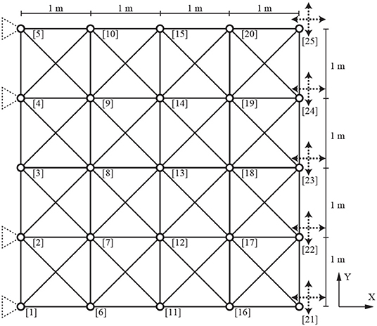
Figure 3. Example 1: 4 × 4-grid truss (V = 0.0853 [m³]).

During the test, nodes 1 and 5 are pin-supported, and loads are applied at node 23 in positive x and negative y direction separately as different loading conditions, which is denoted as loading condition L1. Figure 4 plots the history of cumulative rewards in the test simulation recorded at every 10 episodes. The score rapidly improves in the first 1,000 episodes and the score mostly keeps above 35.0 after 2,000 episodes. It is confirmed from this history that the agent successfully improves its policy to eliminate unnecessary members as the training proceeds. It took about 3.9 h for training through about 235,000 linear structural analyses. The maximum test score of 43.5 is obtained at the 2,100th episode, and the parameter Θ at this episode is dealt as the best parameters and used hereafter.

FIGURE 4

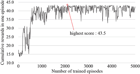
Figure 4. History of cumulative reward of each test measured every 10 episodes.

The removal sequence of members when the maximum score is recorded is illustrated in Figure 5. Note that the nodes highlighted in blue are pin-supported, those in yellow are loaded. Trivial members close to pin-supports or placed upper-right or bottom-right that do not bear stress are first removed, and important members along the load path are removed afterwards. This is an evidence that the agent is capable of detecting the load path among members, and we estimate that this capability is mainly due to graph embedding because it extracts member features considering truss connectivity.

FIGURE 5

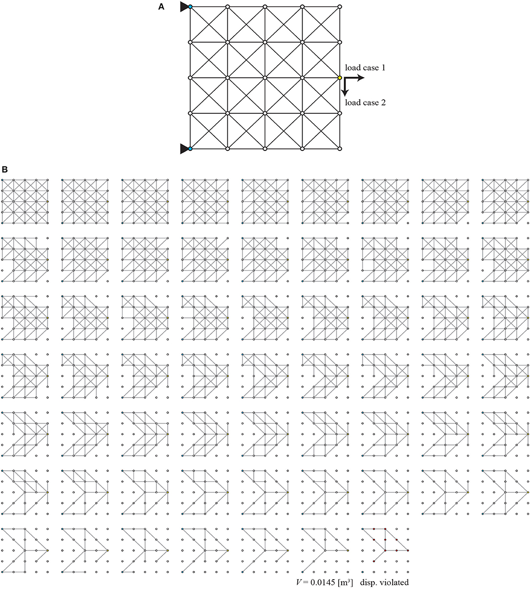
Figure 5. Best scored removal process of members for loading condition L1 of Example 1; (A) initial GS, (B) removal sequence to the terminal state.

The final truss of removal process of members presented in Figure 5 is a terminal state, where displacement constraint is violated at the nodes highlighted in red. Therefore, the topology just before the terminal state shall be a sub-optimal topology, which is a truss with 12 members as shown in Figure 5B. Since removal of any remaining member will cause violation of the displacement constraint, there is no unnecessary member in the sub-optimal topology. It forms a very simple truss composed of six pairs of members connecting linearly. Note that the connection between the members in each pair is an unstable node, and must be fixed to generate a single long member.

To investigate performance of the agent for another loading condition, the structure with the loads as shown in Figure 6A, denoted as loading condition L2, is also optimized using the same agent. Nodes 1 and 5 are pin-supported and nodes 22 and 24 are subjected to 1 kN load in positive x direction separately as two load cases. The removal sequence of members is illustrated in Figure 6B. Similarly to loading condition L1 in Figure 5, several symmetric topologies are observed during the removal process, and the sub-optimal topology is a well-converged solution that does not contain unnecessary members. From these results, the agent is confirmed to behave well for a different loading condition.

FIGURE 6

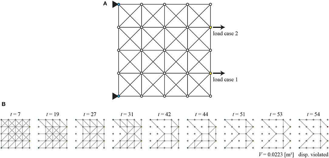
Figure 6. Loading condition L2 of Example 1; (A) initial GS, (B) removal sequence of members.

Furthermore, the robustness of the proposed method is also investigated by implementing 2,000-episode training using different random seeds for 20 times. The statistical data with respect to the maximum test score for each training are as follows; the average is 43.38, the standard deviation is 0.16, and the coefficient of variation is only 3.80 × 10⁻³. Moreover, all the trained RL agents with the best parameters led to the same 12-member sub-optimal solution as Figure 5B for loading condition L1. These results imply that the proposed method is robust against randomness of boundary conditions and actions during the training.

4.2. Investigation of Generalization Performance 1: 3 × 2-Grid Truss

The agent trained in Example 1 is reused for a smaller 3 × -grid truss without re-training. Figure 7 shows the initial GS. The edge length of each grid is 1 m also for this Example 2. Topology is optimized for two boundary conditions.

FIGURE 7

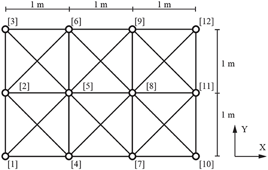
Figure 7. Example 2: 3 × 2-grid truss (V = 0.0340 [m³]).

In the first boundary condition B1, as shown in Figure 8A, left tip nodes 1 and 3 are pin-supported and bottom-right nodes 7 and 10 are subjected to downward unit load of 1 kN separately as different loading cases. As shown in Figure 8B, the agent utilizes an reasonable policy to eliminate obviously unnecessary members connecting to supports at first, non-load-bearing members around the supports next, and members in the load path at last. From this result, it is confirmed that the agent is capable of eliminating unnecessary members properly for a different-scale truss. The topology two steps before the terminal state contains successive V-shaped braces and is stable and statically determinate. The one just before the terminal state is a sub-optimal truss; however, instability exists at the loaded node.

FIGURE 8

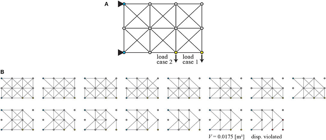
Figure 8. Boundary condition B1 of Example 2; (A) initial GS, (B) removal sequence of members.

In the second boundary condition B2, the bottom center nodes 4 and 7 are pin-supported and upper tip nodes 3 and 12 are subjected to outward unit loads along x axis as shown in Figure 9A. Similarly to the boundary condition B1, the agent eliminates members that do not bear forces as shown in Figure 9B. At the 18th step, a tower-like symmetric topology is created with extending members from upper tips to loaded nodes. After the 18th step, the topology became asymmetric despite the symmetry of problem definition; however, the asymmetric solutions should be accepted, because Guo et al. (2013) explained that solving the quasi-convex symmetric optimization problem may yield highly asymmetric solution.

FIGURE 9

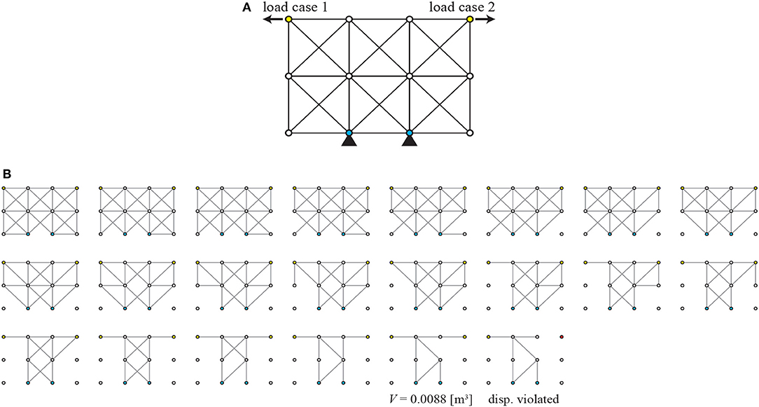
Figure 9. Boundary condition B2 of Example 2; (A) initial GS, (B) removal sequence of members.

4.3. Investigation of Generalization Performance 2: 6 × 6-Grid Truss

As Example 3, the agent is applied to a larger-scale truss, as shown in Figure 10, without re-training. The GS consists of 6 × 6 grids and the number of members is more than twice of the 4 × 4-grid truss. The truss is optimized for two loading conditions.

FIGURE 10

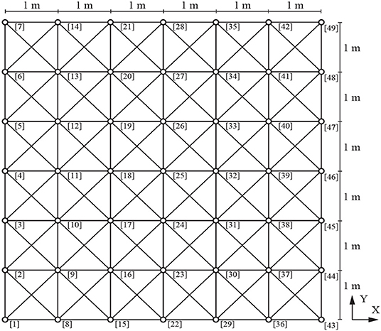
Figure 10. Example 3: 6 × 6-grid truss (V = 0.1858 [m³]).

The left two corners 1 and 7 are pin-supported and rightward and downward unit loads are separately applied at the bottom-right corner 43, as shown in Figure 11A in the loading condition L1. Topologies at steps 37, 60, 84, 100, 144, and 145 in the removal sequence are illustrated in Figure 11B. Although the agent is applied to a larger-scale truss, a sparse optimal solution is successfully obtained.

FIGURE 11

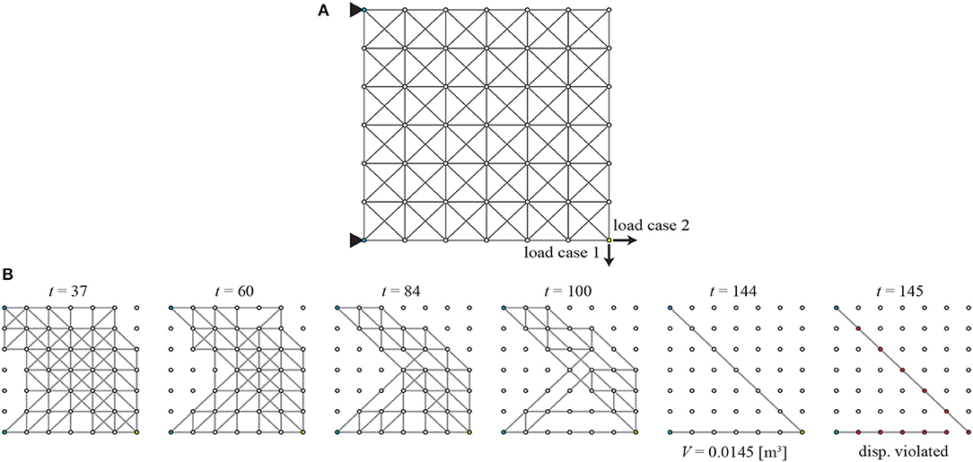
Figure 11. Loading condition L1 of Example 3; (A) initial GS, (B) removal sequence of members.

In the loading condition L2, the left two corners are again pin-supported, and the outward unit load is separately applied at nodes 4 and 46, as shown in Figure 12A. One of the loads applied at node 4 is an irregular case where pin-supports and the loaded node aligns on the same straight line. Even in this irregular case, the agent successfully obtained the sparse optimal solution, as shown in Figure 12. Moreover, during the removal process, there is almost no isolated member apart from load-bearing ones and existing members efficiently transmit forces to the supports.

FIGURE 12

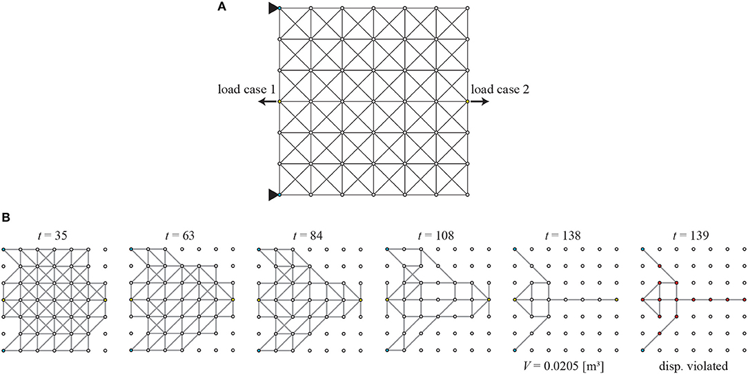
Figure 12. Loading condition L2 of Example 3; (A) initial GS, (B) removal sequence of members.

4.4. Comparison of Efficiency and Accuracy With Genetic Algorithm

The above examples using the proposed method are further investigated in view of efficiency and accuracy through comparison with genetic algorithm (GA). GA is one of the most prevalent metaheuristic approach for binary optimization problems, which is inspired by the process of natural selection (Mitchell, 1998). In GA, a set of solutions are repeatedly modified using the operations such as selection, where superior solutions at current generation are selected for new generation, crossover, where the selected solutions are combined to breed child solutions sharing the same characteristics as the parents, and mutation, where the selected solutions randomly change their values with low probability. A simple GA algorithm used in this section is explained in Algorithm 1. This algorithm is terminated if the best cost function value f_b is not updated for n_s = 10 consecutive generations.

ALGORITHM 1

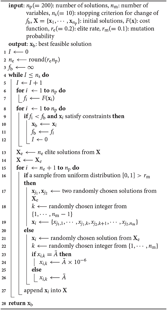
Algorithm 1. Genetic algorithm used in this study

Because the optimization problem (Equation 3) contains constraint functions, the cost function F used in GA is defined using the penalty term as:

$\begin{array}{ll}F(\text{A})=V(\text{A})+{\beta }_1{C}_1(\text{A})+{\beta }_2{C}_2(\text{A})& (\mathrm{12a})\end{array}$

$\begin{array}{ll}{C}_1(\text{A})=\text{max}\left\{\left({\displaystyle \underset{i\in {\Omega }_{\text{m}},j\in \left\{1,\cdots ,n_{\text{L}}\right\}}{\text{max}}}\left(\frac{|{\sigma }_{i,j}(\text{A})|}{\bar{\sigma }}\right)-1\right),0\right\}& (\mathrm{12b})\end{array}$

$\begin{array}{ll}{C}_2(\text{A})=\text{max}\left\{\left({\displaystyle \underset{i\in {\Omega }_{\text{d}},j\in \left\{1,\cdots ,n_{\text{L}}\right\}}{\text{max}}}\left(\frac{|u_{i,j}(\text{A})|}{ū}\right)-1\right),0\right\}& (\mathrm{12c})\end{array}$

where β₁ and β₂ are penalty coefficients for stress and displacement constraints; both are set to be 1000 in this study. If stress and displacement constraints are satisfied, penalty terms become zero and the cost function becomes equivalent to the total structural volume V(A). The same material property and constraints as the examples of RL are applied to the following problems. GA algorithm is run for 10 times with different initial solutions that are generated randomly, and only the best result that yields a solution with the least total structural volume is provided in the GA column in Table 3.

TABLE 3

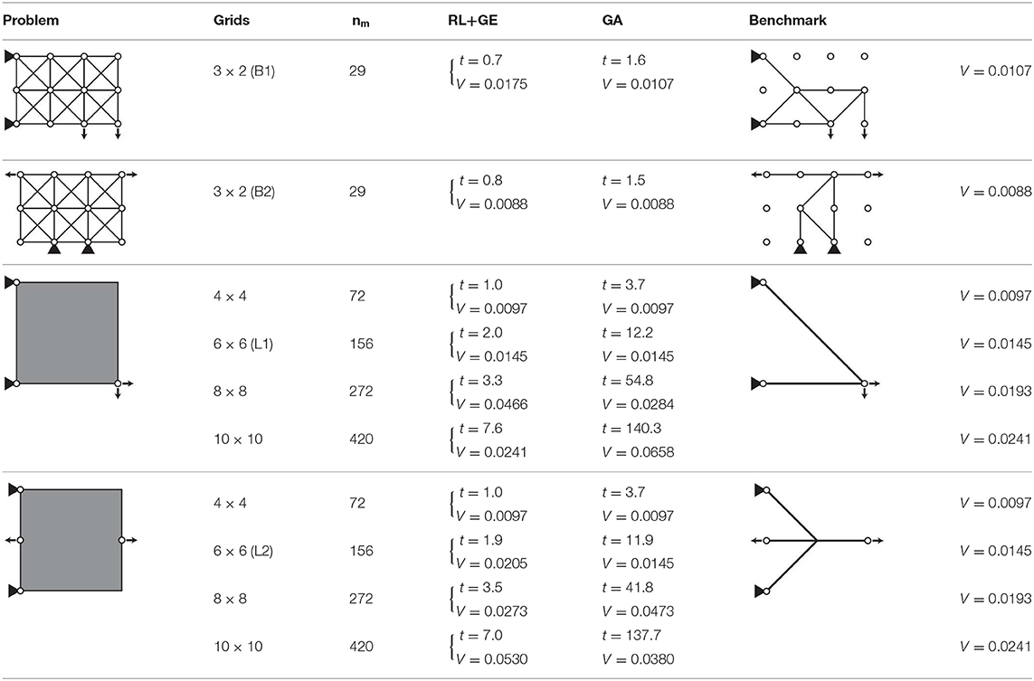
Table 3. Comparison between proposed method (RL+GE) and GA in view of total structural volume V[m³] and CPU time for one optimization t[s] using benchmark solutions.

The benchmark solutions for the 3 × 2-grid truss provided in Table 3 are global optimal solutions; this global optimality is verified through enumeration which took 44.1 h for each boundary condition. The other solutions are assumed to be global optima which have not been verified through enumeration due to extremely high computational cost.

In utilizing the trained agent in Example 1, n_load! different removal sequences can be obtained for different order of the same set of load cases in node state data v_k; for example, exchanging the values at indices 2 and 4 and those at indices 3 and 5 in v_k maintains the original loading condition but may lead to different action to be taken during each member removal process, because the neural network outputs different Q values due to the exchange. Although n_load! = 2 different removal sequences can be obtained in this way, only the better result with less total structural volume is provided in the RL+GE column in Table 3. Note that the total CPU time t[s] for obtaining this removal sequence of members includes initialization of the truss structure, import of the trained RL agent, and computing the removal sequence.

According to Table 3, the proposed RL+GE method is much more efficient than GA; the CPU time exponentially increases as the number of variable increases in GA; on the other hand, the CPU time increases almost linearly in RL+GE. The proposed method is also comparable to GA with n_p = 200 in terms of proximity to the global optimum; RL+GE generally reached the feasible solutions with less total structural volume compared with the solutions obtained by GA. In addition, the accuracy of the trained agent is less dependent on the size of the problem; the trained agent reached presumable global optimum for 10 × 10-grid truss with L1 loading condition, although the agent was caught at the local optimum for 8 × 8-grid truss with the same loading condition, and even for 3 × 2-grid truss with B1 boundary condition.

5. Conclusion

In this paper, a machine-learning based method combining graph embedding and Q-learning is proposed for binary truss topology optimization to minimize total structural volume under stress and displacement constraints. Although the use of CNN-based convolution method is difficult to apply to trusses as they cannot be handled as pixel-wise data, the convolution is successfully implemented for trusses by introducing graph embedding, which has been extended in this paper from the standard node-based formulation to a member(edge)-based formulation. This way, features of each member considering connectivity can be extracted. Using the features, the method to estimate the action value with respect to removal of the member is further formulated. The trainable parameters are optimized by a back-propagation method to minimize the loss function computed by estimated action value and observed reward.

It is verified from the numerical examples that the trained agent acquired a policy to reduce total structural volume while satisfying the stress and displacement constraints. Although it takes a long time for the training, the trained agent requires very low computational cost compared with GA at the application stage. Furthermore, the trained agent is applicable to a truss with different topology, geometry and loading and boundary conditions after it is trained for a specific truss with various loading and boundary conditions. This applicability was demonstrated through both smaller-scale and larger-scale trusses and sparse sub-optimal topologies were obtained for both cases. It is notable that the agent was able to optimize the structure with the unforeseen boundary conditions which the agent has never experienced during the training. It implies that the agent possesses generalized performance for a complex structural optimization task. However, in order to create a more reliable agent, it is necessary to implement the training with various topology, geometry, and loading and boundary conditions. Another approach may be to incorporate a rule-based method to create a hybrid optimization agent.

It is also advantageous that the agent is easily replicated and available in other computers by importing the trained parameters. The proposed method for training agent is expected to become a supporting tool to instantly feedback the sub-optimal topology and enhance our design exploration.

Data Availability Statement

The datasets generated for this study are available on request to the corresponding author.

Author Contributions

KH designed the study, implemented the program, and wrote the initial draft of the manuscript. MO contributed to problem formulation and interpretation of data, and assisted in the preparation of the manuscript. KH and MO approved the final version of the manuscript, and agree to be accountable for all aspects of the work in ensuring that questions related to the accuracy or integrity of any part of the work are appropriately investigated and resolved.

Funding

This work was kindly supported by Grant-in-Aid for JSPS Research Fellow No.JP18J21456 and JSPS KAKENHI No. JP18K18898.

Conflict of Interest

The authors declare that the research was conducted in the absence of any commercial or financial relationships that could be construed as a potential conflict of interest.

References

Achtziger, W., and Stolpe, M. (2009). Global optimization of truss topology with discrete bar areas-part ii: implementation and numerical results. Comput. Optim. Appl. 44, 315–341. doi: 10.1007/s10589-007-9152-7

CrossRef Full Text | Google Scholar

Bellman, R. (1957). A Markovian decision process. Indiana Univ. Math. J. 6, 679–684. doi: 10.1512/iumj.1957.6.56038

CrossRef Full Text | Google Scholar

Bellman, R. (1961). Adaptive Control Processes. (Princeton, NJ: Princeton University Press). doi: 10.1515/9781400874668

PubMed Abstract | CrossRef Full Text | Google Scholar

Cai, H., Zheng, V. W., and Chang, K. C. (2017). A comprehensive survey of graph embedding: problems, techniques and applications. IEEE Trans. Knowl. Data Eng. 30, 1616–1637. doi: 10.1109/TKDE.2018.2807452

CrossRef Full Text | Google Scholar

Cheng, G., and Guo, X. (1997). ε-relaxed approach in structural topology optimization. Struct. Optim. 13, 258–266. doi: 10.1007/BF01197454

CrossRef Full Text | Google Scholar

Chou, J.-S., and Pham, A.-D. (2013). Enhanced artificial intelligence for ensemble approach to predicting high performance concrete compressive strength. Construct. Build. Mater. 49, 554–563. doi: 10.1016/j.conbuildmat.2013.08.078

CrossRef Full Text | Google Scholar

Dai, H., Khalil, E. B., Zhang, Y., Dilkina, B., and Song, L. (2017). “Learning combinatorial optimization algorithms over graphs,” in Proceedings of the 31st International Conference on Neural Information Processing Systems, NIPS'17, (Long Beach, CA), 6351–6361.

Google Scholar

Dorn, W. S. (1964). Automatic design of optimal structures. J. Mecan. 3, 25–52.

Google Scholar

Faber, F. A., Hutchison, L., Huang, B., Gilmer, J., Schoenholz, S. S., Dahl, G. E., et al. (2017). Machine learning prediction errors better than DFT accuracy. arXiv:1702.05532.

Google Scholar

Gilmer, J., Schoenholz, S. S., Riley, P. F., Vinyals, O., and Dahl, G. E. (2017). Neural message passing for quantum chemistry. arXiv:1704.01212.

Google Scholar

Goodfellow, I. J., Pouget-Abadie, J., Mirza, M., Xu, B., Warde-Farley, D., Ozair, S., et al. (2014). Generative adversarial networks. arXiv:1406.2661.

Google Scholar

Guo, X., Du, Z., Cheng, G., and Ni, C. (2013). Symmetry properties in structural optimization: Some extensions. Struct. Multidiscip. Optim. 47, 783–794. doi: 10.1007/s00158-012-0877-2

CrossRef Full Text | Google Scholar

Hagishita, T., and Ohsaki, M. (2009). Topology optimization of trusses by growing ground structure method. Struct. Multidiscip. Optim. 37, 377–393. doi: 10.1007/s00158-008-0237-4

CrossRef Full Text | Google Scholar

Hajela, P., and Lee, E. (1995). Genetic algorithms in truss topological optimization. Int. J. Solids Struct. 32, 3341–3357. doi: 10.1016/0020-7683(94)00306-H

CrossRef Full Text | Google Scholar

Hayashi, K., and Ohsaki, M. (2019). FDMopt: force density method for optimal geometry and topology of trusses. Adv. Eng. Softw. 133, 12–19. doi: 10.1016/j.advengsoft.2019.04.002

CrossRef Full Text | Google Scholar

He, K., Zhang, X., Ren, S., and Sun, J. (2015). “Deep residual learning for image recognition,” in 2016 IEEE Conference on Computer Vision and Pattern Recognition (CVPR), (Las Vegas, NV), 770–778. doi: 10.1109/CVPR.2016.90

CrossRef Full Text | Google Scholar

Khandelwal, M. (2011). Blast-induced ground vibration prediction using support vector machine. Eng. Comput. 27, 193–200. doi: 10.1007/s00366-010-0190-x

CrossRef Full Text | Google Scholar

Kirsch, U. (1989). Optimal topologies of truss structures. Comput. Methods Appl. Mech. Eng. 72, 15–28. doi: 10.1016/0045-7825(89)90119-9

CrossRef Full Text | Google Scholar

Krizhevsky, A., Sutskever, I., and Hinton, G. E. (2012). “Imagenet classification with deep convolutional neural networks,” in Proceedings of the 25th International Conference on Neural Information Processing Systems - Vol. 1, NIPS'12 (Tahoe, CA: Curran Associates Inc.), 1097–1105.

Google Scholar

Lecun, Y., Bottou, L., Bengio, Y., and Haffner, P. (1998). “Gradient-based learning applied to document recognition,” in Proceedings of the IEEE, 2278–2324. doi: 10.1109/5.726791

CrossRef Full Text | Google Scholar

Lee, S., Ha, J., Zokhirova, M., Moon, H., and Lee, J. (2018). Background information of deep learning for structural engineering. Arch. Comput. Methods Eng. 25, 121–129. doi: 10.1007/s11831-017-9237-0

CrossRef Full Text | Google Scholar

Liew, A., Avelino, R., Moosavi, V., Van Mele, T., and Block, P. (2019). Optimising the load path of compression-only thrust networks through independent sets. Struct. Multidiscip. Optim. 60, 231–244. doi: 10.1007/s00158-019-02214-w

CrossRef Full Text | Google Scholar

Mitchell, M. (1998). An Introduction to Genetic Algorithms. Cambridge, MA: MIT Press.

Google Scholar

Mnih, V., Kavukcuoglu, K., Silver, D., Rusu, A. A., Veness, J., Bellemare, M. G., et al. (2015). Human-level control through deep reinforcement learning. Nature 518, 529–533. doi: 10.1038/nature14236

PubMed Abstract | CrossRef Full Text | Google Scholar

Nakamura, S., and Suzuki, T. (2018). “High-speed calculation in structural analysis by reinforcement learning,” in the 32nd Annual Conference of the Japanese Society for Artificial Intelligence, JSAI2018:3K1OS18a01 (in Japanese), (Kagoshima).

Google Scholar

Ohsaki, M. (1995). Genetic algorithm for topology optimization of trusses. Comput. Struct. 57, 219–225. doi: 10.1016/0045-7949(94)00617-C

CrossRef Full Text | Google Scholar

Ohsaki, M., and Hayashi, K. (2017). Force density method for simultaneous optimization of geometry and topology of trusses. Struct. Multidiscip. Optim. 56, 1157–1168. doi: 10.1007/s00158-017-1710-8

CrossRef Full Text | Google Scholar

Ohsaki, M., and Katoh, N. (2005). Topology optimization of trusses with stress and local constraints on nodal stability and member intersection. Struct. Multidiscip. Optim. 29, 190–197. doi: 10.1007/s00158-004-0480-2

CrossRef Full Text | Google Scholar

Papadrakakis, M., Lagaros, N. D., and Tsompanakis, Y. (1998). Structural optimization using evolution strategies and neural networks. Comput. Methods Appl. Mech. Eng. 156, 309–333. doi: 10.1016/S0045-7825(97)00215-6

CrossRef Full Text | Google Scholar

Perozzi, B., Al-Rfou', R., and Skiena, S. (2014). Deepwalk: online learning of social representations. ArXiv:1403.6652. doi: 10.1145/2623330.2623732

CrossRef Full Text | Google Scholar

Prayogo, D., Cheng, M.-Y., Wu, Y.-W., and Tran, D.-H. (2019). Combining machine learning models via adaptive ensemble weighting for prediction of shear capacity of reinforced-concrete deep beams. Eng. Comput. doi: 10.1007/s00366-019-00753-w. [Epub ahead of print].

CrossRef Full Text | Google Scholar

Ringertz, U. T. (1986). A branch and bound algorithm for topology optimization of truss structures. Eng. Optim. 10, 111–124. doi: 10.1080/03052158608902532

CrossRef Full Text | Google Scholar

Rumelhart, D. E., Hinton, G. E., and Williams, R. J. (1986). Learning representations by back-propagating errors. Nature 323, 533–536. doi: 10.1038/323533a0

CrossRef Full Text | Google Scholar

Sheu, C. Y., and Schmit, L. A. Jr. (1972). Minimum weight design of elastic redundant trusses under multiple static loading conditions. AIAA J. 10, 155–162. doi: 10.2514/3.50078

CrossRef Full Text | Google Scholar

Silver, D., Schrittwieser, J., Simonyan, K., Antonoglou, I., Huang, A., Guez, A., et al. (2017). Mastering the game of go without human knowledge. Nature 550, 354–359. doi: 10.1038/nature24270

PubMed Abstract | CrossRef Full Text | Google Scholar

Sutton, R. S., and Barto, A. G. (1998). Introduction to Reinforcement Learning. Cambridge, MA: MIT Press. doi: 10.1109/TNN.1998.712192

CrossRef Full Text | Google Scholar

Tamura, T., Ohsaki, M., and Takagi, J. (2018). Machine learning for combinatorial optimization of brace placement of steel frames. Jpn. Architect. Rev. 1, 419–430. doi: 10.1002/2475-8876.12059

CrossRef Full Text | Google Scholar

Tieleman, T., and Hinton, G. (2012). Lecture 6.5–RmsProp: Divide the gradient by a running average of its recent magnitude. COURSERA: Neural Netw. Mach Learn. 4, 26–31. https://www.cs.toronto.edu/~tijmen/csc321/slides/lecture_slides_lec6.pdf (accessed April 23, 2020).

Google Scholar

Topping, B., Khan, A., and Leite, J. (1996). Topological design of truss structures using simulated annealing. Struct. Eng. Rev. 8, 301–304.

Google Scholar

Watkins, C. J. C. H., and Dayan, P. (1992). Q-learning. Mach. Learn. 8, 279–292. doi: 10.1007/BF00992698

CrossRef Full Text | Google Scholar

Yu, Y., Hur, T., and Jung, J. (2018). Deep learning for topology optimization design. Arxiv:1801.05463.

Google Scholar