Quasi-Static Bearing Evaluation and Monitoring—A Case Study

Introduction

Bearings are critical components within the movement systems of most bridge structures. The objective of bridge bearings are to release or restrain different translational or rotational movements. These movements occur at different rates and are induced from different sources. For example, thermal variations induce gradual movements. If the bridge does not accommodate these movements, it typically results in degradation of the structure. On the other hand, seismic ground motion induces rapid movements in the bridge bearings. In this case, the inability of the bearings to perform under this movement can induce permanent damage or even result in failure of the structure. In the United States, visual inspection has been the primary source of information to aid bridge owners in the assessment of bearings since the inception of the National Bridge Inspection Standards over 40 years ago (FHWA, 2001). Since bearings are a time-dependent mechanism, they are difficult to assess with bi-annual visual inspection, which is still the federally mandated minimum inspection interval.

Recently some bridge owners have turned to technology driven solutions like Structural Health Monitoring (SHM) as a complement to traditional visual assessment. The overall goal is to provide faster and more accurate information to allow for pro-active maintenance and preservation of structural systems. SHM applications come in several forms that are typically based on the objectives of the monitoring, type of structure, environmental conditions, potential hazards, etc. The SHM may be quasi-static based and/or dynamic-based, which typically track the structures behavior as a result of live load, wind load, seismic acceleration, and so on. For successful SHM at least four criteria need to be considered (so called levels of SHM): existence (detection), localization, extent, and prognosis of structural impairment (Rytter, 1993). For SHM of bridges all four levels are yet to be reliably achieved.

The most common general SHM approach for long-span bridges is the use of ambient vibration monitoring (Fujino et al., 2000; Zhu et al., 2003; LeDiourion and Hovhanessian, 2005; Li et al., 2006; He et al., 2008; Ko et al., 2008; Cruz and Salgado, 2009; Soyoz and Feng, 2009; Brownjohn et al., 2010; Wong, 2010; Gangone et al., 2011). This methodology provides an overall characterization through tracking the modal parameters of the structure. Long-term vibration monitoring suffers some widely recognized drawbacks (Catbas et al., 2007; Brownjohn et al., 2011). First, the small signal-to-noise ratio is a significant problem with vibration-based techniques due to the effect of varying environmental conditions on the modal parameters, masking effects of structural changes (Cornwell et al., 1999; De Roeck, 2003). Second, they require significant data processing and storage requirements. Additional important weaknesses include the unknown nature of the inputs (e.g., loads), that are assumed as wide-banded white noise, predication on modal theory assumptions (e.g., linearity, stationarity, etc.), and small signal-to-noise ratio in the case of localized damage. The two former shortcomings are gradually being mitigated by advances in technology (Moser and Moaveni, 2011; Mosavi et al., 2012; Kostić and Gül, 2017). However, the latter will persist as they are associated with fundamental assumptions of the method itself. In particular, the unknown nature of the inputs along with low signal-to-noise ratio in the event of damage represent important challenges in many other SHM approaches.

To address these challenges, researchers have studied quasi-static methods, some of which utilize temperature-driven data (Cao et al., 2011; Kulprapha and Warnitchai, 2012; Gaoxin and Youliang, 2015; Kromanis et al., 2015; Yarnold and Moon, 2015; Kromanis and Kripakaran, 2016; Reilly et al., 2016; Yarnold et al., 2016; Xia et al., 2017). This is because the temperature variations are measurable inputs that result in significant changes in the structure (e.g., they generate large strains and displacements), and thus provide high signal-to-noise ratios in the case of localized damage. In addition, a temperature-driven baseline has shown to be highly sensitive, resulting in the potential for increased identification of structural changes (Yarnold and Moon, 2015). One of the main drawbacks, however, is the complexity of thermal behavior, which can yield non-linear responses.

A common component among all SHM approaches, trying to achieve the four SHM levels mentioned above, is the establishment of one or multiple baselines of “normal” behavior, which is then used to identify future anomalies (or outliers), potentially as a result of damage. Detection of potential damage is arguably the most critical of the four criteria because without this, none of the other criteria can be achieved. Therefore, motivation for this paper stems from the inability of many SHM approaches to track a baseline (or signature) of the structure that is sufficiently sensitive to realistic changes to bridge bearings.

The scope of the presented study focuses on quasi-static methods for in-service evaluation and long-term monitoring of bridge bearings. Methods were researched through a case study using real SHM data. The initial phase focused on evaluation in the present condition under service loading. Physics-based techniques were developed utilizing fundamental principles such as force equilibrium and thermoelasticity. Then, these techniques were implemented for the case study and conclusions were drawn about the techniques themselves and the structure. The latter phase of the study aimed to identify an accurate baseline for potential use in a long-term SHM system. The highly non-linear bearing behavior at select locations led to the study of non-physics based methods. A technique was researched which utilized artificial neural network training with thermal variations to predict bearing displacements. This technique was tested with real data and compared to a conventional SHM baseline.

Quasi-Static Bearing Evaluation and Monitoring

Physics-Based In-Service Bearing Evaluation

A variety of approaches have been conducted utilizing physics-based methods for evaluation of bearings (McDonald et al., 2000; Dubbs et al., 2010; Yang et al., 2010; Yarnold and Dubbs, 2015). The value of these methods is that they typically provide readily understood information for practicing engineers that are more valuable than visual techniques since bearings are time-dependent mechanisms. This increases the potential for application. The authors researched two general approaches, which are explained below and later evaluated with real SHM data from the case study bridge.

Background on Thermal Behavior

The bearing evaluation concepts researched in the presented study take advantage of the fundamental relationship between temperature changes and structural movements/deformations. This temperature-driven relationship can be utilized for in-service bridge evaluation along with a long-term SHM baseline. Figure 1 graphically illustrates the overarching approach (Yarnold, 2013).

FIGURE 1

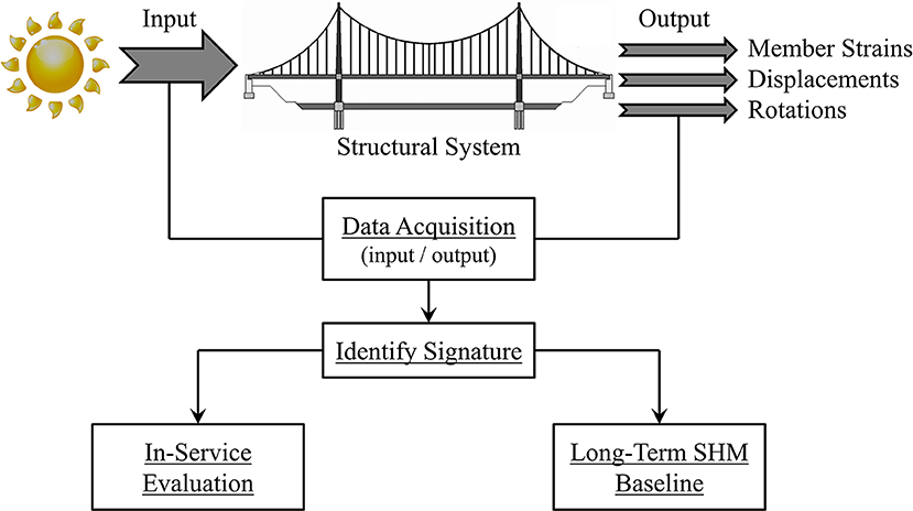
Figure 1. Temperature-driven bridge evaluation and monitoring approach.

Prior to presenting the research concepts and findings, background on thermal behavior of structural systems is discussed. The intent is to show the direct correlation between support stiffness and thermal member forces. In addition, the two different components of displacement (restrained and unrestrained) are to be clearly defined. To easily convey this behavior, consider a simple beam with a flexible longitudinal support at one end (Figure 2A). To determine the stress resulting from a uniform temperature change (ΔT) a statically indeterminate problem results. The solution can be obtained using superposition. The spring is removed and then applied as the redundant reaction. First, consider the member without the spring support (Figure 2B). The unrestrained deformation (δ_T) can be calculated as show in Equation (1) (corresponding to Figure 2C), where α and L are the coefficient of thermal expansion and member length, respectively.

$\begin{array}{ll}{\delta }_T=\alpha (\Delta T)L& (1)\end{array}$

The redundant force provided by the spring (F_s) is applied and the corresponding deformations can be identified (Figure 2D). This spring force is equal to the spring stiffness (k_s) multiplied by the unrestrained deformation (δ_U). The restrained deformation (δ_R) can be calculated from Equation (2), where A_m and E are the cross-sectional area of the member and modulus of elasticity, respectively.

$\begin{array}{ll}{\delta }_R=\frac{F_{S}L}{A_{m}E}& (2)\end{array}$

From Figure 2D, the portion of deformation that produces stress and strain can be observed. The unrestrained deformation (δ_U) produces strain without stress. However, the restrained deformation (δ_R) produces stress without strain. Therefore, the resulting thermal stress (σ_T) can be calculated from Equation (3) with ε_m representing the mechanical (or restrained) strain. Note the spring force and resulting axial stress is compressive for a positive ΔT (tensile for a negative ΔT).

$\begin{array}{ll}{\sigma }_T=E{\epsilon }_m=\frac{F_s}{A_m}& (3)\end{array}$

The study presented herein builds on these fundamental relationships to develop and implement several evaluation and monitoring methods focused on bridge bearings.

FIGURE 2

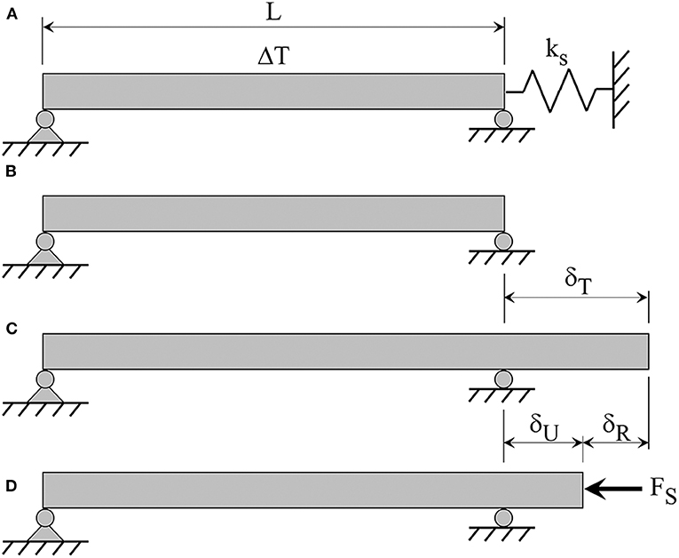
Figure 2. (A) simple span beam with a longitudinal spring, (B) beam without spring support, (C) total deformation due to uniform temperature change, and (D) restrained deformation due to spring force (shown in the negative direction).

Force Equilibrium Concept

Measurements can be taken at appropriate locations on a structure such that equilibrium can be used to evaluate and monitor bridge bearings (Yarnold and Dubbs, 2015). The overall concept is to measure the change in deformations of the members framing into the bearing, which can be used to back-calculate the change in member forces. The horizontal components of these member forces are then used with force equilibrium to identify the restraining force of the bearings. This restraining force can be compared to the original design drawings (if available) or reasonable estimates based on the structure.

To apply this method the appropriate sensing technology and instrumentation setup will depend on a number of factors. Stable sensing technology must be used. Measurements cannot drift over time so that adequate data sets are acquired (typically weeks to months). In addition, the equipment must be durable to withstand environmental effects and record reliable information. Fiber optic or vibrating wire sensors are adequate alternatives (Zalt et al., 2007).

The instrumentation setup must be able to obtain measurements that allow for back-calculation of the change in member forces. Typically, member deformations are measured using strain gages along with thermistors for temperature readings. The configuration of the sensors should allow for a free-body slice of the structure. Figure 3 illustrates general alternatives for two common bridge types (girder and truss). In Figure 3A, the intent is to measure the vertical strain profile and temperature gradient near the support of a girder bridge. Therefore, the induced axial deformation and curvature can be captured. As a result, the extent of any restrained translation and/or rotation can be obtained. For primarily axial members, such as those within trusses, a setup like that shown in Figure 3B is recommended.

FIGURE 3

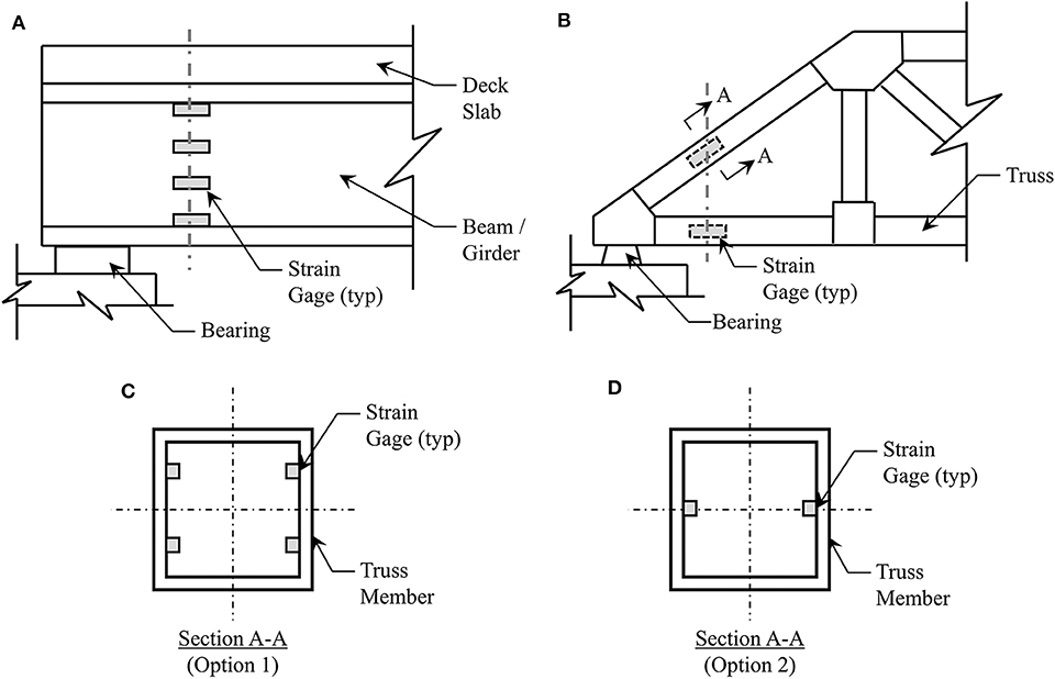
Figure 3. Free-body slice general illustrations for (A) Girder bridges or (B) Truss bridges and the potential sensor cross-section layouts for a truss member using a (C) detailed option and (D) less refined option.

The number of sensors per member cross-section is critical. Local member level gradients can be induced in the bridge members. It is recommended to provide four sensors, as shown in Figure 3C, to capture bending of the member in both directions. This information may not be required in all studies. However, one additional advantage is the redundancy of the measurements in that member allowing for easier data interpretation in the event one sensor is performing inadequately. If resources cannot support four sensor per member-cross section, then at a minimum two sensors, as shown in Figure 3D, should be provided. This setup allows for the capture of bending in one direction. Nonetheless, with the sensors placed at the neutral axis the measurements will not be affected for bending in the other direction. In either setup, the measurements can be averaged to identify the change in member axial component.

Thermoelasticity Concept

For expansion bearings a method is presented that uses the fundamentals of thermoelasticity. The overall concept is to measure temperature changes along with the corresponding longitudinal bearing movements. The movement of expansion bearings should correlate with temperature change. Therefore, measurement of the longitudinal movement of the bearings along with the ambient temperature provides the input-output relationship needed to compare the theoretical movement with reality.

The theoretical movement of bridge expansion bearings (δ_T) can be calculated from Equation (1). Rearranging terms produces Equation (4). The left side of the equation is field identified and compared to the right side, which is the product of a material property and a geometric property.

$\begin{array}{ll}{\delta }_T/\Delta T=\alpha ·L& (4)\end{array}$

The coefficient of thermal expansion (α) for steel and concrete is well-understood. In cases where this parameter is uncertain, material property testing can be performed to determine precise values. The unrestrained length of the bridge (L) is typically identified from the layout of the structure. The confidence is further improved by measuring movement at multiple locations. For example, consider a two-span continuous bridge with a fixed center pier and expansion abutments. The thermal neutral point (location where no temperature-induced movement occurs) should be at the pier, if all movement systems are functioning. Measurement of the movement at both ends of the bridge (as opposed to just one end) allows for more accurate identification of the thermal neutral point and resulting L values.

Non-physics Based Long-Term Bearing Monitoring for Damage Detection

As mentioned earlier, to achieve the four levels of SHM, a reliable baseline must be established to track “normal” behavior with time. This baseline can then be used for detection of anomalies, which are potentially as a result of structural damage. Identifying a sound baseline can be complex due to the highly non-linear behavior of constructed bridge systems. As a result, many non-physics based approaches have been used for monitoring bridges. The method for bearing assessment presented herein utilizes artificial neural networks (ANNs); however, many other algorithms could be applied.

Background of Bridge Monitoring using ANNs

ANNs are computing systems that emulate the information processing within the human brain. The primary components of ANNs are the processing elements (referred to as neurons) and the interconnection between these neurons. These connections have different strengths called weights, which are obtained through adaptive learning. This is achieved through an iterative input-output mapping process (Haykin, 1999). During this learning process, the weighted connections between neurons are modified by using optimization algorithms according to specific properties of the learning scheme. This allows ANNs the capability to model complex input-output functional relationships with general non-linear mapping capacity.

Researchers have investigated the use of ANNs for monitoring and damage detection of bridges. Earlier work performed by Pandey and Barai (1995) included numerical simulation studies of a simple truss bridge (Pandey and Barai, 1995). Damage scenarios included members simulated with a reduction in stiffness. Further numerical simulation studies of damage to truss joints (Mehrjoo et al., 2008) along with beam and frame structures (Zhao et al., 1998) using ANNs have been conducted. In these studies, the primary parameters used for damage detection were modal properties (frequencies and mode shapes). These studies did not include environmental effects. Recent research has focused on compensation of environmental effects using ANNs. The focus has been on the relationship between temperature and modal parameters (Ko and Ni, 2005; Li et al., 2010; Zhou et al., 2011). Kostić and Gül (2017) developed a generalized framework for damage assessment accounting for temperature effects by using output-only vibration and temperature data using ANNs (Kostić and Gül, 2017).

ANN SHM Baseline Concept

The chosen approach for bearing monitoring was to train an ANN using local temperature changes as the input layer along with global structural deformations (longitudinal displacement) as the output layers (Figure 4A). Supervised neural networks can be trained to produce desired outputs in response to sample inputs, making them particularly well-suited for modeling and controlling dynamic systems and predicting future events. The case study (presented in the following section) utilizes a dynamic time series analysis with a non-linear autoregressive (NARX) network. This allows for the prediction of a time series y(t) from past values of itself (d) and from another time series x(t). Figure 4B graphically illustrates the general NARX model.

FIGURE 4

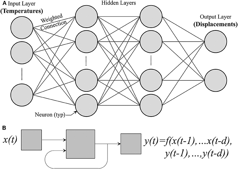
Figure 4. (A) Illustration of the multi-layer neural network and (B) illustration of the NARX model.

Once the ANN is trained, it can be used to predict future behavior (displacements in this case). These predictions can be compared with future measured values to identify anomalies. A damage index (DI) can be defined for automated detection. A basic expression is presented in Equation (5), where y_P(t) and y_M(t) are the ANN predicted and measured results at each time step, respectively.

$\begin{array}{ll}DI(t)={|y}_P(t)-y_M(t)|& (5)\end{array}$

There are benefits for this overall method. One benefit is the ability to readily obtain the information required to train the ANN and then compare with future measurements. Thermal “loads” can be the most significant service level demands a bridge experiences. Therefore, the responses of the structure can be accurately measured. However, one of the biggest challenges with these thermal measurements is that they can be highly non-linear and difficult to predict. This is an advantage of using machine-learning algorithms such as ANNs, since they have the capability to “learn” complex non-linear behavior.

Case Study Bridge

Hernando Desoto Bridge

The Hernando Desoto (HD) Bridge was utilized for the case study. The main section of the structure is a 548 m long, two-span, steel through arch bridge. Originally built in 1973, the HD Bridge is located in Tennessee, USA and carries Interstate 40 over the Mississippi River connecting Memphis, Tennessee to West Memphis, Arkansas. The structure supports six lanes of traffic with an overall width of 28 m and is a critical structure for the region. Figure 5 shows the main section of the structure and includes the pier labels.

FIGURE 5

Figure 5. Hernando Desoto (HD) bridge main spans (with Pier labels).

In 2000, the Tennessee Department of Transportation (TDOT) partnered with the Arkansas State Highway and Transportation Department (AHTD) to retrofit the bridge for a seismic event due to the New Madrid Fault system. The HD Bridge lies on the southeastern end of the New Madrid Seismic Zone, which is the most active seismic zone in the Central United States. The seismic retrofit protects the bridge from earthquakes with a moment magnitude of up to 7.7. One of the critical aspects of the retrofit was bearing system replacement with friction-pendulum isolation bearings. These friction pendulum bearings lengthen the natural period of the structure to help isolate the superstructure during any ground acceleration and dampen the lateral forces created by an earthquake. Due to the significant role the bearings have on the structure's seismic performance (and serviceability under thermal variations), significant time and research was conducted to evaluate the current behavior along with potential baselines for long-term monitoring.

Case Study SHM System

An SHM system was installed along the HD Bridge to provide TDOT with information for proactively maintaining the structure along with actionable information after a seismic event. Therefore, three main systems were installed. The first system is a vibration-based seismic monitoring program maintained by the University of Memphis, which includes a network of accelerometers at 36 locations along the structure (Steiner et al., 2006). The second system is a trigger-based non-contact displacement monitoring system that will capture the movement of the bearings in the event of seismic ground motion (Yarnold et al., 2017). The third system is a quasi-static setup that measures slow-speed strains of the members framing into the bearings, the longitudinal movement of the bearings, and the temperature changes. This quasi-static setup is the only portion of the SHM system used for the case study and, as a result, is the only system discussed further.

The instrumentation for the third system is concentrated at Pier A (west end) and Pier C (east end) of the double arch spans. The setup is the same at each location. Figure 6 graphically illustrates the setup at Pier A and Pier C. Note that access to the inside of the box-shaped members was restricted so the sensors were mounted to the outer face, but along the inside (or roadway side) of the member to avoid direct solar radiation effects.

FIGURE 6

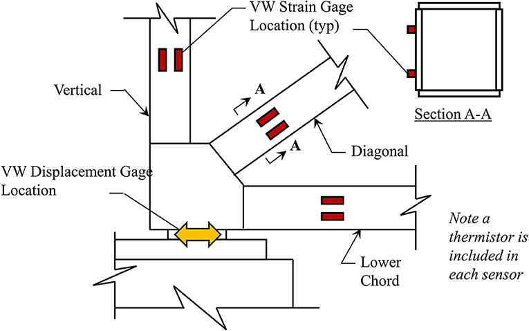
Figure 6. General instrumentation layout at Pier A (Pier C similar).

Vibrating wire (VW) sensing technology is utilized for the quasi-static system. Geokon Model 4420 sensors were selected (including internal thermistors) to measure the longitudinal displacements and temperatures (Figure 7). Geokon Model 4000 strain gages were selected (including internal thermistors) for measuring the member strains and temperatures. For all sensors, a relatively fast sampling rate (for thermal monitoring) of once every 5 min was chosen and then smoothed using a 25-min moving average during the future data processing stage. This helps remove any isolated influence of heavy traffic response, which is relatively small for a structure of this scale.

FIGURE 7

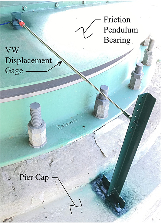
Figure 7. Longitudinal displacement measurement setup.

The data acquisition system for the project is from Campbell Scientific (CR1000) and is located at Pier A. The data from Pier C is collected and periodically sent to Pier A through a radio. At select time intervals, radio interference disrupts the data transfer and not all of the Pier C data is collected. Solutions to correct this issue were explored but due to budget and access issues, it was decided to proceed since the majority of the data (>75%) is being transferred. A cellular modem is also located at Pier A allowing the data to be wirelessly accessible offsite. Significant internal memory and battery backup power is included in the event communication and power are lost.

Installation of the SHM system was completed in 5 days with the last day designated for quality controls checks. Throughout the installation, TDOT provided lane closures to allow for the use of their Aspen A-62 snooper truck for strain gage attachment. These gages were epoxy mounted to the member surfaces. The VW displacement gages were mounted to the surface of the bearings and attached to a vertical bracket that was anchored to the pier cap (Figure 7). Once all the sensors were attached, cabling was performed for connection to the data acquisition system, which was housed in a weatherproof enclosure at the center of the pier cap. Further information regarding the SHM system itself can be found under Yarnold et al. (2017).

In-Service Bearing Evaluation

Force Equilibrium Method Results

The force equilibrium approach was applied for the case study bridge with the installation setup shown in Figure 6. The HD Bridge bearing mechanism is intended to behave in a non-linear cyclic pattern under service loads since it is a friction-based system. Essentially the bearings do not move until the static friction is overcome. Therefore, in the morning when the structure begins to heat up, the bearing is in the “stick” position until a temperature is reached which exerts a sufficient horizontal force. The bearing then “slips” and continues to move until the structure starts to cool. The movement in the other direction during cooling works in the same manner. This mechanism provides a unique signature for the structure that can be tracked with time. Figure 8 illustrates the typical bearing displacement vs. temperature relationship for 1 day of SHM data at Pier A. Note that this behavior is consistent with other friction-based bearing systems (Yarnold et al., 2015).

FIGURE 8

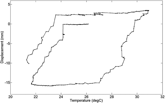
Figure 8. Example “stick-slip” behavior at the Pier A bearings.

The short-term data was processed to identify the “stick” subsets of response. For each of these time windows the change in mechanical strains measured in each arch member were collected. The strains were averaged, for each member, to obtain the axial components. Then the axial mechanical strains (ε_m) were converted to axial forces (F) using Equation (6), which is simply Equation (3) reordered.

$\begin{array}{ll}F=E·{\epsilon }_m·A_M& (6)\end{array}$

This process allowed for identification of the axial forces for each arch member framing into the bearings as shown in Figure 9.

FIGURE 9

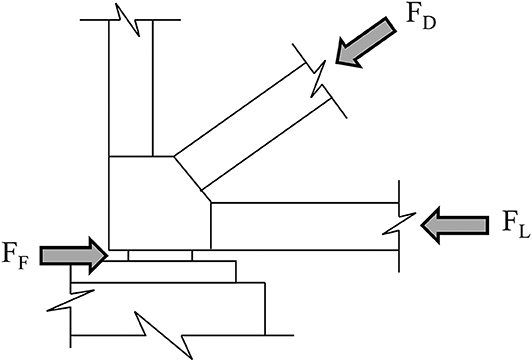
Figure 9. Free-body diagram at the arch bearings.

Horizontal equilibrium was then used to determine the static frictional force (F_F) (Equation 7).

$\begin{array}{ll}{F}_F=F_L+F_{D·}cos(\theta )& (7)\end{array}$

Once this frictional force was obtained for each “stick” period it was divided by the dead load reaction (provided by TDOT) to obtain the coefficient of friction.

Pier A and Pier C were evaluated separately. Pier A was evaluated first, which included the analysis of 24 “stick” periods for both the upstream (US) and downstream (DS) bearings. Table 1 shows a summary of the static frictional force results. The mean frictional force was slightly higher (8%) for the downstream bearing along with a higher standard deviation. The resulting mean coefficients of friction for the upstream and downstream bearings were the same or below the design (installation) value of 0.06. Table 1 also provides a summary of the Pier A coefficient of friction results, which are still within the original design specifications.

TABLE 1

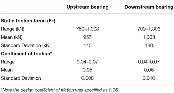
Table 1. Pier A static friction results.

It was intended to repeat the analysis for the bearings at Pier C. The arch bearings and installation setup at Pier C are identical to those at Pier A. However, the measured data is very different in nature. The order of magnitude of the displacements is much lower. During the first month of recording, virtually no appreciable displacements were observed. It was initially assumed that the bearings at each end experience similar movement since the two-span arch superstructure is symmetric.

An extensive assessment was conducted after reviewing the first month of Pier C data. First, data quality was evaluated to ensure the measurements were accurate. Then, an investigation was performed to ensure the Pier C bearings were not “frozen.” This was ruled out due to the minimal mechanical strains in the arch members framing into the bearings. Therefore, the resulting theory is that substructure movement is occurring (illustrated in Figure 10). The supporting piers are relatively flexible. In addition, the approach structures at each end of the arch spans are not symmetric superstructure types and have different bearing types. Therefore, the restoring longitudinal force provided by the approach at Pier C is much less than at Pier A. As a result, in many situations it is easier for Pier C to flex and/or rotate than it is for static friction to be overcome in the bearings. The result of this phenomenon is highly non-linear bearing longitudinal displacement at Pier C. Further evaluation concluded that this behavior is acceptable and is considered “normal” for this particular structure. Note that movement of Pier A is also possible. Though the data suggests it is relatively small.

FIGURE 10

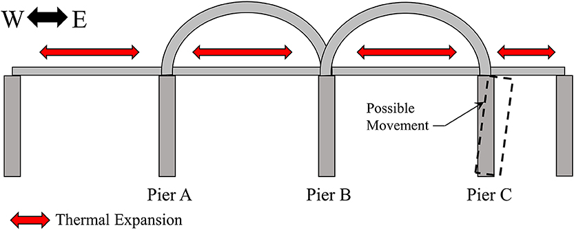
Figure 10. Illustration of the Pier C substructure movement.

Due to the non-linear response at Pier C it was concluded the force equilibrium approach could not be applied. The isolation of “stick” periods was inaccurate, which produced unreliable results. Further measurements of the Pier C global movement/rotation would be required. This clearly illustrates a limitation of the method and the challenges associated with long-term monitoring.

Thermoelasticity Method Results

The thermoelasticity approach was also applied for the case study bridge. This was a challenge due to the non-linear behavior. However, the long-term data sets were approximated as a linear relationship. Ten months of average displacement vs. average change in temperature data was used to identify the current relationship. Another technique was to only utilize evening data, minimizing thermal gradient effects, to capture near steady-state response. This technique was considered sufficient through analysis of the temperature data sets, which illustrated minimal evening differential between the 16 measurements. In addition, a comparison to a local weather station was performed. It should be noted that some studies (particularly of concrete structures) have shown this technique to not be valid (Reilly et al., 2016).

Pier A was evaluated and found <2% difference between the theoretical and actual movement. The Pier A upstream (US) and downstream (DS) bearings exhibited a 3.15 and 3.19 mm/°C, respectively. Figure 11 illustrates evening data over 10 months along with a linear best-fit line. The theoretical behavior was calculated as 3.21 mm/°C. Overall, the Pier A results from the force equilibrium and the thermoelasticity approaches indicate adequate functionality of the bearings.

FIGURE 11

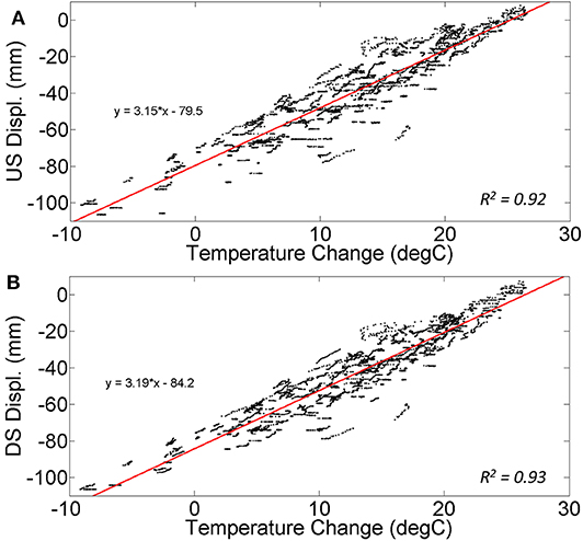
Figure 11. Displacement vs. temperature relationship over 10 months at (A) Pier A upstream and (B) Pier A downstream.

Pier C could not be adequately evaluated using the thermoelasticity approach for similar reasons mentioned in the prior section. The movement of Pier C itself made it unreliable to use this method without further measurements of the Pier C global movement.

Long-Term Bearing Monitoring

ANN SHM Baseline Assessment

Baselines for long-term monitoring and future damage detection of the HD Bridge bearings were investigated using dynamic time series analyses, which was performed utilizing the Matlab neural network toolbox. The time series tool was chosen for the capabilities to solve dynamic modeling and prediction problems. As mentioned earlier, non-linear autoregressive exogenous models (NARX) were utilized. This allowed for the prediction of a time series y(t) from past values of itself (d) and from another time series x(t) (Figure 4B).

To train the ANN, the input/output thermal relationship was utilized. The input to the system were the time series temperature values for all of the 16 sensor locations. These 16 sensors include the 12 member cross-sections instrumented. Figure 6 illustrates the three arch members instrumented at each of the four corners of the bridge. The remaining four temperature sensors were located at each of the four displacement sensors. This provided an overall distribution of temperature measurements.

The output was the corresponding longitudinal displacements at each of the four bearings. The network was set with 10 hidden neurons and 2 time delays. Figure 12 provides the neural network diagram (w indicates weight factor and b the bias). The Levenberg-Marquardt method for algorithm training was selected where a performance index is used to minimize the sum of squares of errors, with optimizing parameter vectors. Note the number of hidden neurons and time delays were selected from a sensitivity study utilizing the training error data. Less hidden neurons could have been utilized, however, processing time was not an issues so it was not reduced.

FIGURE 12

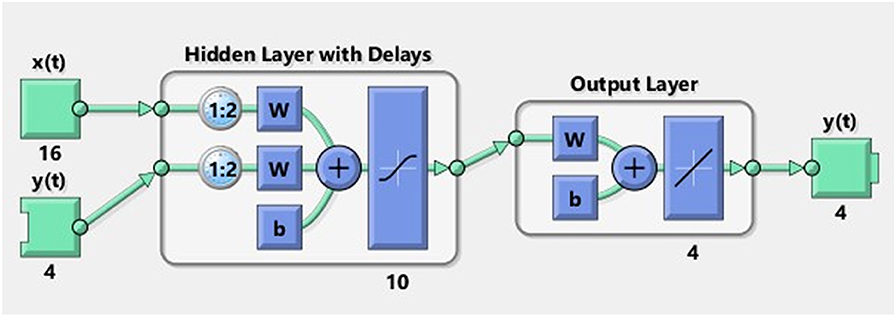
Figure 12. Neural network diagram for the case study.

Approximately 10 months of data was used for this study with 85% selected for training. The training results were excellent with very low mean square errors (9.2 × 10⁻⁶) along with near one regression R values (correlation between the outputs and targets). The remaining 15% was utilized for the evaluation of the baseline for potential bearing damage detection. The more accurate prediction capabilities could indicate higher probability for identifying anomalies.

Prediction Study

A comparison of the predicted data verses the measured SHM data using ANNs is presented in Figures 13A, 14A (time axis denoted by the measurement record number). These figures provide the upstream displacements at Pier A and Pier C, respectively. The downstream results are not shown, but are very similar. As mentioned earlier, radio interference disrupted data transfer causing some data to be lost. This is the reason for the gaps in the measured data presented in the figures. Notice that despite gaps in the data the baseline still accurately predicts the response.

FIGURE 13

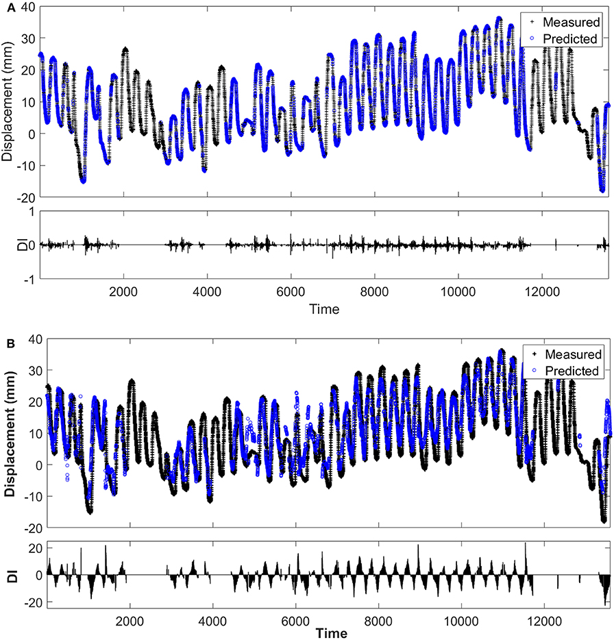
Figure 13. (A) Pier A measured and ANN predicted results and (B) Pier A measured and conventional SHM baseline results.

FIGURE 14

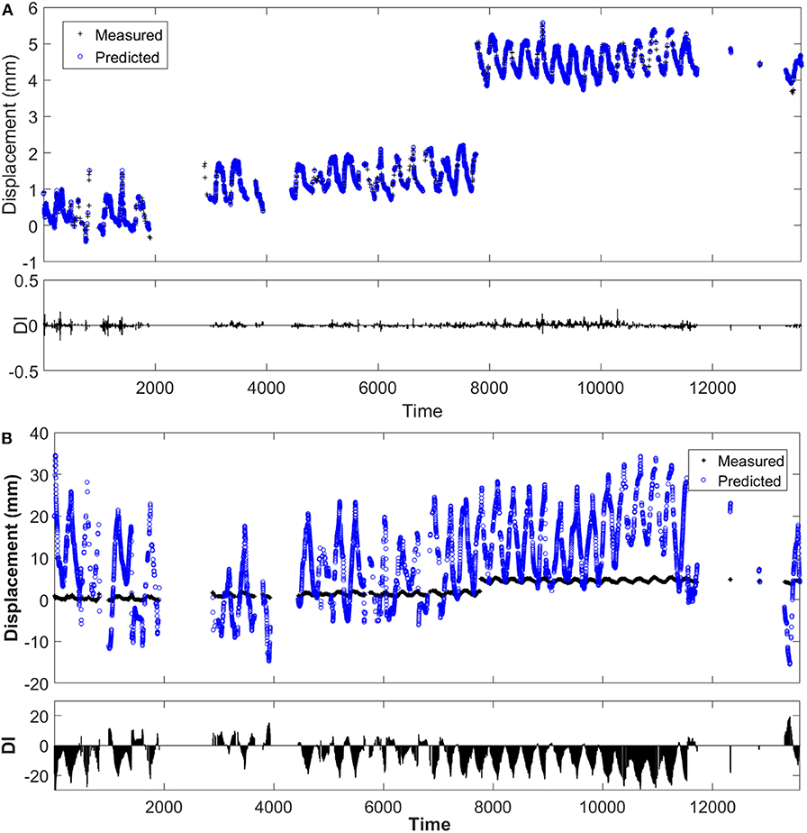
Figure 14. (A) Pier C measured and ANN predicted results and (B) Pier C measured and conventional SHM baseline results.

To quantitatively evaluate the potential for anomaly detection the root mean square error (RMSE) was calculated. The RMSE for Pier A upstream and downstream bearings were both 0.06 mm. The RMSE for Pier C upstream and downstream bearings were both 0.04 mm. To adequately identify damage the change in baseline must be well outside the typical variability. Note that the specific threshold values should be defined after rigorous analysis.

Comparison Study

To further assess the capabilities of the ANN SHM baseline, a comparison was performed with a conventional service level SHM baseline for bearings. One conventional technique for long-term tracking of bearing movement is to utilize thermoelasticity similar to that shown earlier. Equation (4) can be rearranged to predict the displacements (δ) based on the measured temperature changes (ΔT) along with an estimated coefficient of thermal expansion (α) and unrestrained length (L). For the case study bridge α and L were taken as 1.17e-5 mm/mm°C (provided by the bridge owner) and 274 m (assuming a thermal neutral point at the center pier), respectively.

Predicted bearing movements were developed using the conventional technique for the last 15% of measured SHM data and compare to the ANN predictions. Localized temperatures were used at each of the four bearing locations. A comparison of the Pier A upstream results is provided in Figure 13B. It can be seen that the general time history trends was matched. However, comparing the DI values for the conventional technique with the ANN baseline (shown in Figure 13A) quantitatively concludes that the ANN baseline has significantly more accurate prediction capabilities. For example, the DI range for the conventional method was ±23 mm where the ANN baseline was only ±0.4 mm. The results for the Pier A downstream bearing were consistent with the upstream results.

A comparison of the Pier C results was also performed. Figure 14B provides the upstream conventional technique predictions compared with those measured. In this case, even more severe discrepancy was found. The order of magnitude is substantially different. As mentioned earlier, it was identified in the evaluation that Pier C itself is moving. Therefore, it was not surprising that the conventional baseline provided poor prediction. Essentially a mechanism was not being accounted for. The purpose of showing the conventional technique for Pier C is to further illustrate the necessity in this case study to utilize a non-physics based baseline (such as ANNs) and their drastic improvement over conventional approaches (shown in Figure 14A).

Conclusions

Bridge bearing mechanisms can be evaluated in-service and/or monitored long-term using quasi-static measurements. This was researched though a field case study of a long-span arch bridge with friction-pendulum isolation bearings. The specific case study findings for both evaluation and monitoring are summarized below. In addition, general contributions of the research are included.

In-Service Evaluation

Physics-based methods were evaluated to assess the current bearing condition. This included two general approaches that utilized force equilibrium and thermoelasticity. The equilibrium methodology was able to identify the friction force both Pier A bearings. They were found to still be within 8% of their original design specified values and therefore considered to be functioning properly. Conversely, the frictional force could not be identified at Pier C due to the highly non-linear behavior exhibited. This behavior was tracked to unique pier movement. In general, the equilibrium methodology can be considered for evaluation of bearings that behave in a linear or bi-linear manner. However, this method should not be applied for highly non-linear situations (such as the bearing at Pier C in the case study).

The thermoelasticity methodology produced consistent results with the force equilibrium approach. The bearings at Pier A were evaluated and exhibited <2% difference between the theoretical and actual movement. Again, the Pier C highly non-linear bearing behavior did not allow for evaluation.

Overall, the research contribution to the state-of-the-art is two valid methods for in-service bearing evaluation. Currently, the literature is limited on accurate in-service evaluation techniques, particularly for friction-based systems. The presented research illustrates the methods, evaluates them through a case study, and provides the benefits and limitations of each.

Long-Term Monitoring

The limitations found with the in-service bearing evaluations (due to highly non-linear behavior) led the research team to explore non-physics-based methods to establish a baseline for long-term monitoring. Artificial neural networks (ANNs) were utilized with success. This was determined through comparison with a conventional bearing monitoring baseline (using thermoelasticity). The results from the Pier A bearings showed a conventional damage index range (prediction capability) of ±23 mm, whereas the ANN found only ±0.4 mm. At Pier C, an even larger disparity was found. In general, the study concluded that the prediction capabilities of the ANN were excellent. The comparative study between a conventional baseline with the ANN baseline showed significantly higher potential for bearing damage detection.

A unique aspect of the study was that an ANN was trained using thermal “loads” to predict longitudinal displacement of the bearings. Thermal demands are commonly the largest service level response that can be measured and are sensitive to structural changes. The presented research illustrates a viable method that was evaluated through a challenging case study.

Data Availability Statement

The datasets generated for this study are available on request to the corresponding author.

Author Contributions

All authors have contributed to the contents within this paper. The primary research was conducted by JA during his graduate studies. MY was JA's advisor and contributed to this study through the review of each research stage along with assisting the field installation.

Funding

This material is partly based upon work supported by the NSF under Grant No. CMMI-1434373.

Conflict of Interest

The authors declare that the research was conducted in the absence of any commercial or financial relationships that could be construed as a potential conflict of interest.

Acknowledgments

The authors would like to thank the Tennessee Department of Transportation for their funding of this project. The authors would also like to thank the University of Memphis for their support and coordination of the field installation. In addition, the authors would like to thank the National Science Foundation (NSF). Any opinions, findings, and conclusions or recommendations expressed in this material are those of the authors and do not necessarily reflect the views of NSF.

References

Brownjohn, J. M. W., Magalhaes, F., Caetano, E., and Cunha, A. (2010). Ambient vibration re-testing and operational modal analysis of the Humber Bridge. Eng. Struct. 32, 2003–2018. doi: 10.1016/j.engstruct.2010.02.034

CrossRef Full Text | Google Scholar

Brownjohn, J. W., Stefano, A., Xu, Y.-L., Wenzel, H., and Aktan, A. E. (2011). Vibration-based monitoring of civil infrastructure: challenges and successes. J. Civil Struct. Health Monitor. 1, 79–95. doi: 10.1007/s13349-011-0009-5

CrossRef Full Text | Google Scholar

Cao, Y., Yim, J., Zhao, Y., and Wang, M. L. (2011). Temperature effects on cable stayed bridge using health monitoring system: a case study. Struct. Health Monitor. 10, 523–537. doi: 10.1177/1475921710388970

CrossRef Full Text | Google Scholar

Catbas, F. N., Ciloglu, S. K., Hasancebi, O., Grimmelsman, K., and Aktan, A. E. (2007). Limitations in structural identification of large constructed structures. J. Struct. Eng. 133, 1051–1066. doi: 10.1061/(ASCE)0733-9445(2007)133:8(1051)

CrossRef Full Text | Google Scholar

Cornwell, P., Farrar, C. R., Doebling, S. W., and Sohn, H. (1999). Environmental variability of modal properties. Exp. Tech. 23, 45–48. doi: 10.1111/j.1747-1567.1999.tb01320.x

CrossRef Full Text | Google Scholar

Cruz, P. J. S., and Salgado, R. (2009). Performance of vibration-based damage detection methods in bridges. Comput. Aided Civil Infrastruct. Eng. 24, 62–79. doi: 10.1111/j.1467-8667.2008.00546.x

CrossRef Full Text | Google Scholar

De Roeck, G. (2003). The state-of-the-art of damage detection by vibration monitoring: the SIMCES experience. J. Struct. Control 10, 127–134. doi: 10.1002/stc.20

CrossRef Full Text | Google Scholar

Dubbs, N., Moon, F., and Aktan, A. E. (2010). Design and Implementation of Load Cells to Measure Dead and Live Load Effects in an Aged Long Span Bridge. Philadelphia, PA: International Association for Bridge Management and Safety.

Google Scholar

FHWA (2001). 23 CFR Part 650. FHWA Docket No. FHWA−2001–8954. National Bridge Inspection Standards. Washington, DC. RIN 2125–AE86.

Fujino, Y., Abe, M., Shibuya, H., Yanagihara, M., Sato, M., Nakamura, S.-I., et al. (2000). Forced and ambient vibration tests and vibration monitoring of hakucho suspension bridge. Transport. Res. Rec. 1696, 57–63. doi: 10.3141/1696-43

CrossRef Full Text | Google Scholar

Gangone, M. V., Whelan, M. J., and Janoyan, K. D. (2011). Wireless monitoring of a multispan bridge superstructure for diagnostic load testing and system identification. Comput. Aided Civil Infrastruct. Eng. 26, 560–579. doi: 10.1111/j.1467-8667.2010.00711.x

CrossRef Full Text | Google Scholar

Gaoxin, W., and Youliang, D. (2015). Research on monitoring temperature difference from cross sections of steel truss arch girder of Dashengguan Yangtze Bridge. Int. J. Steel Struct. 15, 647–660. doi: 10.1007/s13296-015-9011-9

CrossRef Full Text | Google Scholar

Haykin, S. (1999). Introduction. Neural Networks: A Comprehensive Foundation. Upper Saddle River, NJ: Prentice-Hall.

Google Scholar

He, X., Moaveni, B., Conte, J. P., Elgamal, A., and Masri, S. F. (2008). Modal identification study of vincent thomas bridge using simulated wind-induced ambient vibration data. Comput. Aided Civil Infrastruct. Eng. 23, 373–388. doi: 10.1111/j.1467-8667.2008.00544.x

CrossRef Full Text | Google Scholar

Ko, J. M., and Ni, Y. Q. (2005). Technology developments in structural health monitoring of large-scale bridges. Eng. Struct. 27, 1715–1725. doi: 10.1016/j.engstruct.2005.02.021

CrossRef Full Text | Google Scholar

Ko, J. M., Zhou, H. F., and Ni, Y. Q. (2008). “A data processing and analysis system for the instrumented suspension Jiangyin Bridge,” in World Forum on Smart Materials and Smart Structures Technology (London: CRC Press).

Google Scholar

Kostić, B., and Gül, M. (2017). Vibration-based damage detection of bridges under varying temperature effects using time-series analysis and artificial neural networks. J. Bridge Eng. 22:04017065. doi: 10.1061/(ASCE)BE.1943-5592.0001085

CrossRef Full Text | Google Scholar

Kromanis, R., and Kripakaran, P. (2016). SHM of bridges: characterising thermal response and detecting anomaly events using a temperature-based measurement interpretation approach. J. Civil Struct. Health Monitor. 6, 237–254. doi: 10.1007/s13349-016-0161-z

CrossRef Full Text | Google Scholar

Kromanis, R., Kripakaran, P., and Harvey, B. (2015). Long-term structural health monitoring of the Cleddau bridge: evaluation of quasi-static temperature effects on bearing movements. Struct Infrastruct. Eng. 12, 1–14. doi: 10.1080/15732479.2015.1117113

CrossRef Full Text | Google Scholar

Kulprapha, N., and Warnitchai, P. (2012). Structural health monitoring of continuous prestressed concrete bridges using ambient thermal responses. Eng. Struct. 40, 20–38. doi: 10.1016/j.engstruct.2012.02.001

CrossRef Full Text | Google Scholar

LeDiourion, T., and Hovhanessian, G. (2005). “The health monitoring of Rion Antirion Bridge,” in IMACXXIII (Orlando, FL).

Li, H., Li, S., Ou, J., and Li, H. (2010). Modal identification of bridges under varying environmental conditions: temperature and wind effects. Struct. Control Health Monitor. 17, 495–512. doi: 10.1002/stc.319

CrossRef Full Text | Google Scholar

Li, H., Ou, J., Zhao, X., Zhou, W., Li, H., Zhou, Z., et al. (2006). Structural health monitoring system for the Shandong Binzhou Yellow River Highway Bridge. Comput. Aided Civil Infrastruct. Eng. 21, 306–317. doi: 10.1111/j.1467-8667.2006.00437.x

CrossRef Full Text | Google Scholar

McDonald, J., Heymsfield, E., and Avent, R. (2000). Slippage of neoprene bridge bearings. J. Bridge Eng. 5, 216–223. doi: 10.1061/(ASCE)1084-0702(2000)5:3(216)

CrossRef Full Text | Google Scholar

Mehrjoo, M., Khaji, N., Moharrami, H., and Bahreininejad, A. (2008). Damage detection of truss bridge joints using Artificial Neural Networks. Expert Syst. Appl. 35, 1122–1131. doi: 10.1016/j.eswa.2007.08.008

CrossRef Full Text | Google Scholar

Mosavi, A. A., Seracino, R., and Rizkalla, S. (2012). Effect of temperature on daily modal variability of a steel-concrete composite bridge. J. Bridge Eng. 17, 979–983. doi: 10.1061/(ASCE)BE.1943-5592.0000372

CrossRef Full Text | Google Scholar

Moser, P., and Moaveni, B. (2011). Environmental effects on the identified natural frequencies of the Dowling Hall Footbridge. Mech. Syst. Signal Process. 25, 2336–2357. doi: 10.1016/j.ymssp.2011.03.005

CrossRef Full Text | Google Scholar

Pandey, P. C., and Barai, S. V. (1995). Multilayer perceptron in damage detection of bridge structures. Comput. Struct. 54, 597–608. doi: 10.1016/0045-7949(94)00377-F

CrossRef Full Text | Google Scholar

Reilly, J., Abdel-Jaber, H., Yarnold, M., and Glisic, B. (2016). “Identification of steady-state uniform temperature distributions to facilitate a temperature driven method of structural health monitoring,” in Proceedings SPIE (Las Vegas, NV).

Google Scholar

Rytter, T. (1993). Vibration based inspection of civil engineering structure (PhD). Aalborg University, Aalborg, Denmark.

Google Scholar

Soyoz, S., and Feng, M. Q. (2009). Long-term monitoring and identification of bridge structural parameters. Comput. Aided Civil Infrastruct. Eng. 24, 82–92. doi: 10.1111/j.1467-8667.2008.00572.x

CrossRef Full Text | Google Scholar

Steiner, G., Withers, M., and Pezeshk, S. (2006). Seismic Instrumentation at the I-40 Hernando Desoto Bridge in Memphis. St. Louis, TN: Structures Congress.

Google Scholar

Wong, K. Y. (2010). “Structural health monitoring and safety evaluation of stonecutters bridge under the in-service condition,” in Bridge Maintenance, Safety, Management and Life-Cycle Optimization: IABMAS (Philadelphia, PA), 2641–2648.

Xia, Q., Cheng, Y., Zhang, J., and Zhu, F. (2017). In-service condition assessment of a long-span suspension bridge using temperature-induced strain data. J. Bridge Eng. 22:04016124. doi: 10.1061/(ASCE)BE.1943-5592.0001003

CrossRef Full Text | Google Scholar

Yang, D., Youliang, D., and Aiqun, L. (2010). Structural condition assessment of long-span suspension bridges using long-term monitoring data. Earthquake Eng. Eng. Vibrat. 9, 123–131. doi: 10.1007/s11803-010-9024-5

CrossRef Full Text | Google Scholar

Yarnold, M., Alexander, J., and Huff, T. (2017). “Structural health monitoring of the hernando desoto bridge,” in International Bridge Conference (National Harbor, MD).

Google Scholar

Yarnold, M., Murphy, B., Glisic, B., and Reilly, J. (2016). “Temperature-based evaluation and monitoring techniques for long-span steel bridges, in Proceedings from the Transportation Research Board (Washington, DC).

Google Scholar

Yarnold, M. T. (2013). Temperature-based structural identification and health monitoring for long-span bridges (Doctor of Philosophy). Drexel University, Philadelphia, United States.

Google Scholar

Yarnold, M. T., and Dubbs, D. C. (2015). Bearing assessment using periodic temperature-based measurements. Transport. Res. Rec. 2481, 115–123. doi: 10.3141/2481-15

CrossRef Full Text | Google Scholar

Yarnold, M. T., and Moon, F. L. (2015). Temperature-based structural health monitoring baseline for long-span bridges. Eng. Struct. 86, 157–167. doi: 10.1016/j.engstruct.2014.12.042

CrossRef Full Text | Google Scholar

Yarnold, M. T., Moon, F. L., and Aktan, A. E. (2015). Temperature-based structural identification of long-span bridges. J. Struct. Eng. 141:04015027-1–04015027-10. doi: 10.1061/(ASCE)ST.1943-541X.0001270

CrossRef Full Text | Google Scholar

Zalt, A., Meganathan, V., Yehia, S., Abudayyeh, O., and Abdel-Qader, I. (2007). “Evaluating sensors for bridge health monitoring,” in IEEE EIT (Chicago, IL).

Google Scholar

Zhao, J., Ivan, J. N., and DeWolf, J. T. (1998). Structural damage detection using artificial neural networks. J. Infrastruct. Syst. 4, 93–101. doi: 10.1061/(ASCE)1076-0342(1998)4:3(93)

CrossRef Full Text | Google Scholar

Zhou, H. F., Ni, Y. Q., and Ko, J. M. (2011). Eliminating temperature effect in vibration-based structural damage detection. J. Eng. Mech. 137, 785–796. doi: 10.1061/(ASCE)EM.1943-7889.0000273

CrossRef Full Text | Google Scholar

Zhu, Y., Fu, Y., Chen, W., Huang, S., and Bennett, K. D. (2003). “Health monitoring system for dafosi cable-stayed bridge,” in SPIE (San Diego).

Google Scholar