Probabilistic Design of Sustainable Reinforced Concrete Infrastructure Repairs Using SIPmath

1. Introduction

The design, construction, and operation of civil infrastructure that is more environmentally, socially, and economically responsible over its full life cycle from extraction of raw materials to end of life is increasingly desirable worldwide (Lepech, 2018). This can be seen emphasized in the United Nation's sustainability goals. The three design goals of improved environmental, social, and economic performance are commonly known as the “triple bottom line” of sustainability. As a critical set of systems that support quality of life and enable global development, while consuming vast amounts of material resources and energy, it is essential that civil infrastructure is designed according to these broad, long term design goals for the benefit of our planet and the current and future generations of humans, animals, and plants that will call it home. Currently, cement production results in 6–10% of total anthropogenic greenhouse gases (Scrivener et al., 2018). With a practical, easily implemented method for assessing the sustainability of new and current infrastructure, this impact can be managed and reduced.

While the goals of such sustainable design are well-intended, the creation and execution of civil infrastructure designs that are socially, environmentally, and economically sustainable is not functionally possible for current practitioners. This inability is due to a lack of quantitative targets for a “sustainable” design, quantitative metrics for measurement and comparison of designs, and a probabilistic-based design approach that is translatable to engineering practices that manage uncertainty in infrastructure design, construction, and use (Lepech, 2018). Current sustainable design approaches use a rubric to accumulate points, where in theory a higher score leads to a more sustainable building. The issue with this approach is the lack of quantitative, comparable metrics as well as unintended biases in weighting of rubric categories (Ehrenfeld, 2007). Further, current approaches do not allow for simple, straightforward comparisons between systemic and aleatory uncertainty in design, and the costs associated with reducing such uncertainties. This is in contrast to probabilistic structural design approaches that are the hallmark of modern civil engineering design around the world (e.g., AISC-LRFD in the US, ACI-318 in the US, Eurocode 2 in Europe).

Within civil engineering design probability is usually incorporated into codes to allow for consideration of uncertainty without having to directly apply probabilistic tools. A common example of this is the LRFD method, which applies factors to both the capacity and demand of a structural element. Though only deterministic values are considered in the engineering calculations of this method, these factors account for the uncertainty of each of the values. Additionally, it has been shown that when engineers are given a tool to quantify demand of an infrastructure project, they are much more likely to meet design targets (Russel-Smith et al., 2015). However, there are currently no tools to quantify the sustainability of an infrastructure project.

Along these lines, the design of sustainable rehabilitation of civil infrastructure proposed in this paper is based on the probabilistic framework for service life design proposed by the 2006 fib Model Code for Service Life Design of Reinforced Concrete (fib, 2006) and embodied in the fib 2010 Model Code (fib, 2010). This framework is implemented with an easy to use tool that removes the direct use of probabilistic methods from the calculations and allows for quick iterations of calculation. The purpose of this paper is to show a unique, practical method to use the framework introduced by Lepech et al. with SIPmath™ (Lepech et al., 2014). In section 2, this paper provides an overview of the framework for probabilistic design of sustainable reinforced concrete infrastructure repairs and presents the probabilistic design formulation, the novel application of SIPmath in native Excel^® to enable simple, straightforward design comparisons by practitioners. Section 3 discusses the results of a simplified case study of a reinforced concrete bridge exposed to spray from roadway deicing salts. Section 4 provides conclusions.

2. Methods

2.1. Framework for Probabilistic Design of Civil Infrastructure

Probabilistic design of sustainable civil infrastructure rehabilitations begins with measurement of the cumulative environmental, social, or economic impacts of a facility's repair and rehabilitation activities from initial construction up to the time of functional obsolescence. This is shown in Figure 1 (Lepech et al., 2013). Cumulative impact can be expressed as midpoint environmental indicators such as global warming potential (kg CO₂-equivalents), polluted water (L), solid waste (kg), or primary energy (MJ).

FIGURE 1

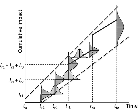
Figure 1. Probabilistic envelope of cumulative impacts of repairs and rehabilitations of civil infrastructure from initial construction (t₀) to functional obsolescence (t_fo) (Lepech et al., 2013).

As seen in Figure 1, the time at which any repair, j, is performed (t_rj) is probabilistically characterized based on reaching a service life limit state corresponding to an unacceptable reduction in a material's quality or structural performance. These distributions are shown as horizontal Gaussian distributions for illustration. The probabilistic time between repairs (t_rj+1−t_rj) is based on the chosen repair strategy, the quality of the repair work, the variable nature of exposure and load conditions, the limit state, etc. It should be noted that Figure 1 is a generalized graph of cumulative impact, including many possible scenarios. For example, a sloped line is shown between t_r3 and t_r4 to show the effects of cathodic protection between repairs.

The cumulative impact of the repair timeline is the sum of all impacts associated with a facility's repair and rehabilitation from initial construction up to the time of functional obsolescence. Metrics of environmental impact are based on globally accepted environmental impact assessment midpoint indicator protocols (e.g., TRACI in the US, ReCiPe in Europe), which can include climate change, acidification, land use, energy, and toxicity indicators. As also seen in Figure 1, the impact associated with each repair or rehabilitation action is probabilistic in nature (shown as vertical Gaussian distributions for illustration). The impact associated with a given repair action, i_rj, can vary due to uncertainty in the repair construction processes used, uncertainty in the supply chain of repair materials, uncertainty in the effects on infrastructure users (e.g., how many automobiles are disrupted by the repair construction), etc.

Combining the probabilistic models for both repair timeline (t_rj) and amount of impact (i_rj), a probabilistic envelope can be constructed for the entire infrastructure service life from the time of initial construction (t₀) to the time of functional obsolescence (t_fo). Based on the boundaries of this larger envelope (shown as dashes in Figure 1), an aggregated probabilistic envelope of cumulative environmental, social, or economic impact at any time, t, for the repaired structure can be calculated. This results in a probabilistic distribution of cumulative impact at a given point in the structure's lifespan.

This probabilistic distribution of impact can then be compared to a probabilistic distribution of sustainable design targets. Sustainable design targets are drawn from policy goals, which are derived from scientific, political, technological, or economic assessments of “sustainable development.” For example, design targets could be adopted from the Intergovernmental Panel on Climate Change's proposed reductions in global greenhouse gas emissions (IPCC, 2013). A broader set of sustainable design targets are discussed in Bakshi et al. (2015). With the goal of reducing impacts over time, an alternative (i.e., more sustainable) repair and rehabilitation scenario can be proposed. This probabilistic distribution of sustainable design targets can then be compared to the actual impact distribution at a given point in time to determine a probability of failure, the number of times the impact of the design exceeds the designated design targets.

The potential impact reduction using an alternative, more sustainable repair timeline vs. a status quo repair timeline can be estimated probabilistically at any time in the future. For instance, to achieve a safe, stabilized atmospheric carbon-equivalent concentration of 500–550 ppm, a 30–60% reduction in annual carbon-equivalent emissions is needed by Year 2050 (Year 2000 baseline) according to the UN Intergovernmental Panel on Climate Change (IPCC, 2013). Such reduction targets allow engineers to rationally design and probabilistically evaluate [through a probability of failure, P_f(t)], a cadre of infrastructure repair and rehabilitation timelines and technologies that meet proposed IPCC. Using this framework, engineers are incentivized to meet reduction targets at lowest economic cost, provided that the level of confidence that sustainability targets are met remains constant and acceptable. Tradeoffs between confidence levels (probabilities of failure) and cost can also be explicitly considered.

2.2. Probabilistic Sustainable Design Formulation in Excel Using SIPmath™

As seen from the orthogonal distributions in Figure 1, probabilistic sustainable design requires two distinct modeling components; (i) time-dependent modeling of material and structural deterioration, and (ii) cumulative environmental, social, and economic impacts of repair and rehabilitation activities. For a reinforced concrete structure undergoing a series of repairs over its lifetime, both of these components are described in the following sections. Also seen in Figure 1 is the interconnected nature of these two models, such that the design and completion of an individual repair activity heavily influences both the time until the next repair is needed along with the impacts associated with carrying out the repair activity. In reinforced concrete, this is seen through the variability in concrete depth. A larger concrete cover leads to an increased impact both in application and removal, but it also results in a longer time to repair.

2.2.1. Service Life Model

Service life models are used to quantify the performance of the structure over time. For demonstration purposes, a simple, probabilistic service life model for a reinforced concrete structure is adopted from the 2006 fib Model Code for Service Life Design of Reinforced Concrete (fib, 2006). This simple chloride-induced corrosion initiation (i.e., steel depassivation) model is convenient for demonstration of the SIPmath approach to performing sustainable design of civil infrastructure in Excel. Based on Fick's Second Law, all that is needed are probabilistic quantifications of the corrosion initiation limit state and a model of chloride-induced reinforcement corrosion progress as a function of time.

As proposed in the 2006 fib Model Code for Service Life Design of Reinforced Concrete (fib, 2006), the corrosion initiation limit state is defined by the chloride ion concentration at the location of the reinforcing steel reaching a critical concentration, as seen in (1).

$\begin{array}{ll}{C}_{crit}=C((x,t)=(d,t))& (1)\end{array}$

where, C_crit is the critical chloride concentration in weight % of cement, C(x, t) the chloride concentration in weight % of cement at time, t, at depth, x, from the concrete surface in meters, and d the concrete cover in meters.

The time dependent concentration of chlorides at depth, x, from the concrete surface is provided as (2) through (6).

$\begin{array}{ll}C((x,t)=(d,t))=C_0+(C_{s,\Delta x}-C_0)\lambda & (2)\end{array}$

$\begin{array}{ll}\lambda =1-erf\frac{d-\Delta x}{2\sqrt{D_{app,C}*t}}& (3)\end{array}$

$\begin{array}{ll}{D}_{app,C}=k_e*D_{RCM,0}*k_t*A(t)& (4)\end{array}$

$\begin{array}{ll}{k}_e=exp(b_e(\frac{1}{T_{ref}}-\frac{1}{T_{real}}))& (5)\end{array}$

$\begin{array}{ll}A(t)={(\frac{t_0}{t})}^a& (6)\end{array}$

where, C₀ is the initial chloride content of the concrete in weight % of cement, C_s,Δx the chloride content at a depth Δx and a certain point in time in weight % of cement, erf the error function, Δx the depth of concrete convection zone in meters, D_app,C the apparent chloride diffusion coefficient of the concrete in m²/year, D_RMC,0 the chloride migration coefficient in m²/year, k_e a dimensionless environmental transfer variable, b_e a regression variable in degrees K, T_ref a standard temperature in K, T_real the temperature of the reinforced concrete element or ambient air temperature in K, A(t) a dimensionless aging variable expressed as a function of time, t, t₀ a reference time in years, and a a dimensionless aging exponent. The values or distributions in (2) through (6) are provided in Table 1. The value for C_s,Δx and the mean and standard deviation for D_RMC,0 are determined using water to cement ratio.

TABLE 1

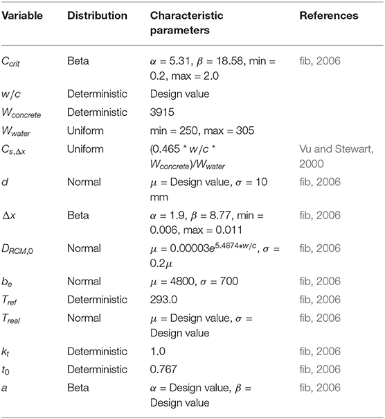
Table 1. Service life modeling variables, distributions, and characteristic parameters.

In order to compute the time to reach the critical chloride concentration at the reinforcement, the error function is modeled using an approximation by (Abramowitz and Stegun, 1983), shown in (7) and (8).

$\begin{array}{ll}erf=1-({\displaystyle \sum _{i=1}^5}(a_i{\xi }^i))e^{-x^2}& (7)\end{array}$

$\begin{array}{ll}\xi =\frac{1}{1+px}& (8)\end{array}$

where, p is equal to 0.3275911, a₁ is equal to 0.254829592, a₂ is equal to −0.284496736, a₃ is equal to 1.421413741, a₄ is equal to −1.453152027, and a₅ is equal to 1.061405429. (Abramowitz and Stegun, 1983) report this numerical approximate to have a maximum error of 1.5 × 10⁻⁷ for positive values of x, which is the case in this circumstance since the values within the error function in (3) are limited to positive values between zero and one.

Though this is a serviceability limit state, the model can be altered to consider an ultimate limit state. Additionally different serviceability and ultimate limit state models can be applied to this framework to satisfy the requirements of the user. A simple example of an alternative serviceability limit state is the carbonation model defined in the fib Model Code (fib, 2010).

2.2.2. Environmental, Social, and Economic Impact Model

Life cycle assessment models are used to quantify the impacts (social, environmental, economic) of any system, product, process, or operation. LCAs are governed by ISO 14040 series standards (ISO, 2006). Typically, all parts of a defined system are included within the LCA, including all life cycle phases (i.e., cradle to grave), and all inputs and output crossing the modeling boundary.

Following the ISO standards, after determining the scope and boundaries of the LCA, a life cycle inventory (LCI) is constructed to quantify all of the processes, materials, and flows that take place within and across the boundaries of the system. This life cycle inventory is then aggregated into a set of life cycle impact indicators through life cycle impact assessment (LCIA). In this project, these indicators include metrics such as global warming potential (CO₂-equivalents), acidification potential (H⁺mol-equivalents), etc. As necessary, weighting among the various environmental indicators can be done based on predetermined weighting schemes among the disparate environmental impact indicators.

For the purposes of sustainable design of civil infrastructure a list of required inputs into the repair and rehabilitation actions is needed. Many of these inputs come from the construction estimation (bidding) documents and quantity estimates. Other information is taken from manufacturer's information (i.e., MSDS sheets), industry standards (i.e., EPA AP42), or discussions with material suppliers and contractors. Where possible, information on the type of distribution and parameters (e.g., normal distribution, mean, and standard distribution) associated with each of these values is requested. This is done to more accurately determine the final impact distribution. It should be noted that the data and methods used for the impact model can be modified by the user for project specific maintenance data and approaches.

2.2.3. Probabilistic Design of Repair and Rehabilitations Using SIPmath

As mentioned previously, current sustainable design approaches for civil infrastructure do not allow for simple, straightforward comparisons that consider systemic and aleatory uncertainty in engineering design, and the costs associated with reducing such uncertainties. In practice, most sustainable design of buildings and infrastructure has been reduced to a rubric of points, in which buildings are awarded silver, gold, or platinum status. Such approaches have effectively defined “sustainability” by the criteria used to recognize it (e.g., a gold rating or insignia) (Ehrenfeld, 2007). As discussed by Comello et al. (2012), these criteria are not formal logic definitions. Thus, the problem is the fundamental ex post facto nature of sustainability (i.e., today's developments can only be judged as sustainable from far in the future). Having sustainability framed in such long time frames, there is little incentive for designers to focus on sustainable practices due to, in part, the high levels of uncertainty regarding capital outlay and returns on investment. Thus, the introduction of a simple, straightforward approach to sustainable design of civil infrastructure that explicitly considers uncertainty is a central component of this paper.

The requirements of a simple, straightforward approach are met in native Excel by using the open, cross-platform SIPmath Standard from non-profit ProbabilityManagement.org. SIPmath probabilistic modeling performs computations using Stochastic Information Packets (SIPs), which are an array of simulated outcomes (Savage and Thibault, 2015). Although compatible with any environment that supports arrays, it works well in Excel using the built in Data Table function. Using SIPmath, uncertainties are represented as myriad possible outcomes within an array (SIPs). From a group theoretic perspective, they behave much like a field, this is they support arithmetical operations. SIPs may be operated on element by element with any algebraic operator through vectorization. Thus, if x and y are random variables from a joint distribution where SIP(x) and SIP(y) are arrays of realizations that preserve statistical dependence, the addition of SIPs is performed element by element over the arrays, preserving the additive relationship, shown in (9).

$\begin{array}{ll}SIP(x+y)=SIP(x)+SIP(y)& (9)\end{array}$

This additive nature holds as the mathematical operators increase in complexity, as shown in (10) and (11), since the mathematical operations are taken element by element in the arrays.

$\begin{array}{ll}SIP(x*y)=SIP(x)*SIP(y)& (10)\end{array}$

$\begin{array}{ll}SIP(x*cos(y))=SIP(x)*cos(SIP(y))& (11)\end{array}$

At its core, SIPmath is simply Monte Carlo simulation, except that the variables x and y are generated in advance, and stored in arrays, as are the output trials. By using the =Index formula in Excel, these vectors may be referenced in a single cell Monte Carlo simulations, permitting rapid probabilistic analysis of many uncertain variables simultaneously. This also allows for more complex operations to be done using Monte Carlo simulation in Excel with ease. Since the outcomes are stored as output trials, SIPmath also allows for auditing of design practices and decision-making, which is an essential component of the peer review design process used for the design of major civil infrastructures. Further, SIPmath vectors are easily seeded and transmitted in xlsx, xml, csv, or Jason format. This ensures that the vector of random variables remains constant across all platforms, leading to consistent results.

2.2.4. Probability of Failure

Probability of failure calculations are used to quantitatively compare the probabilistic distribution of cumulative impact at a given point in time to a sustainable design target. Sustainable design targets are based on the ecological limit state of the Earth (Russel-Smith and Lepech, 2015). A sustainable design target can be absolute, a deterministic value set by international groups or policy makers, or relative, a reduction from an original probabilistic design. The result of this assessment is a value between 0 and 1, where 0 is no chance of exceeding the sustainability goal and 1 is certainty that the sustainability goal will be exceeded. Judgement along with standards and policies must be used to determine what probability of failure is low enough to claim that sustainability goals are met. For this assessment, probability of failure is approached using a simulation based technique then verified using traditional probabilistic tools.

A simulation based approach is used with Monte Carlo simulation. Results are compared by trial to determine how the impact of the facility compares to the sustainable design target. If the impact of the facility exceeds or is equal to the goal in a given trial, it is considered a failure. The total number of failures are then summed and divided by the total number of trials to determine a probability of failure. This is shown in (12) and (13). Less than or equal to is used to qualify a failure because the goal is not to have equivalent impact but to have lesser impact than the target.

$\begin{array}{ll}{F}_n(t)=𝕀(i_{n_{target}}(t)\le i_{n_{design}}(t))& (12)\end{array}$

$\begin{array}{ll}{P}_f(t)=\frac{1}{n_{max}}{\displaystyle \sum _{n=1}^{n_{max}}}{F}_n(t)& (13)\end{array}$

where i_ntarget(t) is the impact of the sustainable design target for trial, n, at time, t, i_ndesign(t) is the cumulative impact of the facility for trial, n, at time, t, F_n(t) is an indicator of failure in trial, n, at time, t, P_f(t) is the probability of failure at time, t, and n_max is the maximum number of trials. The disadvantage of this method is that it is dependent on the number of trials samples. A smaller sample size leads to a less accurate final result.

The more traditional way of calculating probability of failure is by fitting the distributions to the difference between the target design goal and the facility impacts and then calculating the probability of failure directly from this distribution. This is shown in (14).

$\begin{array}{ll}{P}_f(t)=P(i_{design}(t)-i_{target}(t))\ge 0& (14)\end{array}$

This method is a more precise theoretical approach for measuring probability of failure, but it is not easily integrated with SIPmath. Due to this drawback, traditional probabilistic methods can be used with other software, such as MATLAB^®, to confirm simulation based results.

2.3. Case Study

2.3.1. OFU Gimsøystraumen Bridge

To demonstrate the design framework, a case study was carried out based on trial repair activities performed on the OFU Gimsøystraumen Bridge in Norway from 1993 to 1995. A summary of the OFU-Gimsøystraumen Bridge Repair Project can be found in Blankvoll (1998). While the case study repair timeline proposed was never performed, the design, planning, and execution of the trial repair serves as a valuable dataset for case study. A more detailed discussion can also be found in Lepech et al. (2014).

The repair was performed from 1993 to 1995 and comprised the repair of columns and superstructure between Piers 1 and 3 of the bridge. The trial repair modeled for this case study was a mechanical repair that was comprised of water hydrodemolition of existing, chloride-infiltrated cover, and dry shotcreting of new concrete cover that measured 0.04 m. The repairs are assumed to take place offset from the active traffic lane, with chlorides coming from deicing-salt spray and splash. The traffic over the bridge was 3,000 vehicles per day, however no traffic was interrupted during the completion of the trial repair due to the working location outside of active traffic lanes. The ambient air temperature at the site is assumed to be normally distributed with a mean of 279.9°K and standard deviation of 10.93°K.

The case study in this paper applies SIPmath to sustainable design of two repair types and timelines; (i) a 0.04 m thick cover replacement, and (ii) an 0.08 m thick cover replacement. For each of repair type, a probabilistic service life timeline prediction is constructed (following section 2.2.1), along with a probabilistic life cycle inventory of the repair work activities (following section 2.2.2). Additional repair scenarios are also analyzed to demonstrate the extent of the tool.

2.3.2. Service Life Model of OFU Gimsøystraumen Bridge Repairs

Using the service life model discussed in section 2.2.1, a probabilistic chloride-induced corrosion initiation model was constructed in Excel using SIPmath. In addition to the variables, distributions, and parameters shown in Table 1, a number of design-specific variables, distributions, and parameters are given in Table 2. For this case study, ordinary Portland cement concrete with a water-to-cement ratio of 0.45 was assumed. No supplementary cementitious materials (e.g., fly ash) were used in the concrete.

TABLE 2

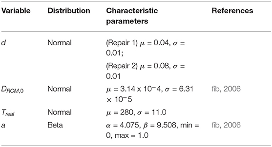
Table 2. Service life modeling parameters specific to the OFU Gimsøystraumen Bridge repair case study.

The sequence of future repairs was modeled as a Markovian chain of independent, recurring, identical deterioration and repair processes according to (15). The construction duration of any one repair activity is considered to be irrelevant when considered within the decades-long service life of the bridge.

$\begin{array}{ll}P(t_{n+1}=x|t_{n=y})=P(t_n=x|t_{n-1=y})& (15)\end{array}$

where, P is the probability that the time to the next repair will take time, t, (t_n+1) the time from most recent repair event, n, to next repair event, (n + 1), tn the time from the second most recent repair event, (n − 1), to the most recent repair event, n, (t_n−1) the time from the third most recent repair event, (n − 2), to the second most recent repair event, (n − 1), and x and y are random probabilities. Thus, the time of any future repair event (t_rj in Figure 1) is the sum of the times to repair of all previous repair events, as shown in (16).

$\begin{array}{ll}{t}_{rj}={\displaystyle \sum _{n=1}^j}(t_n(C(x=d)=C_{crit}))& (16)\end{array}$

where, t_rj is the time at which any repair, j, is performed, and t_n(C(x = d) = C_crit) the time elapsing between the performance of repair action, n, and a critical concentration of chlorides reaching the location of the reinforcing steel a distance, d, from the concrete surface. The equation shown in (16), however, can not be rearranged to create a simple output for t_rj as seen in (2) through (6), so to solve for this output, an iterative method must be implemented. For this case study the Muller Method was chosen due to its robust ability to solve for a large range of solutions regardless of the original inputted value. This is in comparison to the Newton–Raphson Method, which is more commonly used. The key difference between these two methods is that while the Newton–Raphson method uses a linear approach to solve for the x-intercept, the Muller Method uses a parabolic approach, resulting in a closer fit to the curvature of the function. More information on the Muller Method can be found in Muller (1956).

2.3.3. Environmental, Social, and Economic Impact Model of OFU Gimsøystraumen Bridge Repairs

To determine the life cycle impacts of repairs, a life cycle inventory of the repair materials, processes, and procedures was constructed. The main sources for this data were (Kompen et al., 1997), primary data from contractors, product marketing materials, personal safety and hygiene sheets (MSDS), and commercial life cycle inventory datasets. Once again, a more detailed account can be found in Lepech et al. (2014). The mechanical repair comprised five steps; (i) hydrodemolition of deteriorated concrete cover, (ii) shotcreting of replacement concrete, (iii) application of a sprayed curing membrane, (iv) sandblasting of the surface, and (v) surface treatment with an elastic mortar. For each of these steps the commercial products used, the equipment needed, and the transportation of materials to the site were cataloged. The total environmental impact is the sum of impacts from all repair steps, as shown in (17).

$\begin{array}{ll}{i}_{rj}={\displaystyle \sum _{k=1}^5}{i}_k& (17)\end{array}$

where, i_rj is the impact (social, environmental, or economic) of performing repair, j, and i_k is the impact of performing one of the five steps, k, of the mechanical repair. For demonstration purposes, global warming potential (kg CO₂-equivalents) will be used as a proxy for overall environmental impact.

The impact due to hydrodemolition, i₁, is computed as the sum total of impacts associated with water use, water for washdown purposes, waste disposal of the concrete, and impacts associated with the hydrodemolition equipment and shown in (18). The hydrodemolition equipment used includes an air compressor, a hydrodemoltion machine, and a front-end loader. Productivity rates and equipment needs were determined from RS Means Construction Cost Data (RSMeans, 2008).

$\begin{array}{ll}\begin{array}{c}{i}_1=i_{H_{2}O}{r}_{H_{2}O}d{a}_{hydro}+i_{H_{2}O}{r}_{wash}+i_{landfill}d{a}_{hydro}{\rho }_{conc}\\ +(i_{air}{r}_{air}{\gamma }_1+i_{hydro}{e}_{hydro}{\gamma }_2+i_{loader}{r}_{loader})r_{hydro}\end{array}& (18)\end{array}$

where, i₁ is the impact of hydrodemolition, i_H2O the impact of producing water in kg CO₂-eq per kg, r_H2O the rate of water use for hydrodemolition in kg per m³ of concrete removed, d the cover thickness in meters, a_hydro the area being hydrodemolished in m², r_wash the rate of water use for washdown in kg per m² of hydrodemolition, i_landfill the impact of landfilling the waste per kg, ρ_conc the density of concrete in kg/m³, i_air the impact of operating an air compressor per m² of hydrodemolition, r_air the energy consumption of an air compressor in horsepower, γ₁ is a unit conversion factor, i_hydro the impact of operating a hydrodemolition machine per m² of hydrodemolition, e_hydro the energy consumption of a hydrodemolition machine in kW, γ₂ a unit conversion factor, i_loader the impact of operating a loader per m² of hydrodemolition, r_loader the productivity of a loader in m³/hr, and r_hydro the productivity of a hydrodemolition crew in hours per m² of hydrodemolition. Distributions and parameters for these variables are provided in Table 3.

TABLE 3

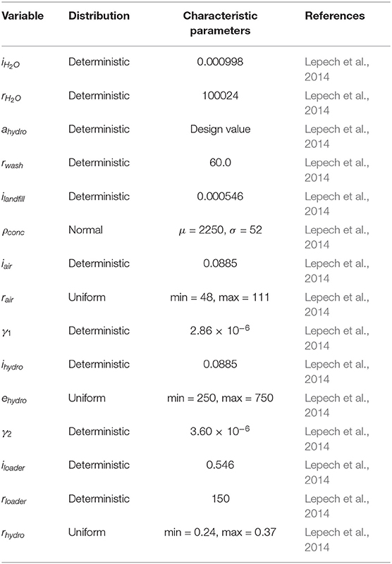
Table 3. Hydrodemolition environmental impact modeling variables, distributions, and parameters.

The impact from the shotcreting step, i₂, is computed as the sum total of impacts associated with production of the shotcrete, impacts associated with equipment on site, and impacts from transportation of the shotcrete material from the producer to the construction site, as shown in (19). The shotcrete equipment used includes an air compressor, a shotcrete rig, and a concrete pump. Productivity rates and equipment needs were determined from RS Means Construction Cost Data (RSMeans, 2008). Material proportions and species were determined from product information sheets provided by the manufacturer or environmental health and safety documentation.

$\begin{array}{ll}\begin{array}{c}{i}_2=(i_c{p}_c+i_{H_{2}O}{p}_{H_{2}O}+i_s{p}_s)d{a}_{hydro}(1+r)\\ +i_{landfill}d{a}_{hydro}(p_c+p_{H_{2}O}+p_s)r\\ +(i_{air}{r}_{air}{\gamma }_1+i_{pump}{e}_{pump}{\gamma }_2+i_{rig}{e}_{rig})r_{shot}\\ +i_{T}d{a}_{hydro}(p_c+p_{H_{2}O}+p_s)(1+r)d_{shot}{\gamma }_3\end{array}& (19)\end{array}$

where, i₂ is the impact of the shotcrete step, i_c the impact of producing cement in kg CO₂-eq per kg, p_c the proportion of cement in shotcrete in kg of cement per m³ of shotcrete, p_H2O the proportion of water in shotcrete in kg of water per m³ of shotcrete, i_s the impact of producing sand and gravel in kg CO₂-eq per kg, p_s is the proportion of sand or gravel in shotcrete in kg of sand or gravel per m³ of shotcrete, r the portion of shotcrete wasted in rebound, i_pump the impact of operating shotcrete pump per m² of hydrodemolition performed, e_pump the energy consumption of a shotcrete pump in kW, i_rig the impact of shotcrete rig truck per m² of hydrodemolition performed, e_rig the fuel consumption of a shotcrete rig truck in L of diesel fuel per hour, r_shot the productivity of a shotcrete crew in hours per m² of shotcreting repair performed, i_T the impact of truck transportation in tone-km, d_shot the distance shotcrete materials were shipped in km, and γ₃ a unit conversion factor. Distributions and characteristic parameters for these variables are provided in Table 4. Water-to-cement ratio are used to calculate p_c and p_H2O.

TABLE 4

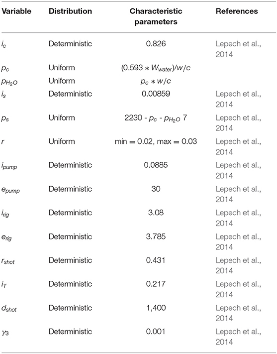
Table 4. Hydrodemolition environmental impact modeling variables, distributions, and parameters.

The impact from application of an impermeable membrane, i₃, accounts for impacts associated with production of the membrane material and impacts from transportation of materials to the construction site (20). The membrane is applied with a hand sprayer in two applications. Material proportions were determined from manufacturer product information or environmental health and safety documentation.

$\begin{array}{ll}{i}_3=(i_M{p}_M+i_N{p}_N+i_T(p_M+p_N))n_{app}{r}_{app}(1+d_{mem}{\gamma }_3)& (20)\end{array}$

where, i₃ is the impact of the membrane application, i_M the impact of producing methacrylate in kg CO₂-eq per kg, p_M the proportion of methacrylate in the membrane in kg per L of material, i_N the impact of producing naphtha in kg CO₂-eq per kg, p_N the naphtha proportion of the membrane in kg per L of material, n_app the number of applications, r_app the rate of membrane application in L per m² of repair, and d_mem the distance that materials were shipped in km. Distributions and parameters are in Table 5.

TABLE 5

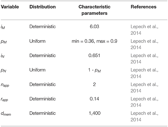
Table 5. Membrane application environmental impact modeling variables, distributions, and parameters.

The impact from sandblasting, i₄, is the sum total of impacts associated with production of the sandblasting medium, operation of an air compressor, material transportation to the construction site, and impacts from landfilling of the waste medium (21). The sand blasting medium, Star–Grit, is comprised of recycled copper slag. Material proportions were determined from manufacturer information.

$\begin{array}{ll}\begin{array}{c}{i}_4=(i_{slag}{p}_{slag}+i_s{p}_{s-slag})w_{med}+i_{air}{r}_{air}{\gamma }_1{r}_s\\ +i_{ship}{w}_{med}{d}_{sand}{\gamma }_3+i_{waste}{w}_{med}\end{array}& (21)\end{array}$

where, i₄ is the sandblasting impact, i_slag the impact of producing the slag portion of the sandblasting medium in kg CO₂-eq per kg, p_slag the slag proportion of the medium in kg of slag per kg, p_s−slag the proportion of sand in the medium in kg of sand per kg, w_med the mass of medium in kg consumed per m² of sandblasting, r_s the crew productivity in hours per m², i_ship the impact of ship transportation in tone-km, and d_sand the shipping distance in km. Distributions and parameters are in Table 6.

TABLE 6

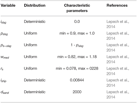
Table 6. Sandblasting environmental impact modeling variables, distributions, and parameters.

The impact from surface treatment of the repair, i₅, is computed as the sum total of impacts associated with production of the surface treatment materials and impacts from transportation of the surface treatment materials to the construction site, as shown in (22). No mechanical equipment is used in the application of the surface treatment. Material proportions and species were determined from product information sheets provided by the manufacturer or environmental health and safety documentation.

$\begin{array}{ll}{i}_5=i_c{p}_{c-surf}+i_s{p}_{s-surf}+i_L{p}_{L-surf}+i_T{w}_{surf}{d}_{surf}{\gamma }_3& (22)\end{array}$

where, i₅ is the impact of the surface treatment, p_c−surf the proportion of cement used in the surface treatment mortar in kg per m² of surface treatment, p_s−surf the proportion of sand used in the surface treatment mortar in kg per m², i_L the impact of producing the latex portion of the surface treatment mortar in kg CO₂-eq per kg of latex, p_L−surf the proportion of latex used in the surface treatment mortar in kg per m², w_surf the mass of surface treatment mortar in kg consumed per m², and d_surf the distance that materials were shipped in km. Distributions and characteristic parameters are provided in Table 7.

TABLE 7

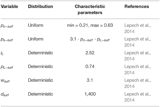
Table 7. Surface treatment environmental impact modeling variables, distributions, and parameters.

3. Results

Using SIPmath in Microsoft Excel, modeling of cumulative impact envelopes, shown schematically in Figure 1, was done using a total of ten interdependent workbooks. The model is interactive, such that the user can change the repair thickness, d, the mean and standard deviation of the ambient temperature, T_real, the water-to-cement ratio, which ultimately affects the chloride migration coefficient, D_RCM,0, mean and standard deviation, the area of concrete being evaluated, as well as the mean, standard deviation, minimum, and maximum critical chloride concentration, C_crit. Additionally, the spreadsheet allows for modifications of the percentiles of the data defining the envelope, allowing for the envelope to be modified based on user preferences and requirements. To allow for comparison, two independent plots are created next to each other in the main dashboard of the spreadsheet. Each of these plots are seeded identically but have separate alterable inputs, allowing for comparable probabilistic variables between designs.

For illustration, the cumulative impact was predicted for an 80-year analysis period for each of the repairs considered (0.04 and 0.08 m) as shown in Figures 2A,B, respectively. A 1m² area of concrete was used as a functional unit, and all other values were considered constant across the two designs. A water to cement ration of 0.45 was used, resulting in the desired diffusion coefficient.

FIGURE 2

Figure 2. Cumulative global warming potential envelopes (kg CO₂-eq/m²) for (A) 0.04 m, (B) 0.08 m repair, and (C) 0.04 m repair + 2°C timelines. For all three, the 20th, 50th, and 80th percentiles are plotted, as is one example timeline (Trial 100).

As seen in Figure 2, increasing cover thickness from 0.04 to 0.08 m effectively reduced total carbon emissions over an 80-year analysis period. Also, by the end of 80 years there is enough difference in the CO₂-eq emissions of the 0.04 and 0.08 m timelines to give confidence that the 0.08 m repair is the more sustainable choice. This can then be confirmed by calculating probability of failure.

The 0.04 m design results in a greater impact than the 0.08 m design as discussed previously, so for probability of failure calculations, the 0.04 and 0.08 m designs are the sustainable target value and design impact respectively. A reduction factor is also applied to the target to allow the user to set their design goals to a fraction of the original design based on ecological carrying capacity. For this case study a 10% reduction target is applied to the target. This means that the user is trying to reduce the impacts of the initial design by at least 10%. Probability of failure is then calculated in the spreadsheet using a simulation based approach. This simulation contained 10,000 trials. The results of this at 5 year intervals can be seen in Figure 3. At the beginning of the lifespan, the probability of failure is 1. This is expected since neither of the designs have any impact yet. However, as the bridge ages the probability of failure decreases due to the longer times in between repairs of the 0.08 m design.

FIGURE 3

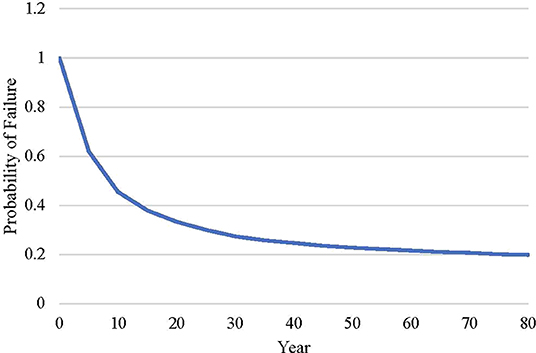
Figure 3. Simulation based probability of failure at 5 year intervals for 0.04 and 0.08 m case.

Due to the uncertainties when using simulation based probability of failure calculations, these calculations are validated using traditional probabilistic methods in MATLAB, shown in (14). Table 8 shows a comparison of these two results at 5 year intervals as well as the percent error in the simulation based calculation. The values for percent error range between 0 and 3.43%. A graphical comparison of the two results is shown in Figure 4. It can be concluded from this figure that the results are comparable, validating the calculation methodology used in the spreadsheet.

TABLE 8

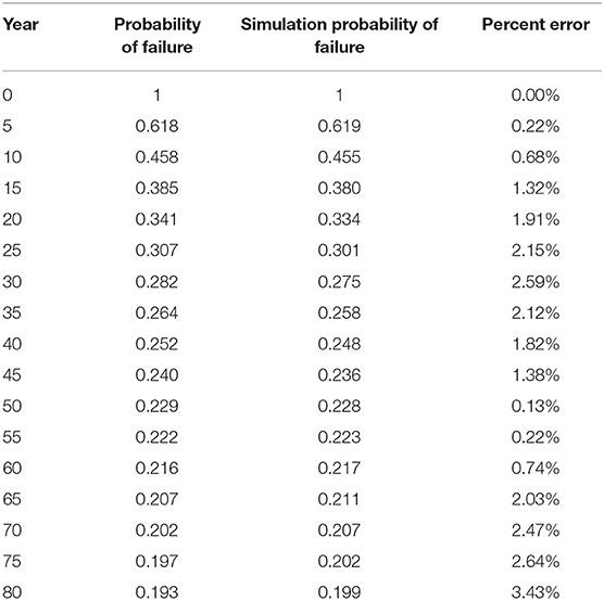
Table 8. Comparison and percent error of probability of failure calculation methods for 0.04 and 0.08 m case.

FIGURE 4

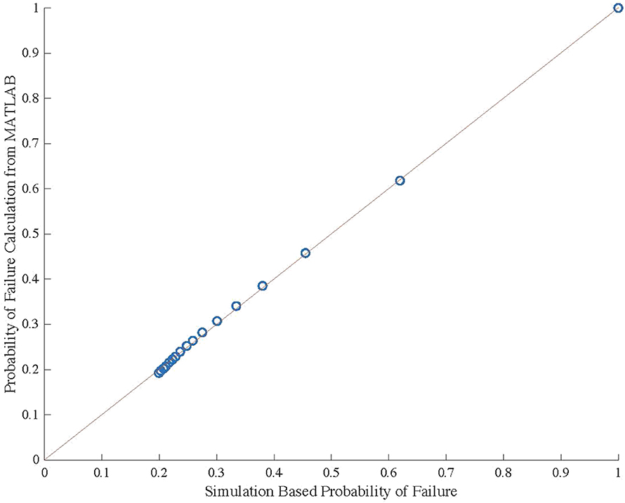
Figure 4. Graphical comparison of probability of failure calculation methods for 0.04 and 0.08 m case.

Taking the model further, the effect of climate change can be explored. Figure 2C shows the cumulative envelope for a 0.04 m repair timeline under a temperature rise of 2°C (IPCC, 2013). While slight, there is a noticeable increase in the cumulative global warming potential for timelines exposed to higher temperatures. Given that these results are only for one square meter of repairs over an 80-year analysis period, the results become more concerning when considering the myriad concrete repairs performed annually worldwide. Moreover, the vicious cycle of carbon emissions leading to temperature rise, leading to faster deterioration of concrete infrastructure, leading to more repairs, leading to increased carbon emissions becomes clearer to decision-makers. This clarity is motivation for the development of easy-to-use probabilistic modeling and design tools using SIPmath modeling.

Additionally, the effects on overall impact can be observed due to variation in mix design. A higher ratio of cement within a concrete mix leads to a lower diffusion coefficient, lengthening the time between repairs. However, the relationship between water-to-cement ratio and diffusion coefficient is non-linear, so the effects on impact are not as intuitive. Figure 5 shows a probability of failure comparison between two 0.04 m designs with a water-to-cement ratio of 0.40 and 0.45. An increase in cement does result in a decreasing probability of failure as the bridge ages, but these results are not as significant as increasing cover depth. This model not only allows for users to see how a change in the design will effect the impact but also allows for different alterations to be compared to evaluate effectiveness.

FIGURE 5

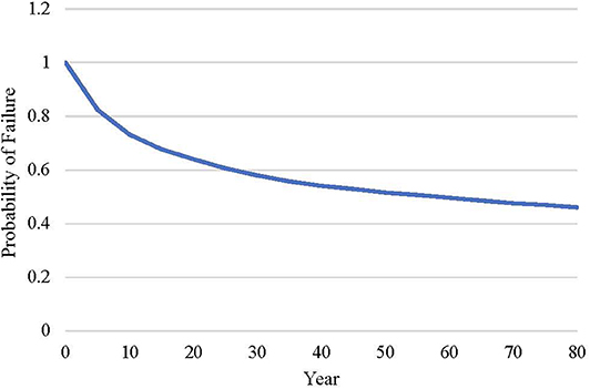
Figure 5. Simulation based probability of failure at 5 year intervals for water-to-cement ratios of 0.45 and 0.40.

Though the results of these comparisons may seem predictable without the assistance of a model, this spreadsheet allows for more complex comparisons, where several values are altered. Additionally, it allows for analysis of the complex, non-linear relationship between variables. This complex relationship can be observed in the probability of failure plot shown in Figure 6, comparing a 0.04 m design with a water-to-cement ratio of 0.45 to a 0.08 m design with a water-to-cement ratio of 0.40. The change in water-to-cement ratio does not significantly impact the overall probability of failure as much as one would expect. This is due to the non-linear relationship between water-to-cement ratio and diffusion coefficient. From this analysis it can be concluded that a change in water to cement ratio is not the best decision when attempting to reduce overall impact.

FIGURE 6

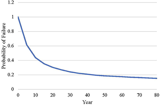
Figure 6. Simulation based probability of failure at 5 year intervals for a 0.04 m design with a water-to-cement ratio of 0.45 and a 0.08 m design with a water-to-cement ratio of 0.40.

Finally, the highly non-linear relationship between variables can be analyzed using a sensitively analysis. This spreadsheet allows for quick iterations of calculations, making the process of conducting a sensitivity analysis simple and efficient. Table 9 shows a simple example of how this can be executed. This table compares how a single alteration of a variable affects the probability of failure, showing which variables have the largest impact on reducing probability of failure. The values used in the table are chosen because they are reasonable values for the given variable and ensure a more sustainable design. It can be observed from this sensitivity analysis that depth has the largest impact on probability of failure, while standard deviation of temperature and standard deviation of critical chloride concentrations have a minimal effect on probability of failure.

TABLE 9

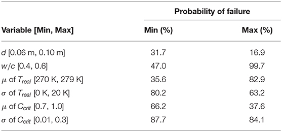
Table 9. Sensitivity analysis.

4. Discussion

This paper presented a probabilistic framework for the design of civil infrastructure that achieves targeted improvements in quantitative sustainability indicators. The framework consists of two types of models; (i) probabilistic service life prediction models, and (ii) probabilistic life cycle assessment (LCA) models. Specifically, this paper introduced a new mathematical approach, SIPmath, to simplify sustainability-focused design and potentially accelerate its adoption by infrastructure designers. The model's implementation in Excel as well as its lack of direct application of complex probabilistic tools makes it easy to use for practicing structural engineers. Additionally, the flexibility of the inputs in the spreadsheet allow for quick iterations of calculations, making the tool practical for use in industry. A reinforced concrete bridge repair in Norway was presented as a case study to demonstrate SIPmath implementation.

Ultimately, the case study showed that SIPmath tools can provide designers and engineers an engaging tool for sustainability-focused probabilistic design of reinforced concrete infrastructure. The analysis showed that a 0.08 m concrete repair was preferable to a 0.04 m concrete repair over the 80-year analysis period of the OFU Gimsøystraumen Bridge. This was also confirmed using probability of failure calculations. It was also verified that simulation based probability of failure calculation is a accurate method for assessing probability of failure. Additionally, the effect of a 2°C increase in annual average temperature associated with global climate change had a noticeable effect on the cumulative carbon emission profile of the case study bridge. Finally, the non-linear relationship between input variables was demonstrated to show how the model can be used for more complex design decisions.

There are limitations in this study both in the service life model and the impact model. The service life model implemented in this case study uses Fickian diffusion. This is a simple method to approach diffusion of chloride and does not capture all aspects of the complex nature of this process. However, many different limit state models can be implemented using this framework with SIPmath. These models can be ultimate limit state models or serviceability limit state models and vary in complexity, so a more complex model can be implement to correct for this limitation. The limitations of the impact model are due to the probabilistic and deterministic data used for calculations. Uncertainty in this data is due to uncertainties in completeness, temporal correlation, geographic correlation, further technological correlation, and sample size.

Data Availability Statement

The datasets generated for this study are available on request to the corresponding author.

Author Contributions

MZ wrote the article and created the overall concept. SS provided SIPmath expertise. ML, MG, HS, and AM provided deterioration modeling expertise.

Funding

The authors thank the support of the Thomas V. Jones faculty scholarship at Stanford. This research is partly funded by the US NSF (Award #1453881). Any opinions, findings, and conclusions or recommendations expressed in this material are those of the authors and do not necessarily reflect the views of the NSF.

Conflict of Interest

SS was employed by company Probability Management Inc.

The remaining authors declare that the research was conducted in the absence of any commercial or financial relationships that could be construed as a potential conflict of interest.

References

Abramowitz, M., and Stegun, I. (1983). Handbook of Mathematical Functions with Formulas, Graphs, and Mathematical Tables. Washington, DC: Dover Publications.

Google Scholar

Bakshi, B., Ziv, G., and Lepech, M. (2015). Techno-ecological synergy: a framework for sustainable engineering. Environ. Sci. Technol. 49, 1752–1760. doi: 10.1021/es5041442

PubMed Abstract | CrossRef Full Text | Google Scholar

Blankvoll, B. (1998). OFU Gimsøystraumen bru, Hovedresultater og Oversikt over Sluttdokumentasjon: Publication 89. Vegdirektoratet, Veglaboratoriet, Oslo.

Comello, S., Lepech, M., and Schwegler, B. (2012). Project level assessment of environmental impact: An ecosystem services approach to sustainable management and development. ASCE J. Manage. Eng. 27, 5–12. doi: 10.1061/(ASCE)ME.1943-5479.0000093

CrossRef Full Text | Google Scholar

Ehrenfeld, J. (2007). Would industrial ecology exist without sustainability in the background? J. Indus. Ecol. 11, 73–84. doi: 10.1162/jiec.2007.1177

CrossRef Full Text | Google Scholar

fib (2006). Model Code for Service Life-Bulletin 34. FIB, Lausanne.

fib (2010). 2010 Model Code - Bulletin 55, 56. FIB, Lausanne.

IPCC (2013). Climate Change 2013, United Nations Intergovernmental Panel on Climate Change (IPCC) 5th Assessment Report. United Nations Intergovernmental Panel on Climate Change, New York, NY.

ISO (2006). ISO 14040: LCA–Principles and Framework. International Organization for Standards, Geneva.

Kompen, R., Blankvoll, A., Berg, T., Noremark, E., Austnes, P., and Grefstad, K. (1997). OFU Gimsøystraumen bru: Prøvereparasjon og Produktutvikling: Publication 84. Vegdirektoratet, Veglaboratoriet, Oslo.

Lepech, M. (2018). The future design of sustainable infrastructure. Natl. Acad. Eng. Bridge 48, 13–21.

Google Scholar

Lepech, M., Geiker, M., Stang, H., and Michel, A. (2014). Sustainable Rehabilitation of Civil and Building Structures. Department of Civil Engineering (BYG), Technical University of Denmark (DTU), Lyngby.

Lepech, M., Stang, H., and Geiker, M. (2013). Probabilistic design and management of environmentally sustainable repair and rehabilitation of reinforced concrete structures. Cements Concrete Composites 47, 19–31. doi: 10.1016/j.cemconcomp.2013.10.009

CrossRef Full Text | Google Scholar

Muller, D. (1956). A method for solving algebraic equations using an automatic computer. Am. Math. Soc. 10, 208–215. doi: 10.2307/2001916

CrossRef Full Text | Google Scholar

RSMeans (2008). Heavy Construction Cost. Reed Construction Data, Kingston, MA. doi: 10.1680/clh.2008.2008.9.177

PubMed Abstract | CrossRef Full Text | Google Scholar

Russel-Smith, S., and Lepech, M. (2015). Cradle-to-gate sustainable target value design: integrating life cycle assessment and construction management for buildings. J. Clean. Product. 100, 107–115. doi: 10.1016/j.jclepro.2015.03.044

CrossRef Full Text | Google Scholar

Russel-Smith, S., Lepech, M., Fruchter, R., and Meyer, Y. (2015). Sustainable target value design: integrating life cycle assessment and target value design to improve building energy and environmental performance. J. Clean. Product. 88, 43–51. doi: 10.1016/j.jclepro.2014.03.025

CrossRef Full Text | Google Scholar

Savage, S., and Thibault, J. (2015). “Towards a simulation network or the medium is the Monte Carlo,” in The 2015 Winter Simulation Conference, eds L. Yilmaz, I. C. Moon, W. Chan, T. Roeder, C. Macal, and M. Rosetti (Huntington Beach, CA: Institute of Electrical and Electronics Engineers, Inc), 4126–41333.

Google Scholar

Scrivener, K., John, V., and Gartner, E. (2018). Eco-efficient cements: potential economically viable solutions for a low-co₂ cement-based materials industry. Cement Concrete Res. 114, 2–26. doi: 10.1016/j.cemconres.2018.03.015

CrossRef Full Text | Google Scholar

Vu, K., and Stewart, M. (2000). Structural reliability of concrete bridges including improved chloride-induced corrosion models. Struct. Saf. 22, 313–333. doi: 10.1016/S0167-4730(00)00018-7

CrossRef Full Text | Google Scholar