Optimal Static Load Compensation With Fault Tolerance in Nonlinear Adaptive Structures Under Input and State Constraints

1. Introduction

Lightweight structures are a reality for many mass-sensitive applications, such as large civil engineering structures. In the most cases, the designs of passive structures present a minimum in terms of required mass under given safety limitations and user comfort constraints. However, it is possible to stay within these limits while further reducing the total embodied mass significantly by introducing active structures, which is referred to as ultra-lightweight design. Through their various actuators, these structures can react and adapt to external loads and disturbances – both static and dynamic. This is done in order to minimize element stresses and at the same time maximize lifetime expectancy. Even lighter designs are possible compared to passive lightweight structures. In light of the expected construction activities within the next 20–30 years (OECD, 2015), and in line with the ongoing population growth as estimated by the UN (Department of Economic and Social Affairs), the world-wide trend of urbanization will further increase in pace, as projected by the UN (Department of Economic and Social Affairs). Ultra-lightweight designs can thus help save millions of tons of concrete and steel and significantly reduce waste production and CO₂-emissions of the construction industry.

One of the first research results on adaptive engineering structures was published by Yao (1972). Just a few years later, Kirsch and Moses (1977) proposed an active control strategy for a single beam subject to several single loads, but their findings strongly supported the idea of increased loading capacity or reduced cross section dimensions through the use of mechanisms for active compensation. Since then, the field has evolved, but it has nevertheless remained a rather small community, as it requires an interdisciplinary approach bringing together civil and control engineering. Recent overviews about structural control, including several passive, semi-active, and active approaches, have been provided by Korkmaz (2011), Housner et al. (1997), and Spencer and Nagarajaiah (2003). Most of the literature focuses on dynamic problems, i.e., active vibration control for damping oscillations. For example, Gawronski (2004) and Preumont (1997) use model-based approaches for the control design. Literature on the compensation of static loads by active structures is problem specific. A broad overview of current developments in structural control in Europe can be found in Basu et al. (2014), who give several case studies. Case studies that focus on energy and cost assessment of adaptive structures are presented in Senatore et al. (2018a). Insight into an approach for influence matrices is given in Reksowardojo and Senatore (2020), where the integrated force method is compared with a force method based on singular value decomposition.

From a practical point of view, the literature on active vibration control is manifold. Different aspects have to be taken into account such as input constraints due to actuator size, force limitations, as well as state constraints due to the need for keeping inhabitants comfortable. The authors of Johnson and Erkus (2002) present a semi-active optimal control approach for a structural control problem, for which the semi-active damping device is modeled by input constraints. Active vibration control with active mass dampers of seismically excited multi-story building is done by Materazzi and Ubertini (2012). To incorporate input constraints in the proposed linear quadratic regulator (LQR), the problem is augmented, introduction of a virtual unsaturated input and a nonlinear map between augmented state and virtual input. For this system, the state-dependent Riccati equation is solved. A backstepping approach to control seismic motion of structures was proposed by Amini and Ghaderi (2013). This approach guarantees the limitation of control forces while at the same time improving closed loop system performance. The algorithm is illustrated on a three-story building.

There are tensegrity structures that can be associated, to a certain extent, with the structure considered in this contribution. Adam and Smith (2008) designed a multi-objective shape controller that selects a pareto optimum based on the applied load and is additionally improved by reinforcement learning. This approach is validated on an experimental setup of a tensegrity structure covering 15 m². Fest et al. (2003) specifically included geometric nonlinearities in their modeling approach of an active tensegrity structure and applied a stochastic search algorithm to determine the control inputs. In comparison to pure tensegrity structures, we consider a structure that is stiffened by tension-only diagonal bracings that are barely prestressed and therefore buckle under compression, which has been studied for tensegrities by Alart et al. (2007). Nevertheless, our structure also incorporates beam elements that bear tension, compression, and even bending and torsion, many strategies that work for tensegrities cannot thus be simply applied here.

Sobek and Teuffel (2001) proposed a method for static control of structures by minimizing element forces or displacements in a simple optimization without consideration of input or state constraints. In this paper, adaptivity is considered during the design process already, which eventually leads to a more sustainable structure. More recently, Neuhäuser et al. (2013) and Neuhäuser (2014) showed static load compensation for a double-curved shell in order to minimize peak stresses in the structure. Experimental validation is also given. Senatore et al. (2019) introduced a methodology for optimal design of adaptive structures while minimizing the whole-life energy consumption by regarding embodied energy and operational energy needed during operation to perform any necessary adaption. Their approach has been experimentally validated with an adaptive truss prototype, see Senatore et al. (2018b).

Static shape control is performed for two- and three-dimensional bodies such as beams, shells, or plates. For example, Irschik and Ziegler (2001) and Irschik et al. (2000) conducted static shape control by performing an eigenstrain analysis to determine the control forces that can compensate the quasi-static deflection of the body through external forces. Piezoelectric actuators are used to manipulate the body's stress distribution. The analysis and design are based on distributed parameters theory and thus cannot simply be transferred to our discretized finite element (FE) model. The authors of this publication have, however, also studied this aspect and Wagner et al. (2019b) presented an example for static load compensation on a beam modeled by a distributed parameters system.

The application of adaptive structures and static control is a wide field in aerospace engineering, regarding satellites with positioning of measurement equipment or wings of airplanes to adapt for wind flows. Sener et al. (1994) focused on statically indeterminate structures and investigated static control and actuator placement. As noted by Pellegrino (1990), it is important to separate between statically determinate and indeterminate structures because the number of independent force states in a structure is—as mentioned by Wagner et al. (2018)—coupled to the static indeterminacy. Sener et al. (1994) aimed at enlarging the stress in a structure. Therefore, the authors mainly work with statically indeterminate and prestressed structures. Several examples are given for illustration. For large space structures, Matunaga and Onoda (1995) presented a control law for optimal shape control with respect to modeling errors for elements and actuator forces. They further performed actuator placement by means of an integer optimization problem, where they specifically included several actuator failure cases in the optimization to increase the fault tolerance of the entire structure. This is highly relevant for space applications due to the limited maintenance options. A different approach of actuation was taken by Haftka and Adelman (1985), who used nonuniform heating to control deformation of adaptive structures governed by continuous or discrete equations. Saggere and Kota (1999) regarded an airplane wing as a smart structure, where principles of mechanics and kinematics are coupled with an optimization program to achieve smooth shape changes using a single actuator.

Previous works of our group have considered the problem of actuator placement for structures under static loads (e.g., Wagner et al., 2018; Böhm et al., 2019) and under dynamic loads (e.g., Heidingsfeld et al., 2017), as well as dynamic modeling and nonlinear damping control of structures with tension-only elements (e.g., Wagner et al., 2019a) and enhanced with decentralized control (e.g., Wagner et al., 2020). Böhm et al. (2020) focus on modeling and successful integration of different types of actuation principles into existing FE-models of passive structures. A relation is derived between actuators included in series and in parallel. First results on fault-tolerant control for active shape control of a double-curved shell were given by Heidingsfeld et al. (2015), where faults in actuators were treated as additional constraints in the optimization to derive the input signals. Recent results on fault detection and diagnosis were published by Gienger et al. (2020), and convolutional neural networks were used on the various input and sensor signals to detect and isolate actuator and sensor faults.

This article contributes to the modeling and control of adaptive structures with tension-only elements where some of these are equipped with serially integrated actuators, which renders the equations more complex and naturally leads to input constraints. More specifically, the main contribution of this article is the derivation and validation of a load compensation method based on numerical minimization of deformations due to static loads that particularly includes input and state constraints. Validation of the proposed algorithms is performed on an experimental setup with 25 actuators evaluating element forces and position measurements of the structure. Proving the real world applicability of the strategy, a 1:18 scale model is used. Finally, the potential to rerun the optimization with a reduced set of actuators is demonstrated, which enhances the fault-tolerance of adaptive structures.

The article is organized as follows: Section 2 introduces the nonlinear modeling including tension-only elements for a given structure. Additionally, inputs and outputs are modeled. In section 3, the optimal control strategy is introduced to conduct static load compensation and the treatment of faults in actuators. Experimental and numerical results are illustrated and discussed in section 4. Finally, a conclusion and outlook are given.

2. System Modeling

This section derives the nonlinear, stationary model equations of an adaptive high-rise structure. These serve as the basis for the following optimal load compensation. For the sake of completion, first, a linear system model is introduced, on top of which nonlinear structural elements are incorporated.

2.1. Linear Equations of Motion

Assuming stationary conditions, the physical states of a stationary civil engineering structure are computed by means of the finite element method (FEM). The vector q ∈ ℝⁿ denotes the nodal degrees of freedom (DOF) in translational and rotational directions and is also called state of the system. In particular these modeling equations are represented by

$\begin{array}{ll}Kq=f(u)\text{ with }f(u)=Fu+Ez,y=Cq,& (1)\end{array}$

where K ∈ ℝ^n×n is the stiffness matrix, and f(u) comprises actuator forces u ∈ ℝ^m and disturbances z ∈ ℝ^k. The input matrix F ∈ ℝ^n×m describes the actuator topology for m active elements. The disturbance matrix E ∈ ℝ^n×k represents stationary external loads, for example, snow loads or static wind loads. Each column of this matrix, each contains the distribution of external forces over all degrees of freedom for a single load case. The overall external load is given as a linear combination of these individual disturbance vectors with the respective amplitudes defined in z. The system's output y ∈ ℝ^l captures measurement values and can be calculated by means of the output matrix C ∈ ℝ^l×n and the systems state.

2.2. Nonlinear Equations of Motion

In practice, structures may not be accurately represented by the linear system model (1). Common nonlinear structural elements are bracings, which serve the purpose of stiffening an entire structure. For example, a cable or flat steel both introduce nonlinearities because these elements can only bear tension forces and therefore slacken under compression. This effect leads to a state dependent stiffness matrix K(q). In the case of a compressed nonlinear bracing element, the corresponding entry k_i of the stiffness matrix does not contribute to the structure's stiffness:

$\begin{array}{ll}{k}_i(q)=\{\begin{array}{cc}{k}_i,& \Delta l_i(q)\ge 0\\ 0,& \Delta l_i(q)<0\end{array}i=1,...,n_t.& (2)\end{array}$

The total amount tension-only elements is denoted by n_t. The switching condition between tension and compression depends on the length difference of an element

$\begin{array}{ll}\Delta l_i(q)=\sqrt{\Delta {\tilde{q}}_i^{⊺}\Delta {\tilde{q}}_i}-\sqrt{\Delta q_{i,0}^{⊺}\Delta q_{i,0}}.& (3)\end{array}$

The last term represents the initial length of an element with Δq_i,0 = q_i,1,0 − q_i,2,0, where q_i,1,0 and q_i,2,0 are the initial absolute positions given in a global coordinate system of the nodes to which element i is attached to. The first term yields the current length of the element i, where the individual positions of the associated nodes have to be represented in a global coordinate system.

$\begin{array}{ll}\Delta {\tilde{q}}_i={\tilde{q}}_{i,1}-{\tilde{q}}_{i,2}& (4)\end{array}$

In the above equation, the absolute reference position of the nodes ${\tilde{q}}_{i,1}$ and ${\tilde{q}}_{i,2}$ are equal to ${\tilde{q}}_{i,1}=q_{i,1,0}+q_{i,1}$ and ${\tilde{q}}_{i,2}$, respectively, where the relative displacements of the attachment nodes are a subset of the DOF vector, i. e., q_i,1 ⊂ q and q_i,2 ⊂ q. If changes in the element's stiffness k_i(q) in function (2) apply, the structure's stiffness matrix K(q) has to be reassembled, leading to a state-dependent formulation of (1):

$\begin{array}{ll}K(q)=f(u),y=h(q,u).& (5)\end{array}$

Consequently, the system's output is stated as a general nonlinear function depending on the state and the input. Nevertheless, in most cases the output is given by a linear function of the form h(q, u) = Cq. Nonlinearities of the kind (2) can be considered in structural analysis using any common FE-software. The system formulation (5), however, is required for the purpose of model-based control design (ref. section 3) within a tool as Matlab or Python. A system formulation for dynamic analysis of this type of nonlinearities was derived by Wagner et al. (2019a, 2020).

2.3. Actuation Principles and Input Modeling

In this study, two actuation principles are introduced, and their implication on the adaptive structure is analyzed. The first principle, shown in Figure 1A, considers a force parallel actuator, which is essentially an additional (active) link that can influence the truss structure. Changing the length of this actuator leads to the same length change in the parallel element due to the fact that both elements are attached to identical nodes. However, the forces in the actuator and the parallel (passive) element are potentially very different. These depend on the cross sectional areas of the active and passive element and are determined as a function of the actuator force, while the structure is required to reach an equilibrium state.

FIGURE 1

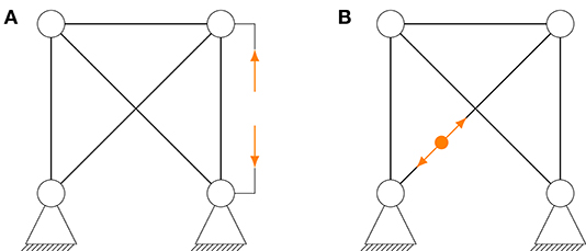
Figure 1. Two actuation principles for adaptive structures (A) parallel force and (B) serial force.

Due to the parallel elements, this actuation principle might seem to lead to an overdesigned configuration. However, it enables actuation of highly loaded elements and has benefits in terms of safety and fault tolerance. Such elements are mainly included in the load path to compensate a structure's dead load. Consequently, since the actuator is not required to completely bear the static dead load, it can be used for damping purposes or to generate small scale manipulations and structural deformations. Moreover, the actual passive element can be designed for much smaller dynamic loads because dynamic load components are transferred to the actuator. Together, both can be designed such that they are not necessarily heavier than a single passive column.

The second principle is the serial actuation depicted in Figure 1B. In this configuration, the actuator is included in the load path of an element so that the force in the element is directly set by and equal to the actuator's force. If the structure is not in an equilibrium, the element will extend or shorten its length until the element force is equal to the actuator's force. In duality with the parallel actuation principle, the displacement of the passive part of the element and the actuator add up to the total change in length between the two nodes (Böhm et al., 2020). The element and actuator force are equal. As it was concluded in Wagner et al. (2018), a serial actuation principle for bracing elements is preferred, which stiffen a structure. Regardless of the chosen principle, all actuator forces will be limited in practice according to the design. Since typical bracing elements can only be stressed in tension, as explained in section 2.2, serial actuators are not capable of exerting compression forces in such elements.

A mechanical limit in the actuators needs to be installed for safety reasons to prevent undesired large deformations of the structure. If the actuator hits its upper limit stop and the force within this active element is higher than the upper force limit of the actuator, an impact on the structure is not possible¹. Furthermore, actuation is lost, in the case of a fully contracted actuator, if the active element is compressed. Therefore, all inputs generated by actuators, which are connected in series, are state dependent. This is modeled by means of a state-dependent input matrix B_s(q). The basic equations for including serial actuation into a given model are given by Böhm et al. (2020), and the input function can be separated as follows:

$\begin{array}{ll}f(u_{\text{s}},u_{\text{p}})=B_{\text{s}}(q)u_{\text{s}}+B_{\text{p}}{u}_{\text{p}}+Ez.& (6)\end{array}$

Consider a number of serial actuators, m_s, and a number of parallel actuators, m_p. The causality between the actuation and the DOF is described by the respective input matrix $B_{\text{s}}(q)\in {ℝ}^{n\times m_{\text{s}}}$ and $B_{\text{p}}\in {ℝ}^{n\times m_{\text{p}}}$. The input forces of both types of active elements are $u_{\text{s}}\in {ℝ}^{m_{\text{s}}}$ and $u_{\text{p}}\in {ℝ}^{m_{\text{p}}}$. The external loads, which cannot be affected, are captured in the last term Ez. Given a parallel setup in which each individual actuation is represented by $b_i^{⊺}{u}_{\text{p},i}$, the actuation force of a corresponding serial configuration (leading to the same equilibrium state of the structure) is calculated by

$\begin{array}{ll}{u}_{\text{s},i}=u_{\text{p},i}-k_i{b}_i^{⊺}q.& (7)\end{array}$

if the element's stiffness k_i is known. The question of where the actuators are placed within the structure is addressed in earlier contributions. For active vibration control under dynamic loads, actuators can be placed according to Heidingsfeld et al. (2017) by means of the Gramian controllability matrix with integrated spillover reduction. For static load compensation, a placement strategy was proposed in Wagner et al. (2018) in which a cost function is derived based on certain load assumptions. Appropriate assumptions can be formulated in order to achieve optimality under a wide range of loading events. However, an adaptive structure's set of actuators needs to provide high performance for a variety of loads. The final choice of the actuator set for any kind of adaptive structure must be a combination of these results obtained for the various loads—static and dynamic—eventually considering symmetry and economic aspects as well.

2.4. Output Modeling

Different outputs may be considered in adaptive structures. This section focuses on two relevant types of outputs, which are used in optimization and for evaluation. These are the nodal displacements and the element forces.

2.4.1. Displacement

In civil engineering, rather strong restrictions apply to the displacements of high-rise buildings due to comfort reasons. A common rule is the horizontal displacement of the tip of a building is restricted within a range that does not exceed 0.2–0.5 % of the building's height. In order to test this restriction, we need to define the nodal displacement output:

$\begin{array}{ll}{y}_{\text{disp}}=C_{\text{disp}}q.& (8)\end{array}$

Only the translational DOFs are considered via the output matrix C_disp, as there are typically no (strong) restrictions on the rotational DOFs.

2.4.2. Element Forces

As discussed in section 2.2, tension-only elements, common link elements, and different actuator types are complex to consider in terms of element forces in output modeling. Therefore, the N_e element forces are captured in $y_{\text{force}}(q)\in {ℝ}^{N_{\text{e}}}$, which comprises four parts. Firstly, element forces $y_{\text{force},\text{s}}(q)\in {ℝ}^{N_{\text{s}}}$ of tension-only elements with serial actuation are considered. Secondly, element forces $y_{\text{force},\text{p}}\in {ℝ}^{N_{\text{p}}}$ of all (link or beam) elements with parallel actuation are included. Thirdly, element forces $y_{\text{force},\text{sp}}(q)\in {ℝ}^{N_{\text{sp}}}$ of tension-only elements without actuation are captured. Finally, the remaining element forces, $y_{\text{force},\text{r}}\in {ℝ}^{N_{\text{r}}}$:

$\begin{array}{ll}{y}_{\text{force}}(q)={\left[\begin{array}{cccc}{y}_{\text{force},\text{s}}^{⊺}(q),& y_{\text{force},\text{p}}^{⊺},& y_{\text{force},\text{sp}}^{⊺}(q),& y_{\text{force},\text{r}}^{⊺}\end{array}\right]}^{⊺}.& (9)\end{array}$

All element forces are normal forces and are calculated in dependence of the actuation type and the element type. For tension-only elements actuated in series, where the actuator is operating within its stroke limits, the element force is equal to the actuator force. If the actuator hits the upper stroke limit, the force exerted on the element by the structure's displacement can be higher than the actuator force. This force is calculated in the same way as for passive elements using an adapted stiffness constant of the combined element. If the actuator is fully contracted and the element is slackend, no force is transmitted over the element. In summary, the force output of each individual element i is expressed:

$\begin{array}{ll}{y}_{\text{force},\text{s},\text{i}}(q)=\{\begin{array}{cc}{C}_{\text{force},\text{s},\text{i}}q,\hfill & \Delta l_i(q)\ge 0\hfill \\ u_{\text{s},\text{i}},\hfill & \Delta l_{i,\text{min}}<\Delta l_i(q)<0\hfill \\ 0,\hfill & \Delta l_i(q)<\Delta l_{i,\text{min}}\hfill \end{array},\hfill & (10)\end{array}$

where Δl_i,min is the lower actuator stroke limit and 0 its upper stroke limit. For the elements actuated in parallel

$\begin{array}{ll}{y}_{\text{force},\text{p}}=C_{\text{force},\text{p}}q+D{u}_{\text{p}}& (11)\end{array}$

holds. The first term represents the force transferred through the passive part, while the second term represents the actuator force. With the notation adopted, the actuator force is positive when the actuator acts against its compression. Since compression forces are typically defined with a negative sign, the matrix D is defined as D = −I. Any passive tension-only element only transfers forces if it is under tension, while the element forces are zero under compression:

$\begin{array}{ll}{y}_{\text{force},\text{sp},\text{i}}(q)=\{\begin{array}{cc}{C}_{\text{force},\text{sp},\text{i}}q,\hfill & \Delta l_i(q)\ge 0\hfill \\ 0,\hfill & \Delta l_i(q)<0.\hfill \end{array}\hfill & (12)\end{array}$

The remaining elements are common tension and compression (link or beam) elements with

$\begin{array}{ll}{y}_{\text{force},\text{r}}=C_{\text{force},\text{r}}q.& (13)\end{array}$

Equations (9)–(13) are summarized in the nonlinear output function h(q) to obtain

$\begin{array}{ll}{y}_{\text{force}}(q)=h(q)q.& (14)\end{array}$

All output matrices $C_{\text{force},(·)}\in {ℝ}^{(·)\times n}$ contain the matched stiffness and geometric information, i.e., the stiffness of the individual elements and to which nodes the respective elements are attached to.

3. Control

In this section, a model-based control strategy for optimal static load compensation for nonlinear adaptive structures under state and input constraints is introduced. While for linear control, a variety of analytic control schemes are available, static compensation for the nonlinear model is best tackled by an optimization-based algorithm, as proposed in section 3.2. The required optimization metric is explained in section 3.1. Finally, a simple adaption scheme for reconfiguration of the compensation control is given for the case of actuator faults in section 3.3.

3.1. Optimization Metric

For this contribution, we chose to minimize the nodal displacements of the structure. Therefore, the cost function consists of the quadratic sum of all nodal displacements and is given by

$\begin{array}{ll}J(q)=y_{\text{disp}}^{⊺}{y}_{\text{disp}}=q^{⊺}{C}_{\text{disp}}^{⊺}{C}_{\text{disp}}q.& (15)\end{array}$

Another possible optimization metrics is the homogenization of element forces over all elements, which was used as a metric for actuator placement by Böhm et al. (2019). For this, the stress in an element is calculated and set in relation to its yield strength. This utilization quantity is homogenized over all elements by penalizing deviations from the mean utilization value in the cost function.

3.2. Static Load Compensation

Static load compensation is realized by minimizing the cost function introduced above under given constraints regarding the structure's displacement as well as state and input constraints. One common requirement for high-rise buildings is the limitation of the structure's displacement to 0.2–0.5 % of a building's height. In the following, the approach for optimal static load compensation including all constraints is given using the nonlinear model together with serial and parallel actuated elements.

3.2.1. Optimization

The optimization problem to determine the optimal parallel and serial inputs for a given static load by minimizing the displacement of the structure under constraints with the cost function taken from (15) described by

$\begin{array}{ll}\left\{u_s^{*},u_p^{*},q^{*}\right\}=\text{arg}{\displaystyle \underset{u_s,u_p,q}{\text{ min}}}J(q)& (16)\end{array}$

$\begin{array}{l}\text{s}.\text{t}.K(q)=B_{\text{s}}(q)u_{\text{s}}+B_{\text{p}}{u}_{\text{p}}+Ez\\ u_{\text{s},\text{min}}\le u_{\text{s}}\le 0\\ u_{\text{p},\text{min}}\le u_{\text{p}}\le u_{\text{p},\text{max}}.& (17)\end{array}$

The optimization variables in (16) are the parallel and serial inputs u_p and u_s. Note, that the state-dependent stiffness matrix K(q) can become singular as soon as too many tension-only elements are actually under compression. Thus, invertibility of K(q) cannot be guaranteed and therefore, the state vector q cannot be calculated by inversion of K(q). We have thus reformulated the optimization with the steady state equation as an equality constraint rendering the state q an additional optimization variable. This avoids inversion of K(q) but leads to a higher number of optimization variable as a consequence. The input constraints can be explained as follows: the serial input signals can only transmit tension forces and therefore must have a negative value. The largest tension force is given by |u_s,min|. The parallel actuators can generate tension and compression forces and stay within the limits of u_p,min and u_p,max. Since only static loads are considered, constraints of time-dependent values, e. g., acceleration or velocities, can be neglected. In the present paper, we assume a known static load, while, in practice, static load estimation is a complex task that is beyond the scope of this contribution.

The optimization is started with an initial condition, corresponding to the state of the passive structure under the given load. The parallel and serial input u_p and u_s are concatenated to u = [u_p, u_s]. The input u is calculated analytically for the system linearized around q = 0:

$\begin{array}{ll}u=-{(C{K}^{-1}(0)B)}^{+}(C{K}^{-1}(0)Ez),& (18)\end{array}$

where B = [B_p, B_s]. Note that the initial conditions might not satisfy state and input constraints.

3.3. Fault Tolerance and Reconfiguration

In large and complex systems with many actuators and sensors, robustness with respect to faults is an important property. In this contribution, we focus on actuator faults and assume the detection of faults is available (e.g., as proposed by Gienger et al., 2020). Through the potential of the large number of actuators, it is possible to reconfigure control to provide high control performance despite faults. After detecting an actuator fault, an obvious approach is the recalculation of control signals with a reduced number of actuators. This is acceptable, if the calculation time of the optimization stays below the time constants of the system dynamics. In this article, we consider only quasi-stationary loads, which is an important load case for civil engineering structures, and the optimization program is solved in way shorter time. Furthermore, as initial condition, the preceding solution without actuator faults is used as the reconfigured solution is expected to be close. So, the optimization problem is solved for a changed actuator configuration using (16) and (17). In an additional step, it would be possible to include constraints induced through faulty actuators, e.g., an actuator cannot move further and remains at an arbitrary but fixed length.

4. Numerical and Experimental Results

In this section, the numerical and experimental results are depicted and discussed. At first, the investigated structure is explained, and, subsequently, the results for optimal static load compensation and reconfiguration are given.

4.1. System Description

4.1.1. General Setup

To illustrate the results of optimal static load compensation, a scale model of an adaptive high-rise structure is used. The full size adaptive high-rise structure will be constructed on the site of the University of Stuttgart, rendered in Figure 2A. The structure will be a twelve story building with 36 m height covering a square base with side length of 4.7 m, detailed information is given by Weidner et al. (2018). The scale model investigated in this contribution is 18 times smaller, leading to a height of 2 m and a square ground base of 0.26 × 0.26 m (see Figure 2B). It is subdivided into five modules, where one module comprises two stories. The module and story numbering start at the bottom with index 1. The full-size building comprises four modules with three stories each.

FIGURE 2

Figure 2. (A) Rendering of the full-size adaptive high-rise structure (left) and the access tower (right) (© ILEK), (B) picture of the 1:18 scale model, and (C) sketch of the scale model with actuator and sensor equipment and load mounting.

Four vertical elements, eight diagonal bracings, and one plate are mounted per module, where the element numbering is given in Figure 3. Instead of plates, the full-size building will feature horizontal bracings where modules meet. Additionally, the plates are assumed to be very rigid and are therefore excluded in the calculation of element forces. Sensors are installed in terms of strain gauges in almost each vertical and diagonal element. Furthermore, an optical measurement system is installed to measure some of the nodal displacements (ref. Figure 2). Strain gauges are mounted onto the base material of the elements and the small measurement signals are amplified. The optical sensors measure the nodal displacement of one side of the building (Figure 2C). The green light emitters are detected with a camera system (Ximea MC023MG-SY) on two sides of the building to get spatial information on the structure's displacement with submillimeter resolution. The full-scale building will be equipped with the same sensor setup, adapted to the larger scale. Additionally, sensors for wind, rain, and solar radiation will be installed to estimate external loads. A construction to excite the scale model statically is shown in the scheme. A weight of m_load = 4 kg, and, by this, about 40 N are applied to the top of the scale model horizontally in x-direction. In modeling, the load is divided upon the upper two nodes on the right side. A shaker table is installed below the scale model, exciting the structure in x- and y-direction for investigating the dynamic behavior. As providing this kind of excitation is too complex for the full-scale building, a subset of the integrated actuators will be used instead to simulate excitation. Every module incorporates a microcontroller, which communicates sensor and actuator signals to the central control unit. The optical measurement system directly communicates its measurements via ethernet to the central control unit. All microcontrollers are connected to the central control hardware (dSpace MicroLabBox DS1202) via CAN-bus. All algorithms are implemented using Matlab/Simulink and executed using the dSpace MicroLabBox along with the software dSpace ControlDesk. A summary of geometry and material parameters are given in Table 1.

FIGURE 3

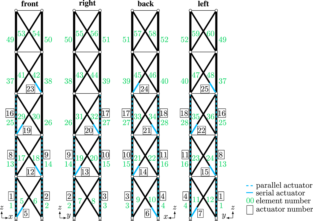
Figure 3. Actuated elements with numbering of the actuators.

TABLE 1

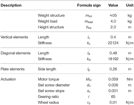
Table 1. Geometry and material parameters of the scale model.

4.1.2. Actuators

Parallel actuators are integrated in 11 vertical elements, as depicted in Figure 2C. The integration of active components in a column is shown at the top of Figure 4. A brushless DC motor (Faulhaber 2264W024BP4 3692—operated by a motor controller Faulhaber MC5010) is mounted at the bottom of each active column. The motor is coupled to a ball screw to transform rotation to a linear motion. The nut is clamped between two springs, which directly determine the stiffness of a column. The lower end of the lower spring and the upper end of the upper spring are connected via the housing and are referred to as grounding. Therefore, the springs are mounted in a parallel setup. The corresponding actuation principle is sketched in Figure 1. The structure also incorporates 14 active diagonal bracings, see Figure 2C for the locations. Diagonal elements are realized by steel cables, which are wound over a roll that is connected to a worm gear. A brushless DC motor is mounted on the other end of the worm gear. The top module is a passive part of the structure, i.e., no actuators are installed in the top module. Actuator and element numbers are given in Figure 3. The full-scale building includes a similar actuator set; however, due to the absence of the fifth module the following changes occur. The third module does not include vertical actuators, and the forth module contains no actuators at all, leading to only 24 active elements. These actuators will be realized as hydraulic cylinders. The full-scale model will be the main experimental setup to validate and evaluate all developed control algorithms, including static compensation as well as active vibration control, observer strategies and fault detection.

FIGURE 4

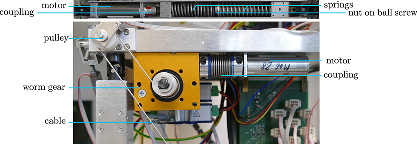
Figure 4. Construction of parallel actuation in the columns (Top, rotated by 90°) and serial actuation for diagonal elements (Bottom).

The values for inequality constraints are calculated based on Table 1 such that u_s,min = −111 N, u_p,min = −296 N and u_p,max = 296 N. The actuator forces in the setup for serial and parallel actuation cannot be measured directly. The motors are velocity controlled by the motor controllers. To apply the desired serial actuator force, an underlying PI-controller was designed for each motor, which uses the strain gauge measurement to control the current element force. Due to the strain gauge installation, the serial element force is measured, from which the corresponding parallel element force can be calculated using (7). The feedback gains for the parallel and serial actuators are designed separately. The error is defined as the difference between desired and measured value. The P- and the I-gains multiplied with the errors for the parallel actuators are k_P = −1 and k_I = −10 and for the serial actuators k_P = −20 and k_I = −80.

4.2. Static Load Compensation

The optimization problem (16), (17) was solved by means of an interior-point algorithm as proposed by Wächter and Biegler (2006)². On a development PC (Intel Core i@2.7GHz), computation time of the optimization for the given parameters and initial condition is approximately 3 s, which is sufficient for static adaption. Displacement results are presented for both the simulated and measured structures and an illustration of the measured element forces is provided.

4.2.1. Displacements

Figure 5 shows the qualitative results of the static load compensation of the experimental setup with the reference state in Figure 5A. The structure stands upright without actuation; however, serial actuation needs to be turned on and set to an initial value to apply a minimal prestress as a valid starting point from which to apply compensating input signals. The worm gear is self-locking, and the force is preserved without motor interference thereafter. Figure 5B displays the structure under the load without actuation. In Figure 5C, the displacements induced by the load are compensated by using the motors and the optimized input signals.

FIGURE 5

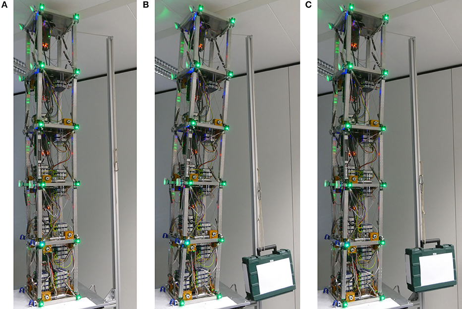
Figure 5. Photographs of the experimental setup of the scale model. (A) Upright state as reference, (B) applied load without compensation, and (C) compensation of the displacement caused by the load.

Position measurements are compared to the simulation results in Figure 6. These measurements are obtained from the cameras of the optical measurement system, and an offset is applied based on the reference state measurements. Figure 6A shows the measurement points in xz-plane for the reference, loaded, and compensated states. The effect of the load is almost completely compensated for, as seen by the reduction in displacement from 11.5 to 0.3 cm at the top. Deviations form the reference state are mainly visible in the middle of the structure, and they are reduced from 4.6 to 1.3 cm at the end of the second module. In general, perfect compensation cannot be reached for all loads. The deviation in the middle is due to the locations of the serial actuation. The actuated diagonal elements go from the bottom right to the top left in the second module and therefore they cannot counteract the induced displacement. Thus, only the actuation in the columns is available, which is not sufficient for the required compensation. Regarding actuator placement, various static loads were investigated justifying the present actuator configuration (Wagner et al., 2018). While, for this specific load, another actuator configuration would have been beneficial, the model's actuator setup is chosen as a compromise between the optimal placement for several different load cases. Figure 6B displays measurement and simulation results for the scale model under load. According to the simulation, the expected displacement is larger than the measured displacement. The simulation model assumes a homogenous structure with constant parameters for passive and active elements. However, the upper modules do contain mostly passive elements. Especially the diagonals in these modules are prestressed to avoid slack even in the initial straight upright position. Therefore, the upper modules seem more rigid and are not as much displaced in the experiments compared to the simulation results. Figure 6C shows the compensation of the displacement of the structure under load for the real setup and simulation. The optimization results are applied to the motors and almost completely compensate for the initial displacement. The deviation from the reference state is not visible for the simulation. This discrepancy can be partly explained by asymmetric actuator placement in the model. Furthermore, a model is only a limited approximation of the real world behavior and leaves out effects, e.g., nonlinear effects, such as hysteresis and stick-slip in the actuated columns and diagonal bracings. In general, the results of the position measurements show sufficient accuracy and performance and a very good static load compensation.

FIGURE 6

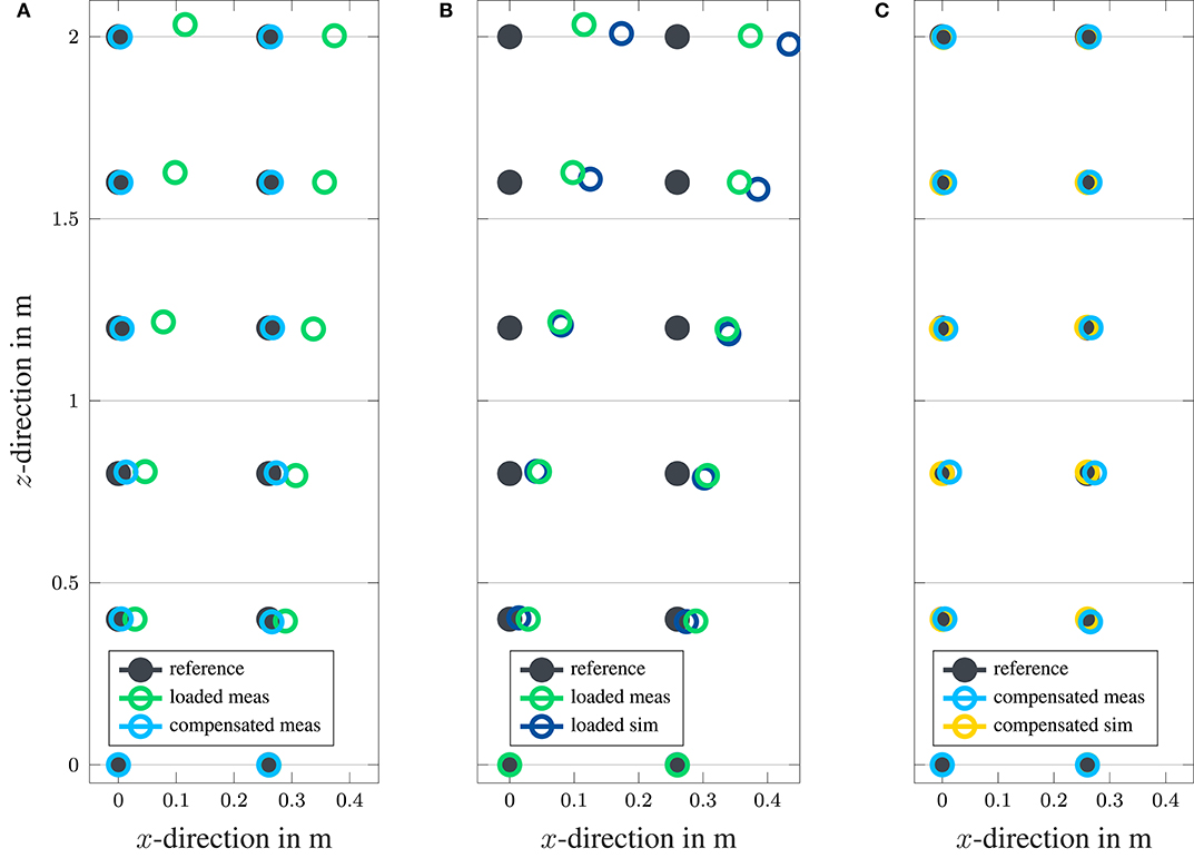
Figure 6. Comparison of position data for measured (meas) and simulated (sim) models with the reference state (gray). (A) Measured positions for the loaded state (green) and compensation of the displacement (light blue). (B) Loaded structure measurement (green) and simulation (dark blue). (C) Compensated measurement (light blue) and simulation (yellow). The data is summarized in Table A1 (top) in the Appendix.

4.2.2. Actuator Forces

For an illustration of the actuator forces, the parallel and serial inputs are named according to the actuator number in Figure 3 and summarized to one sorted input u. Figure 7 shows the actuator forces determined by the optimization algorithm. Serial forces are depicted directly, while parallel actuation forces are calculated with (7) to obtain the element force. As expected, under the given load, the actuators in columns 1, 4, 8, 11, 16, and 19 need to apply tension forces, while column actuators 2, 3, 9, 10, and 17 apply compression forces. All diagonal actuators show, as required, only non-positive forces (i.e., tension). All input constraints due to the actuator force limits are met. The asymmetry in the actuator forces is due to the asymmetric actuator locations. In module three, only three columns are actuated and in module one and four, three diagonals are actuated.

FIGURE 7

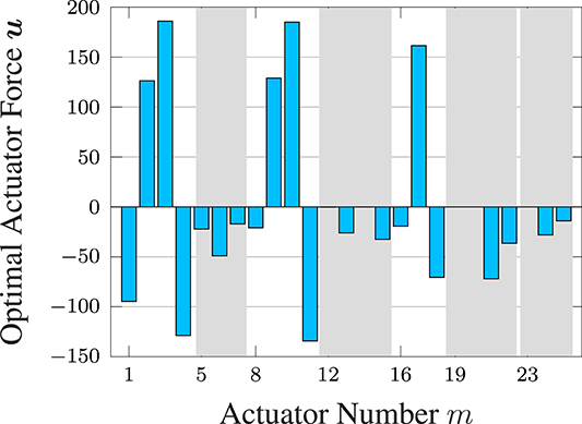
Figure 7. Calculated optimal actuator forces for each actuator. Serial actuators are marked by a gray background.

For the forces in the columns, the zero-offset value cannot be determined in the mounted state. Therefore, the reference value of the upright state is set as the zero-offset value. For active and passive tension-only elements, the zero-offset value was determined in advance by slackening the cables.

To evaluate the actuation forces, the desired and the measured element forces are depicted over the actuator number in Figure 8. Actuator numbers are given in Figure 3. Serial actuators are highlighted by a gray background. In Figure 8A the results for the structure under load are shown, where actuation for compensation is turned off. However, the serial actuated elements are controlled such that the element force from the prestress in the reference state is maintained. Otherwise, if these elements were fixed, they would be stretched and exhibit high element forces, induced by the load. That is the reason why desired element forces for the serial actuated elements are shown in this plot. Desired forces are matched by actual measured forces to a sufficient extent. Some of these actuated tension-only elements are slack, which is shown by values close to/below zero (see actuator 14, and 15). Values below zero are possible since the zero-offset value can only be determined within a few Newtons. Actuators 13, 20, 23, and 24 do not reach their desired forces due to the limited motor torque. Due to the loading, the structure stretches these elements. Therefore, higher forces cannot be reached. Actuator 6 is set to a lower tension force in the element, but does not achieve it. Due to safety reasons, a mechanical stroke limit stop was installed for the serial actuators to avoid complete release of several tension-only elements, which would lead to a collapse of the structure. In the full-scale structure, mechanical stroke limits are installed as well to meet legal requirements. Figure 8B illustrates the forces of the actuated elements in the case of active load compensation. In columns 1, 2, 3, 4, and 8, the desired forces are reached with high accuracy. For columns 11, 16, and 17, small deviations from the desired values are visible; however, an acceptable accuracy is still achieved. The vertical elements 9, 10, and 18 show large discrepancies from the desired value. Possible reasons for this are mainly constraints in the motor torques, especially with respect to the reference state. Such constraints are considered in the optimization, but due to the unknown zero-offset value, the reference state may have had larger than anticipated initial loads.

FIGURE 8

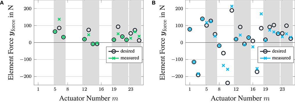
Figure 8. Measured element forces of the actuated elements (crosses) and the desired element forces (circles). Serial actuators are marked by a gray background. Element forces of the structure under load (A) without compensation and (B) with compensation. The data is summarized in Table A2 in the Appendix.

4.2.3. Element Forces

To illustrate the effects of the load and the compensation on the whole structure, element forces are displayed by means of colored plots. Tension forces are depicted in red and compression forces in blue. The darker the color, the higher the element's force. The plates are indicated by horizontal lines and are not equipped with sensors. Diagonal tension-only elements in black are slack. Two diagonal elements in the fifth module and one in the second module had faulty strain gauge sensors (see Figure 2C) and are also marked in black. Diagonal elements show absolute forces, while columns are shown in reference to the initial upright state because absolute force could not be determined in the mounted state. Active elements are marked by a circle, keeping in mind that the element force of diagonal elements is controlled solely by the motors. Active columns are only controlled in the compensated state.

When the load is applied, as shown in Figure 9, columns on the left side experience high tension forces, while columns on the right are mostly subject to compression forces. Small tension forces appear in element 15; however, in comparison to the reference state, compressive loading has reduced these forces. Element 26 is the only passive column in the third module and shows slightly different behavior than the active columns. Furthermore, this element is shorter by a few millimeters due to construction. The upper two modules seem to be stiffer, as already visible in Figure 6A, and bending of these modules is lower than expected from the simulation. This is caused by the construction of the passive columns. In Figure 10, the element forces of the structure under active load compensation are depicted. In the columns on the left, tension forces are reduced due to a more upright position compared to the uncompensated state. On the right side, compression forces are reduced for the same reason; however, in element 14, the force is reduced only marginally. Owing to the limitations of the motor torque, this compression force remains at a high level. Moreover, the column above, number 26, is the only passive column in module three. The fifth module is almost unchanged due to the absence of actuators. Regarding the columns, the fourth module also shows a similar force distribution with and without compensation.

FIGURE 9

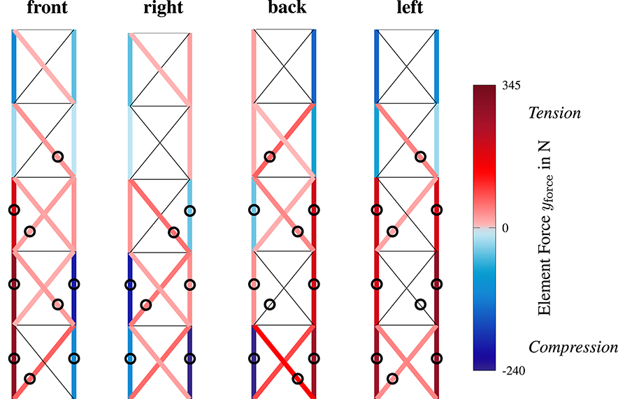
Figure 9. Measured element forces for the structure under load and without compensation, as in Figure 5B. Tension is indicated in red and compression in blue. Actuated elements are marked with a circle. The title indicates the viewing direction.

FIGURE 10

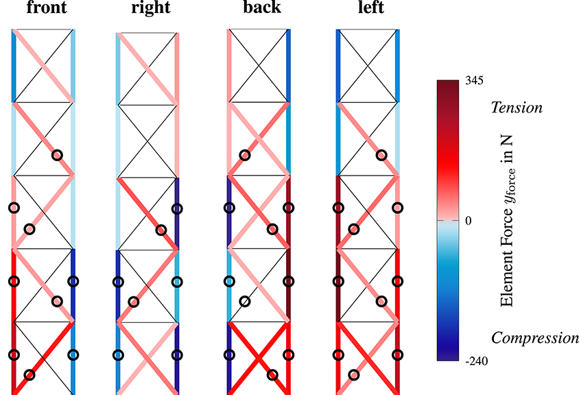
Figure 10. Measured element forces for the structure under load and with active compensation, as in Figure 5C. Elements without a color are unmeasured or slack. Tension is indicated in red and compression in blue. Actuated elements are marked with a circle. The title indicates the viewing direction.

When considering the diagonal elements, the prestress of each individual element has a large impact on the structure's behavior. Diagonal 5, which is also actuated, exhibits a higher force when the compensation is enabled as is calculated through the optimization. Visually speaking, this diagonal pulls back the structure to an upright state, which appears intuitively right. Element 10 should show a similar behavior; however, this element is at its stroke limit in the uncompensated case, which can be seen in Figure 8A, since the desired force is not reached in that case. In general, actuators in diagonal bracings on the right can only marginally counteract the load-induced nodal displacements. Nevertheless, in the nonlinear model, a slight influence is present and actuation forces are obtained from the optimization (see Figure 8). In the second module, the active diagonals cannot counteract the displacement through the load due to their tension-only capability. Further tensioning of these active elements would enlarge the displacement, therefore, the optimized actuator forces are zero for elements 18 and 21, which corresponds to actuator number 12 and 14 (see Figure 7). Element 22, which contains actuator number 15, exhibits zero force in the uncompensated load case due to the low prestress in the reference state. During compensation, the optimal actuator force is reached, and the element is under tension. The third module shows similar behavior as the first module because the actuator configuration is similar. Element 30 is slack in the uncompensated load case but is under tension in the compensated state.

In general, evaluation of this multiple input multiple output (MIMO) system is quite challenging because small changes in a single actuator influence many elements. Furthermore, the sheer amount of output data complicates evaluation and bookkeeping of the system and its measurements. However, the experiment provides a proof of concept and showed that using the proposed method of optimal static load compensation for structures with tension-only elements and feasible input and state constraints, a significant reduction of nodal displacements could be achieved in the experimental testing. Force distribution in active and passive elements is reasonable and the structural behavior that is to be expected for the actual high-rise demonstrator is also well-illustrated.

4.3. Fault Tolerance and Reconfiguration

It is assumed that faults are detected in the column actuators 3 and 4 and are therefore no longer functional. The optimization problem as defined by (16), (17) is adapted and rerun with updated parameters compensating for the missing actuators. The displacement results are shown in Figure 11. The displacements of the structure using the optimal actuation signals under the assumption of faulty actuators are shown against the compensation assuming fully functioning actuators. On a development PC (Intel Core i@2.7GHz), computation time of the optimization is approximately 2 s. The lower value is mainly due to using the preceding solution as the initial condition, obtained for the faultless case. After reconfiguration and calculation of actuator signals for the current actuator set, the performance of load compensation is comparable to the performance with all actuators. For a small number of faulty actuators, it is possible to still achieve a very good load compensation due to the large overall amount of actuators. With an increasing number of faulty actuators, it will become difficult to maintain functionality. However, when faults occur, prompt actuator maintenance will be implemented such that safety of inhabitants and surrounding structures and persons is guaranteed. Figure 12 depicts actuator signals of the adapted configuration in comparison to the optimal result with all actuators. Actuation signals for actuator 3 and 4 are missing. Actuation force of other actuators rise, especially in the first module where the faulty actuators are located. Diagonal tension-only actuator efforts that contribute to pulling the structure back into an upright position, e.g., actuators 5, 8, 12–15, 19, and 20, are increased to compensate for the missing actuators. Other actuation forces are reduced such that the structure is not deformed in an undesired way. Forces from diagonal actuators 6 and 7 are reduced and are directly interacting with the faulty actuators. Tension from these actuators, adds forces in the negative x- and z-directions of the element with faulty actuator 3. This would align the structure more upright; however, it would also pull down the z-coordinate. To balance this, the optimization returns no input signal for actuator 7. Reconfiguration under a small number of faulty actuators is an important capability because performance losses can be avoided and functionality and safety can be maintained until maintenance.

FIGURE 11

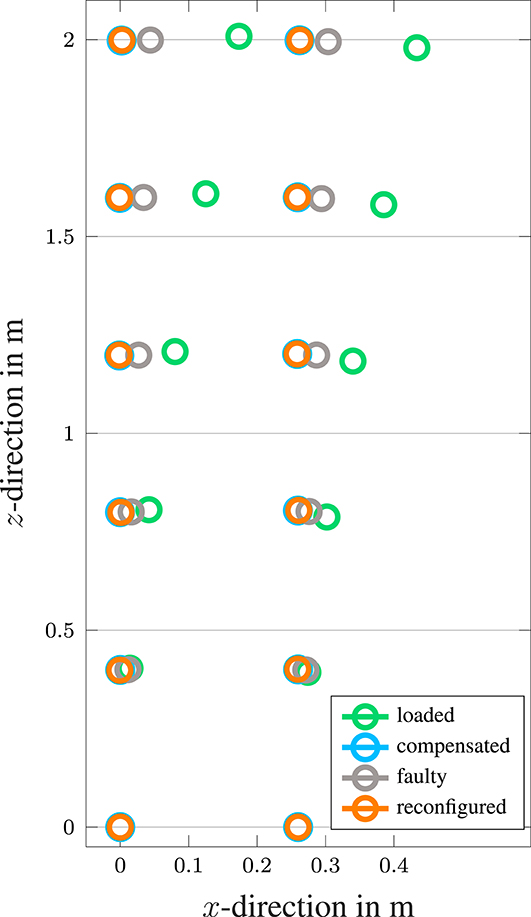
Figure 11. Position data for a reduced actuator set due to actuator faults: the optimal input including all actuators (gray), the reconfigured optimal input for the reduced actuator set (orange), passive structure under load (green), and compensated state where all actuators are functional (light blue). The reduced actuator set does not include column actuator 3 and 4 due to actuator faults. The data is summarized in Table A1 (bottom) in the Appendix.

FIGURE 12

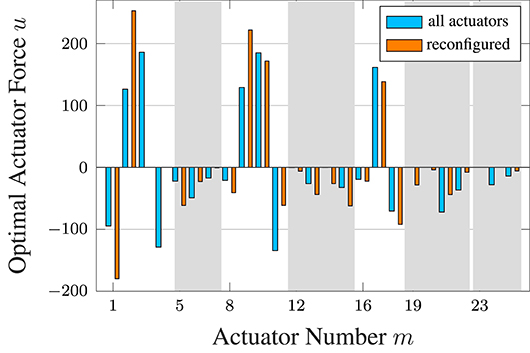
Figure 12. Optimal actuator forces over the actuator number for all actuators available (blue) and for the reduced actuator set (orange). Serial actuators have a gray background.

5. Conclusion and Outlook

In this work, we have presented a modeling approach for adaptive structures comprising of tension-only elements with serial and parallel actuation. Based on this model, an optimization-based approach for optimal static load compensation was introduced and demonstrated by means of an experimental setup. A drastic reduction of the structure's displacements was achieved such that safe operation of an adaptive building can be guaranteed, establishing a comfortable environment for inhabitants. Input constraints due to actuator saturation and state constraints due to comfort limits of a structure were both considered in the optimization formulization and were not violated by the results. The measured compensation results were all well within a limit of h_tot/100. Results from the simulation and experiment aligned, however, there were errors as it seems the overall stiffness is higher than in simulation since the simulated displacements due to the applied load are clearly higher than the measured displacements. This holds especially for the upper two modules. Despite containing only three actuators, the results obtained from the optimization using the simulation model still provided a very good compensation. The performance of the algorithm degrades when faulty actuators are present. However, when these faults can be detected and the control signals are reconfigured accordingly, it is possible to restore the original performance, provided there is a sufficient number of remaining actuators. This kind of fault tolerance is a necessary property in control of civil engineering structures.

In this context, eigenstrain analysis can be an applicable tool. However, one has to investigate the feasibility with respect to the present nonlinearities. A proper starting point could be the method presented in Reksowardojo et al. (2020), which considered eigenstrain analysis geometric nonlinearities due to large shape changes. Furthermore, measurements regarding the energy consumption of the static control strategy on the scale model are planned. For the next step, we will integrate the load estimation to achieve applicability in a full size adaptive structure. We plan to apply this strategy to the full size adaptive structure and provide the respective experimental validation. Static load compensation and active vibration control need to be incorporated in a single control scheme, such that the effect of various loads can be compensated.

Data Availability Statement

All data used in and recorded for this study are available from the authors upon request.

Author Contributions

MB, JW, and AG contributed to the presented methodology. CS, JW, AG, and MB conducted the implementations. JW, AG, and MB wrote sections of the manuscript. PA was responsible for the experimental hardware where measurements were conducted. OS and CT provided approval for publication. All authors intensively and critically discussed the content, contributed to manuscript revision, read, and approved the submitted version.

Funding

The authors gratefully acknowledge the generous funding of this work by the German Research Foundation (DFG—Deutsche Forschungsgemeinschaft) as part of the Collaborative Research Centre 1244 (SFB) Adaptive Skins and Structures for the Built Environment of Tomorrow, B04, B03, A06, Z01.

Conflict of Interest

The authors declare that the research was conducted in the absence of any commercial or financial relationships that could be construed as a potential conflict of interest.

Footnotes

1. ^However, this would be a strong indicator for a poorly chosen actuator design.

2. ^We used here the implementation of the OPTI Toolbox, a free MATLAB Toolbox for Optimization by Inverse Problems Ltd. from 2014. More information can be found online at: https://www.inverseproblem.co.nz/OPTI/index.php/Main/HomePage.

References

Adam, B., and Smith, I. F. (2008). Active tensegrity: a control framework for an adaptive civil-engineering structure. Comput. Struct. 86, 2215–2223. doi: 10.1016/j.compstruc.2008.05.006

CrossRef Full Text | Google Scholar

Alart, P., Dureisseix, D., Laniel, R., and Pagano, S. (2007). “Wires and cables in some discrete structures of civil engineering,” in 6th Eurosim Congress on Modelling and Simulation (Ljubljana).

Google Scholar

Amini, F., and Ghaderi, P. (2013). Seismic motion control of structures: a developed adaptive backstepping approach. Comput. Struct. 114, 18–25. doi: 10.1016/j.compstruc.2012.09.011

CrossRef Full Text | Google Scholar

Basu, B., Bursi, O. S., Casciati, F., Casciati, S., Del Grosso, A. E., Domaneschi, M., et al. (2014). A European association for the control of structures joint perspective. Recent studies in civil structural control across Europe. Struct. Control Health Monit. 21, 1414–1436. doi: 10.1002/stc.1652

CrossRef Full Text | Google Scholar

Böhm, M., Steffen, S., Gade, J., Geiger, F., Sobek, W., Bischoff, M., et al. (2020). “Input modeling for active structural elements–extending the established Fe-workflow for modeling of adaptive structures,” in International Conference on Advanced Intelligent Mechatronics (Vancouver, BC).

Google Scholar

Böhm, M., Wagner, J., Steffen, S., Sobek, W., and Sawodny, O. (2019). “Homogenizability of element utilization in adaptive structures,” in IEEE 15th International Conference on Automation Science and Engineering (CASE) (Boston), 1263–1268.

Google Scholar

Fest, E., Shea, K., Domer, B., and Smith, I. F. C. (2003). Adjustable tensegrity structures. J. Struct. Eng. 129, 515–526. doi: 10.1061/(ASCE)0733-9445(2003)129:4(515)

CrossRef Full Text | Google Scholar

Gawronski, W. (2004). Advanced Structural Dynamics and Active Control of Structures. New York, NY: Springer Science & Business Media. doi: 10.1007/978-0-387-72133-0

CrossRef Full Text | Google Scholar

Gienger, A., Ostertag, A., Böhm, M., Bertsche, B., Sawodny, O., and Tarín, C. (2020). Data-based distributed fault diagnosis for adaptive structures using convolutional neural networks. Unmanned Syst. 8, 221–228. doi: 10.1142/S2301385020500156

CrossRef Full Text | Google Scholar

Haftka, R. T., and Adelman, H. M. (1985). An analytical investigation of shape control of large space structures by applied temperatures. AIAA J. 23, 450–457. doi: 10.2514/3.8934

CrossRef Full Text | Google Scholar

Heidingsfeld, M., Arnold, E., Tarín, C., and Sawodny, O. (2015). “Actuator fault-tolerant control of the stuttgart smartshell,” in 2015 IEEE Conference on Control Applications (Syndney), 996–1001. doi: 10.1109/CCA.2015.7320742

CrossRef Full Text | Google Scholar

Heidingsfeld, M., Rapp, P., Böhm, M., and Sawodny, O. (2017). “Gramian-based actuator placement with spillover reduction for active damping of adaptive structures,” in Proc. of the IEEE/ASME International Conference on Advanced Intelligent Mechatronics (Munich), 904–909. doi: 10.1109/AIM.2017.8014133

CrossRef Full Text | Google Scholar

Housner, G., Bergman, L., Caughey, T., Chassiakos, A., Claus, R., Masri, S., et al. (1997). Structural control: past, present, and future. J. Eng. Mech. 123, 897–971. doi: 10.1061/(ASCE)0733-9399(1997)123:9(897)

CrossRef Full Text | Google Scholar

Irschik, H., Krommer, M., and Pichler, U. (2000). Shaping distributed piezoelectric self-sensing layers for static shape control of smart structures. J. Struct. Control 7, 173–189. doi: 10.1002/stc.4300070204

CrossRef Full Text | Google Scholar

Irschik, H., and Ziegler, F. (2001). Eigenstrain without stress and static shape control of structures. AIAA J. 39, 1985–1990. doi: 10.2514/2.1189

CrossRef Full Text | Google Scholar

Johnson, E., and Erkus, B. (2002). “Structural control with dissipative damping devices,” in Proc. of the American Control Conference, Vol. 3 (Anchorage, AK: IEEE), 2463–2468. doi: 10.1109/ACC.2002.1024013

CrossRef Full Text | Google Scholar

Kirsch, U., and Moses, F. (1977). Optimization of structures with control forces and displacements. Eng. Optim. 3, 37–44. doi: 10.1080/03052157708902375

CrossRef Full Text | Google Scholar

Korkmaz, S. (2011). A review of active structural control: challenges for engineering informatics. Comput. Struct. 89, 2113–2132. doi: 10.1016/j.compstruc.2011.07.010

CrossRef Full Text | Google Scholar

Materazzi, A. L., and Ubertini, F. (2012). Robust structural control with system constraints. Struct. Control Health Monit. 19, 472–490. doi: 10.1002/stc.447

CrossRef Full Text | Google Scholar

Matunaga, S., and Onoda, J. (1995). Actuator placement with failure consideration for static shape control of truss structures. AIAA J. 33, 1161–1163. doi: 10.2514/3.12540

CrossRef Full Text | Google Scholar

Neuhäuser, S. (2014). Untersuchungen zur homogenisierung von spannungsfeldern bei adaptiven schalentragwerken mittels auflagerverschiebung (Dissertation). Lightweight Structures and Conceptual Design, University of Stuttgart, Stuttgart, Germany.

Google Scholar

Neuhäuser, S., Weickgenannt, M., Witte, C., Haase, W., Sawodny, O., and Sobek, W. (2013). Stuttgart smartshell-a full scale prototype of an adaptive shell structure. J. Int. Assoc. Shell Spat. Struct. 54, 259–270.

Google Scholar

OECD (2015). Material Resources, Productivity and the Environment.OECD Publishing. doi: 10.1787/9789264190504-en

Pellegrino, S. (1990). Analysis of prestressed mechanisms. Int. J. Solids Struct. 26, 1329–1350. doi: 10.1016/0020-7683(90)90082-7

CrossRef Full Text | Google Scholar

Preumont, A. (1997). Vibration Control of Active Structures, Vol. 2. Berlin; Heidelberg: Springer. doi: 10.1007/978-94-011-5654-7

CrossRef Full Text | Google Scholar

Reksowardojo, A. P., and Senatore, G. (2020). A proof of equivalence of two force methods for active structural control. Mech. Res. Commun. 103:103465. doi: 10.1016/j.mechrescom.2019.103465

CrossRef Full Text | Google Scholar

Reksowardojo, A. P., Senatore, G., and Smith, I. F. (2020). Design of structures that adapt to loads through large shape changes. J. Struct. Eng. 146:04020068. doi: 10.1061/(ASCE)ST.1943-541X.0002604

CrossRef Full Text | Google Scholar

Saggere, L., and Kota, S. (1999). Static shape control of smart structures using compliant mechanisms. AIAA J. 37, 572–578. doi: 10.2514/2.775

CrossRef Full Text | Google Scholar

Senatore, G., Duffour, P., and Winslow, P. (2018a). Energy and cost assessment of adaptive structures: case studies. J. Struct. Eng. 144:04018107. doi: 10.1061/(ASCE)ST.1943-541X.0002075

CrossRef Full Text | Google Scholar

Senatore, G., Duffour, P., and Winslow, P. (2019). Synthesis of minimum energy adaptive structures. Struct. Multidisc. Optim. 60, 849–877. doi: 10.1007/s00158-019-02224-8

CrossRef Full Text | Google Scholar

Senatore, G., Duffour, P., Winslow, P., and Wise, C. (2018b). Shape control and whole-life energy assessment of an–infinitely stiff–prototype adaptive structure. Smart Mater. Struct. 27:015022. doi: 10.1088/1361-665X/aa8cb8

CrossRef Full Text | Google Scholar

Sener, M., Utku, S., and Wada, B. K. (1994). Geometry control in prestressed adaptive space trusses. Smart Mater. Struct. 3:219. doi: 10.1088/0964-1726/3/2/018

CrossRef Full Text | Google Scholar

Sobek, W., and Teuffel, P. (2001). Adaptive systems in architecture and structural engineering. Proc. SPIE. 4330, 36–45. doi: 10.1117/12.434141

CrossRef Full Text | Google Scholar

Spencer, B. Jr., and Nagarajaiah, S. (2003). State of the art of structural control. J. Struct. Eng. 129, 845–856. doi: 10.1061/(ASCE)0733-9445(2003)129:7(845)

CrossRef Full Text | Google Scholar

UN Department of Economic and Social Affairs, Population Division. (2015). World Urbanization Prospects: The 2014 Revision. ST/ESA/SER.A/36.

UN Department of Economic and Social Affairs, Population Division. (2017). World Population Prospects: The 2017 Revision, Key Findings and Advanced Tables. Woking Paper No. ESA/P/WP/248.

Wächter, A., and Biegler, L. T. (2006). On the implementation of an interior-point filter line-search algorithm for large-scale nonlinear programming. Math. Programm. 106, 25–57. doi: 10.1007/s10107-004-0559-y

CrossRef Full Text | Google Scholar

Wagner, J. L., Böhm, M., and Sawodny, O. (2019a). “Nonlinear modeling and control of tension-only elements in adaptive structures,” in SMART, 9th ECCOMAS Thematic Conference on Smart Structures and Materials (Paris), 90–101.

Google Scholar

Wagner, J. L., Böhm, M., and Sawodny, O. (2020). “Decentralized control design for adaptive structures with tension-only elements,” in Proc. of IFAC World Congress (Berlin).

Google Scholar

Wagner, J. L., Gade, J., Heidingsfeld, M., Geiger, F., von Scheven, M., Böhm, M., et al. (2018). On steady-state disturbance compensability for actuator placement in adaptive structures. At-Automatisierungstechnik 66, 591–603. doi: 10.1515/auto-2017-0099

CrossRef Full Text | Google Scholar

Wagner, J. L., Schmidt, K., Böhm, M., and Sawodny, O. (2019b). “Optimal actuator placement and static load compensation for Euler-Bernoulli beams with spatially distributed inputs,” in IFAC Symposium on Mechatronic Systems (Wien). doi: 10.1016/j.ifacol.2019.11.723

CrossRef Full Text | Google Scholar

Weidner, S., Kelleter, C., Sternberg, P., Haase, W., Geiger, F., Burghardt, T., et al. (2018). The implementation of adaptive elements into an experimental high-rise building. Steel Construct. 11, 109–117. doi: 10.1002/stco.201810019

CrossRef Full Text | Google Scholar

Yao, J. (1972). Concept of structural control. ASCE J. Struct. Div. 98, 1567–1574.

Google Scholar

Appendix

TABLE A1

Table A1. Values according to Figure 6 (top) and Figure 11 (bottom).

TABLE A2

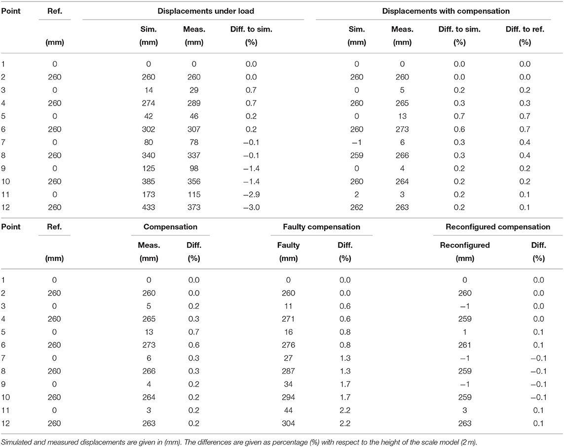
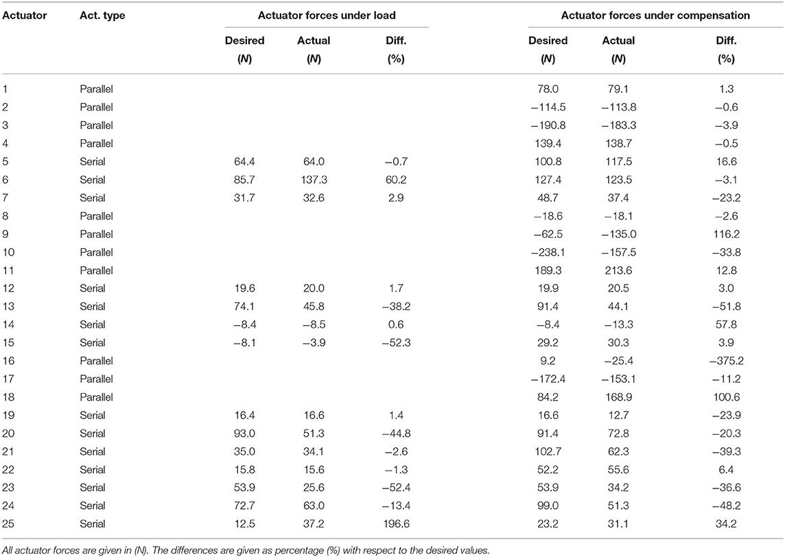
Table A2. Table displaying the data of Figure 8.