Reliability Based Life Cycle Management of Bridge Subjected to Fatigue Damage

Introduction

Every year, transport infrastructure is subject to significant maintenance activities, requiring considerable monetary investment. However, some of the national road network and major elements of the rail infrastructure on the TEN-T network are up to 150 years old and were not designed to modern standards (European Railway Agency, 2014; Gkoumas et al., 2019a). Additionally, due to extreme weather and climate change, many objects are subjected to much higher loading than would have been considered when they were designed (Forzieri et al., 2015). When combined with factors such as population increase, evolution of live load and high-speed vehicles, many structures are currently being loaded beyond their design limit. Most of the bridges built after 1945 are reaching the end of their service life and they are generally in need of major repair or need to be upgraded to a higher functional level (FIEC, 2018). The majority of those bridges are operational today, but some of them are having serious safety problems, which was witnessed with the collapse of the Genoa bridge in Italy in August 2018. The bridge was in service since 1967 and has showed the consequence of major lack of maintenance (New York Times, 2019). Bridge failures lead to closure of sections of the transport network and put excessive strain on already insufficient maintenance budgets.

To avoid new catastrophes, a reflection on life expectancy and maintenance planning is needed. Research and application related to condition assessment, structural health monitoring, prediction models and strengthening techniques are summarized in Denarié et al. (2009); Brühwiler and Denarié (2013); Moreu et al. (2018); Brühwiler (2019); FHWA (2019); Gkoumas et al. (2019b). The European Commission (2019) has also recently released a discussion paper called State of Infrastructure Maintenance, which identifies relevant aspects, namely the state of transport infrastructure and the current practice in planning and execution of monitoring and maintenance technologies, quantification of maintenance backlog, governance structure and the implementation of innovations in all previously mentioned activities. Therefore, the optimization of infrastructure maintenance planning is crucial for road and rail authorities. It is a process of deciding the scope, timing, costs, and benefits of future maintenance activities on a specific asset while taking into account the relative importance of the asset with respect to the overall road or rail network. For over 20 years various Asset Management Systems (AMS) have been used around the world to develop maintenance plans and allocate available budgets (Patidar et al., 2007; ASCAM, 2012; Hurt and Schrock, 2016). These systems typically include condition assessment of assets (mostly based on visual inspections), performance prediction based on historical data and Life Cycle Cost (LCC) analysis (Davis Langdon Management Consulting, 2014). Although useful for allocating budgets for smaller and simple objects, these systems are usually do not include reliability based concepts nor take into account other performance aspects related to economy, society, environment, etc. (Allah Bukhsh et al., 2019). Van Dam et al. (2012) recommended that asset management should no longer be viewed as a solely technical process, but instead should be viewed as a socio-technical process. van der Velde et al. (2013) presented a holistic approach to asset management at highway agency in the Netherlands, which aims to deliver best service to the public at the lowest life cycle cost, given the public acceptance of risk. Nevertheless, one of the main remaining challenges is how to quantify non-technical performance goals and how to link strategic level decision making to performance requirements at an asset level. Therefore, the research presented in this paper aimed to quantify the probability of failure of an asset and the related consequences to the society, which are then both integrated into a reliability based life cycle cost model.

The proposed model is based on the reliability assessment of a bridge suffering from excessive fatigue damage, and integrates traffic flow model outputs in order to determine the impacts of closures or any disruptions caused by construction or maintenance activities on users. This research work is part of the SAFE-10-T project (http://www.safe10tproject.eu/), and has been implemented on a case study of a bridge in the Port of Rotterdam in the Netherlands. The bridge is part of the multi-modal transport network, hosting road, and rail traffic and crossing waterway channel thus presenting a critical node where a failure would have major consequences. Because of its transport significance together with safety and renewal aspects, the bridge was selected as a case study object for the project. During a recent inspection of the road bridge, severe fatigue damage was noted, resulting in the decision to take measures to secure the safety of road users no later than 2020 (Schultz van Haegen, 2017). At the time the Safe-10-T project started, the preparation for the projects where already in an advanced stage. The Safe-10-T project was a study project to see how these sort of decisions can be supported by quantitative life-cycle decision support tooling.

Fatigue is a significant cause of failure in steel bridges subject to cyclical loading over time. There have been a number of recent studies that have used fatigue life as an indicator of structural health in order to inform and update maintenance strategies for steel bridges (Sahrapeyma et al., 2013; Huang et al., 2016; Lee et al., 2017). In Huang et al. (2016), the growth of fatigue cracks in steel bridge members were modeled stochastically with uncertainty using the Gamma process in order to determine the remaining fatigue life of the structure. The effects of maintenance and repair actions were then evaluated by reducing the length of the modeled cracks. In Sahrapeyma et al. (2013), a probabilistic approach is used to create a profile of the reliability index of a steel bridge and a numerical approach is used to determine the effects of different maintenance and repair actions over time. In Lee et al. (2017), a method of performing a probabilistic fatigue assessment of a steel railway bridge is presented that may then be updated using the results of inspections or repair actions in order to inform future maintenance needs.

In general, prediction of the fatigue life of steel bridges is performed using either the S-N curve method or by a more involved fracture mechanics approach. Often the S-N approach is used at the design or preliminary assessment stage, while the fracture mechanics approach is used for more refined assessment of remaining fatigue life or inspection and repair estimates (Chryssanthopoulos and Righiniotis, 2006). The S-N curve approach relates the constant-amplitude cyclic loading applied to a fatigue detail to the number of load cycles that can be applied before failure of that detail. This approach is adopted by a number of design standards (BSI, 1980; AASHTO, 1990; CEN, 1992). When combined with Miner's rule (Miner, 1945), this may be extended to include loading with varying amplitude. This results in the ability to calculate the cumulative fatigue damage effects of non-uniform load cycles, such as typical traffic loading on a bridge. However, typically this method does not account for crack growth or model uncertainty. Various probabilistic methods have been presented in literature in order to adapt the S-N method and allow for more accurate prediction models (Kwon and Frangopol, 2010; Kwon et al., 2012; Adasooriya, 2016). This study combines long-run loading simulations based on WIM data, fracture data from inspection reports and probabilistic methods in order to obtain a comprehensive picture of the reliability profile of the bridge at the fatigue limit state. Model updating is then used to present the effects of several maintenance scenarios to inform a life-cycle cost model.

The goal of the proposed long term bridge management strategy is to determine the optimal maintenance scenario, which is based on reliability assessment and takes into account the economic, societal, and environmental impacts of planned and unplanned (e.g., hazards, failures) maintenance interventions. The aim is to develop maintenance strategies which will provide more reliable, available, maintainable, safe, and cost-efficient infrastructure.

Case Study Description

Introduction

The port of Rotterdam is the largest port in Europe with a throughput of 467.4 million tons, including dry bulk, liquid bulk, and containers. A severe disruption at the port is expected to have significant impact on freight traffic through Europe. The newest and largest container terminals can be found at the Maasvlakte, see Figure 1 (Port of Rotterdam Authority, 2019). Goods are transported to and from Rotterdam via sea, inland waterways, rail, roads, and pipelines throughout Europe. The port's ambition for 2033 is to reach a modal split of 20% rail, 35% road, and 45% inland waterway traffic for the Maasvlakte (Pastori, 2015).

FIGURE 1

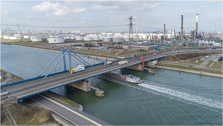
Figure 1. View on the selected bridge for the case study in the Port of Rotterdam (Port of Rotterdam Authority, 2019).

A critical highway and rail bridge to connect the Port of Rotterdam to the inland has been selected as a case study for this work (i.e., for rail it provides the only connection, for road one detour across a secondary road is available), its' impact on multiple transport modes, and its usage by both passenger and freight user groups (European Commission, 2018). Furthermore, the influence of a potential bridge failure is significant, affecting not only national but also international traffic across the TEN-T corridors. Additionally, its recent degradation and renovation plans make it an interesting object for both reliability assessment and life cycle analysis.

The bridge was built in 1972 and it provides a road and rail connection from the port toward the hinterland. The road bridge is a part of the highway network, consisting of two lanes per direction (plus a walking/cycling path), while the railway bridge consists of two tracks (one per direction). Besides that, multiple ships pass under the bridge daily in order to reach part of the Europoort and part of the more Westerly harbors in Rotterdam. Although the road and rail bridge have shared foundations, each superstructure is entirely independent. The road bridge is the primary focus of this study and is a four-span steel girder structure. The bridge deck is constructed with a steel plate stiffened by longitudinal troughs. The troughs span between transverse cross girders, which span between two longitudinal girders. The cross girders also have a cantilever on each side of the bridge, as presented in typical cross section in Figure 2. The lengths of the four continuous road bridge spans are 55, 95, 41, and 41 m, moving from south to north. The 55 and 95m spans are continuous, while the first 41 m span is a bascule structure (Rijkswaterstaat, 2016).

FIGURE 2

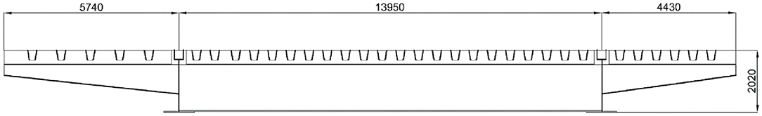
Figure 2. Typical cross section of the orthotropic steel deck, dimensions in mm.

Inspections have shown the road bridge to be experiencing serious deterioration due to fatigue, indicating that an upgrade of the structural performance would be required in order to guarantee safety in the future. An intensive crack monitoring and repair measures were taken from that moment on. The final rehabilitation solution, now under construction, was strongly influenced by future uncertainties related to functional changes in the road and rail track, but also the possible effects of sea water rising and climate change. Because it was not possible to wait any longer, a temporary bridge was chosen. Safe-10-T has looked on if and how Whole Life Cycle Cost Model (WLCCM) could have contributed in decision processes, and how this could have helped to provide insight on the actual impacts on risks, cost and societal effects of different rehabilitation scenario's. The results will not change the chosen solution for this bridge, but does make a great showcase for similar situations in the future.

Degradation Problems

During regular inspections, several steel cracks were detected in the orthotropic bridge deck in 2006. These were concluded to be caused by fatigue damage. Following this, a plan was put forward by the owners to renovate the bridge using high-strength concrete: a method used often within the Dutch bridge renovation programme. The aim was to extend the life of the bridge by 30 years. However, this particular bridge wasn't found to be suitable for this renovation method, as the troughs are not continuous over the cross girders. Due to the continuously increasing traffic intensity, the evolution of cracks has continued. Thus, the bridge is being monitored and the cracks are regularly welded. In addition, it was decided in 2016 that the bascule part of the bridge should no longer be opened for safety reasons. Currently, ships higher than 11.5 m cannot follow the Hartelkanaal due to this closure. To ensure ongoing safety, an intense inspection program was set-up, including inspections every 3 months. It was estimated that by 2020 the live load on the bridge would have to be drastically decreased to ensure safety if no major rehabilitation measures would have been taken. Therefore, the owners decided to build a “temporary” bridge adjacent to the current bridge. The tender was awarded in 2019, and execution works have started in 2020. The bridge will serve one-way traffic from the Maasvlakte toward Rotterdam for at least 10 years, and is planned to be in service by 2022. The main bridge itself will continue to be used for one-way traffic until 2030. Traffic loads will be set to the center of the bridge, currently least affected by degradation (Rijkswaterstaat, 2016; van der Tuin et al., 2020).

Reliability Model

In order to determine the current condition of the structure, reliability-based engineering methods were required. This involves modeling the inputs to the assessment stochastically (i.e., as random variables, having an associated uncertainty). The result of the analysis is that bridge safety can be considered in terms of failure probability, allowing calculation of the associated risk.

Determination of the Critical Limit State

The case-study bridge undergoes regular inspections in order to identify and monitor damage locations throughout the structure. From the resulting inspection reports, it may be concluded that the key issue facing the bridge is cracking due to fatigue. The most recent bridge inspection report showed 196 no. individual cracks throughout the bridge. Of this number, 16 no. had initiated since the last inspection in the previous year and 180 no. were pre-existing. Of the existing cracks 36 no. had increased in length since the previous inspection 1 year before. Fatigue damage is a common issue in steel orthotropic decks, which for the current structure has been aggravated by the significant traffic growth since the bridge was designed, including increasing amounts of freight. Calculation of the reliability of the structure was required with respect to the Fatigue Limit State (FLS).

The bridge owners have indicated areas on the bridge that have been deemed “critical” due to their location at the bridge supports. In the most recent bridge inspection, a crack was noted at one of these critical locations that had not been present in previous inspections. This crack was found at the connection between the cross girder and the trough stiffener near the northmost bridge pier. The crack had a length of 220 mm at time of inspection, indicating that 220 mm of propagation had occurred since the previous inspection in 2017. According to the results presented in the most recent inspection report of 2018, this indicates that this is the fastest rate of crack propagation at present. The nature of this crack is that it initiated at the trough bend and propagated upwards along the weld toward the deck plate (see Figure 3).

FIGURE 3

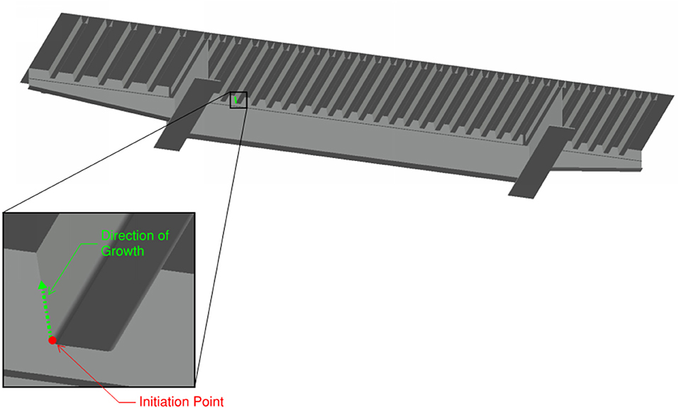
Figure 3. Location of “critical crack” modeled probabilistically (highlighted in red).

In order to comprehensively model the failure probability of the entire system, it would be necessary to model each existing crack, as well as to predict the locations of future damage and account for these also. According to Melchers and Beck (2018), the failure probability for any structural system may be defined within the bounds shown in the equation (Equation 1) below.

$\begin{array}{ll}1-{\displaystyle \prod _{i=1}^n}\left[1-P(F_i)\right]\ge P(F)\ge max\left[P(F_i)\right]& (1)\end{array}$

Where:

P(F) is the probability of failure of the system

n is the total number of fully dependent elements in the system

P(F_i) is the probability of failure of the ith element.

This essentially means that the actual probability of failure of the system lies between the failure probability of a fully dependent and fully independent system. It can be seen from the inequality that the more conservative bound involves the consideration of a fully dependent system, whereas considering the system elements to be entirely independent results in a less conservative probability of failure (PoF).

In reality, there is a degree of inter-dependency between damage locations, where damage at a particular point can lead to changes in the stress distribution through the structure and induce damage at a secondary point. The relative failure probability of multiple elements is also a factor to be considered when evaluating inter-dependency. It can be seen in Melchers and Beck (2018) that inclusion of failure modes that are significantly lower than the primary mode of failure has negligible impact on the failure probability of the system when compared to the consideration of the system as completely independent. Given the number of cracks apparent on the bridge, it was determined that the most efficient method of calculating the system failure probability is to model a single, most critical crack as an independent entity as opposed to considering system dependencies. This means that for this case, it was assumed that the overall failure of the system is defined by the probability of failure of a single critical crack (i.e., the maximum probability of failure of a fully independent system). The chosen critical point was the crack located between the connection of the trough to the cross girder, mentioned previously. This crack was chosen due to its perceived “critical” location at a support point of the bridge, as well as the speed of crack propagation which indicates a very high failure probability that will govern the system failure.

Probabilistic Fatigue Analysis

Fatigue in bridges can be defined as the weakening of the structural material caused by cyclic loading due to vehicle passages that results in progressive and localized structural damage and the growth of cracks. In a traditional deterministic fatigue assessment, the number of cycles at various stress ranges are estimated or calculated on the basis of Structural Health Monitoring data. The number of cycles at each stress range is then divided by the capacity for the fatigue detail (and stress range) and summed in order to calculate the damage factor (D). In order to obtain the failure probability at the Fatigue Limit State (FLS), a probabilistic fatigue assessment methodology was developed. Within this procedure, stress signals can be obtained either from strain gauge measurement, or by running live load models (or measured live loads) over influence lines pertaining to hot spots on the bridge. Rain flow counting algorithms are then used to calculate a stress range histogram for the fatigue detail. The performance function considered for probabilistic fatigue assessment is given by:

$\begin{array}{ll}g(x)\le 0& (2)\end{array}$

Where:

$\begin{array}{ll}g(x)=D_{crit}-{\displaystyle \sum _{i=1}^n}\frac{n_{Ei}}{N_{Ri}}& (3)\end{array}$

In the above equation (3), D_crit is the critical damage factor, modeled as a lognormal distributed variable with mean and standard deviation equal to 1.0 and 0.3 as recommended in the literature (JCSS, 2001). The procedure for determining a stochastic interpretation for n_Ei is illustrated in Figure 4. After calculating the stress range histogram for each year, uncertainty and Dynamic Amplification Factors (DAFs) are applied to each bin separately. Once a bin has been multiplied by the distribution for uncertainty and DAF, the final distribution for that stress range is sampled 100,000 times. Once this has been done for each bin, the resulting stress ranges can once again be binned in a matrix containing 100,000 samples of a 100-bin histogram. The result is a probabilistic representation of n_Ei. A probabilistic S-N curve is then used to determine a stochastic representation of N_Ri for each stress range, Δσ_i. In the absence of existing research pertaining to probabilistic consideration of the Eurocode S-N curves, the Det Norske Veritas (2010) S-N curves are used.

FIGURE 4

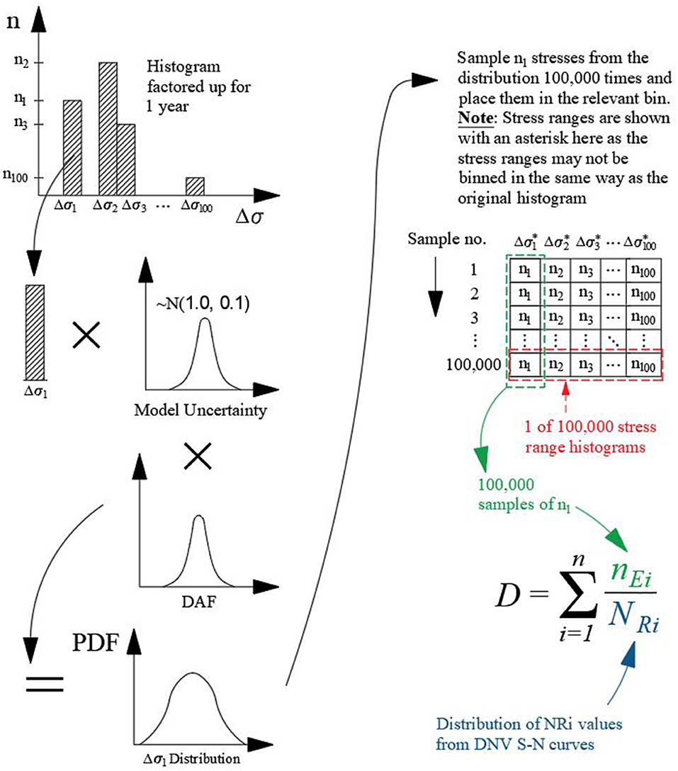
Figure 4. Probabilistic Fatigue Assessment Methodology.

Finite Element Modeling

In order to obtain stress signals for the fatigue analysis, live loads were run over influence lines extracted from a Finite Element (FE) model. As mentioned previously, the critical limit state being assessed was fatigue cracking between the web of the troughs and the cross girder. This cracking is due to axial stress in the trough at the interface (Det Norske Veritas, 2010). In order to obtain this “hot-spot” stress, and to enable modeling of growth in crack length, a multi-scale FE model was required. The model is illustrated in Figure 5, with the deck plate omitted for clarity. The model was developed in the MIDAS FEA and MIDAS Civil commercial software, using a combination of beam and plate elements. The locations closer to the “hot-spot” were modeled with a dense plate mesh, to enable refined analysis and output. The dense mesh was chosen for this model with an irregular discretization of plate elements. The discretization pattern was chosen to allow reading of results at the relevant points. Additionally, the mesh size was reduced as to as small a size as practicable, in order to ensure accurate local modeling while also optimizing the computational cost of the analysis. The local model results were verified by comparison to a global beam model.

FIGURE 5

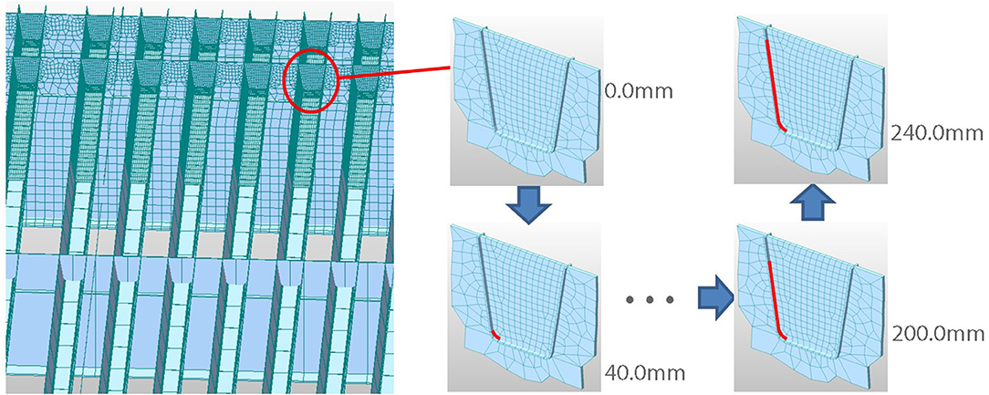
Figure 5. Multi-Scale FE modeling and crack propagation.

In order to investigate the implication of crack growth on the stress concentration, nodes were periodically removed to account for the scenario where fixity is no longer available, due to fatigue failure. This allows failures with varying consequences to be modeled in the analysis. Due to the computationally intensive nature running a 3D FE model, it was not possible to run moving loads over the model. For this reason, influence lines were extracted from the model by placing unit forces along the locations of the vehicular wheel loads. These influence lines were then extracted to MATLAB, where live loads from trucks over time could be run over the stress influence lines, to obtain stress signals. It should be noted that when applying wheel loads to the generated influence lines, each wheel load was considered as a pressure represented by the wheel force divided by the contact area of the deck. The contact area was given by the contact area of the wheel. An additional allowance was made for the increase in the distribution area as the load is dispersed through the deck surfacing, in accordance with EN 1991-2 (2003).

In order to calibrate the FE model, the previous inspection reports were used. The crack being modeled in detail here was found to begin in 2018, and grew rapidly to a 220 mm crack by 2019. Therefore, the stress concentration factors in the fatigue analysis were calibrated in order to produce a 10% probability of obtaining a 40 mm crack in 2017, and a 10% probability of obtaining a 220 mm crack in 2019.

Live Load Modeling

In order to perform the probabilistic fatigue analysis, loading information is required for the time of construction of the bridge, through its current age and up to the end of the assessment period. This is of course impossible to obtain. For this reason, a long-run-simulation methodology was employed. The first step was to obtain Weigh-In-Motion (WIM) data representative of the bridge in question. For this purpose, 6 months of the most recent WIM data was gathered from the closest available WIM site to the bridge. The data was first screened and cleaned according to the rules developed in Hajializadeh et al. (2015).

Probabilistic distributions were then fitted to the traffic. Multimodal normal distributions were fitted to the data pertaining to Gross Vehicle Weight (GVW), allowing both full and empty trucks to be simulated, while also allowing extrapolation of potentially heavier vehicles than those measured in the WIM data. Empirical distributions were fitted to the vehicle gaps and inter-axle spacings. The simulation technique can be used to model same-directional, two lane traffic. Previous research (O'Brien and Enright, 2011) noted a correlation in the weight of vehicles in overtaking events, which can have a significant impact on bridge load effects. For this reason, O'Brien and Enright (2011) employed a scenario modeling approach which maintains this correlation in the simulated data. This methodology is not conducive to modeling of traffic growth or changes, due to the lack of probabilistic modeling of the traffic. Therefore, in the SAFE-10-T project, correlated multimodal weight distributions were used to consider these inter-lane correlations within the Monte Carlo Long-Run Simulation approach described. The approach allows consideration of both past and future changes in traffic weight and frequency.

In order to simulate the correct number of trucks per day, the vehicle counts throughout the assessment period were required. Traffic counts from 1972 to the present date were based on historic figures provided by the Port of Rotterdam on freight vehicles passing over the bridge. Traffic counts from 2018 for both directions were obtained from the bridge owners (Port of Rotterdam, 2018). Future daily traffic counts were based on traffic growth predictions as described in section Impact on the Traffic Flow.

The influence line for the fatigue detail in question was such that no two vehicles would impact the detail within the same lane at any one time. Therefore, the intervehicle gaps in the slow lanes (in seconds) was assigned based on the number of seconds in a day, divided by the number of vehicles per day(n_veh), as per the equation (Equation 4) below:

$\begin{array}{ll}Gap[s]=\frac{86400}{n_{veh}-1}& (4)\end{array}$

Finally, overtaking events were simulated by firstly investigating the percentage of fast-lane vehicles that were participating in an overtaking event (i.e., where the inter-lane gap was 1.2 s or less) in the WIM data for both directions. This percentage was calculated for both weekends and weekdays. The instances of overtaking events in the WIM data were collated and an empirical distribution was fit to all overtaking time gaps for each direction. Inter-lane time gaps for the overtaking events could then be sampled from this empirical distribution and applied relative to selected slow-lane vehicles. The slow-lane participants for these events were chosen at random. Once these vehicles had been selected, the closest fast-lane vehicle was found and its position was altered to represent the sampled inter-lane gap.

The outcome of the live load modeling was a load model for the bridge in question from the time of construction up to 2040, which can be related to the traffic growth scenarios described in section Impact on the Traffic Flow.

Life Cycle Management Scenarios

For the selected case study, four life cycle management scenarios have been analyzed, which take into account the existing road bridge, construction of a temporary bridge, and construction of a new bridge. At the time of writing, the condition of the rail bridge is considered sufficient, and therefore it will not be analyzed in great detail. However, the multimodal influence regarding traffic flows and mode switches is taken into consideration within the traffic flow model. The following management scenarios have been defined within the case study:

1. A “do minimum” scenario where the condition is maintained with regular inspections and welding of newly occurring fatigue cracks. The bridge is not improved or replaced by a temporary bridge until the new bridge is constructed.

2. An “additional maintenance” scenario where several options of improving and strengthening the bridge are analyzed, including the new probabilities of failure.

3. The “temporary bridge” scenario, representing the current plans of the agency, where a temporary bridge will be built next to the existing bridge and will remain in service for the next 10 years.

4. The “new bridge” is built as soon as possible and the existing bridge is decommissioned now.

Impact on Reliability Level

For each of the management scenarios considered, welding is always assumed to occur in 2019, as this is known to have taken place on the modeled crack. In order to model the effect of repairing the weld, the nodes which are removed in the “cracked bridge” model are repaired, and the associated stress history is re-set. Figure 6 illustrates the failure probability over time from the beginning of the fatigue life of the bridge up to the end of the assessment period, for various crack lengths. After 2019, the failure probability for a 240 mm is only slightly less than that of a 40 mm crack. This is due to the nature of the traffic growth. Should a 40 mm crack occur in a year, the model shows that it is very likely that this develops into a longer crack before the next year.

FIGURE 6

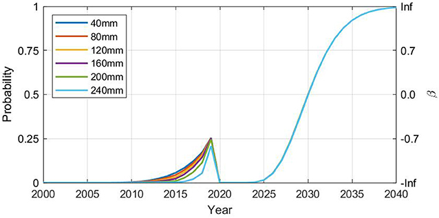
Figure 6. Variation in crack length probability and reliability over time (welding in 2019).

The reliability index (β) is also shown on the Y-axis in Figure 6. β is a standard measure used to describe the safety of structural systems, and is related to the failure probability (P_f) by Equation (5):

$\begin{array}{ll}\beta ={\Phi }^{-1}(P_f)& (5)\end{array}$

Where:

Φ⁻¹ is the standard normal inverse function.

It should be noted that the tick labels shown in Figure 6 on the secondary vertical axis for β only correspond to the opposite failure probability on the primary vertical axis (i.e., the axis is not to scale). The β-values are only shown for the purposes of scaling against failure probabilities. In 2019, when the probability of various crack lengths reached around 0.25, the β-values reached around 0.7. ISO 2394 (2015) recommends a target (minimum) reliability index of 2.3 for fatigue, depending on the possibility of inspection. It can also be seen that should no more maintenance action be taken within the assessment period, the situation will rapidly deteriorate beyond anything which has been previously foreseen.

Scenario 1: “Do Minimum”

In order to model the first management scenario, welding is built into the FE model as per the 2019 situation every time the reliability drops below 2.3 (as recommended by ISO 2394). Although it is possible to investigate the impact of basing the reliability on various crack lengths (and various associated risks), for this analysis it is clear that the best strategy is to base the repair on the occurrence of a 40 mm crack, as longer cracks have similar probabilities (Figure 7). It was calculated that in order to keep the reliability above 2.3, welding would be required in 2024, 2029, 2034, and 2038.

FIGURE 7

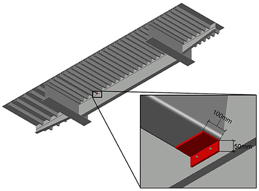
Figure 7. “Additional maintenance” option 1 – angle stiffener.

Scenario 2: “Additional Maintenance”

An investigation was carried out into major intervention works that could strengthen the existing bridge. The aim of these works was to reduce the axial stress in the trough at the welded connection with the cross girder which would reduce the likelihood of cracking. This would lead to an increase in the fatigue life of the connection. The primary forms of major intervention “strengthening” investigated for the case study bridge were:

1. Stiffening of the connection using a steel angle bolted to the cross girder below the existing welded trough connection. This method is currently employed by the bridge owner to strengthen this type of crack. The angle is welded to the bottom flange of the trough and bolted to the cross girder with prestressed bolts, as shown in Figure 7. The effect of the angle in the FE model was considered by connecting a plate element to the bottom flange of the trough along the weld seam with rigid links, as well as at the bolts location.

2. Stiffening of the existing trough members using an Ultra High Modulus (UHM) Carbon Fibre-Reinforced Polymer (CFRP) strip bonded with the base of the troughs, as shown in Figure 8. An off-the-shelf design was investigated consisting of a 2.5 mm thick CFRP strip with a stiffness of 360 MPa. In order to model the effect of the FRP, a plate element with this thickness was attached to the bottom of the trough in the FE model with rigid links. The stiffness of the element in the FE model was reduced by 7% in order to account for the flexibility of the adhesive layer, as recommended by Moy and Bloodworth (2007). The CFRP was applied over a 2.25 m length close to the cross-girder connection.

FIGURE 8

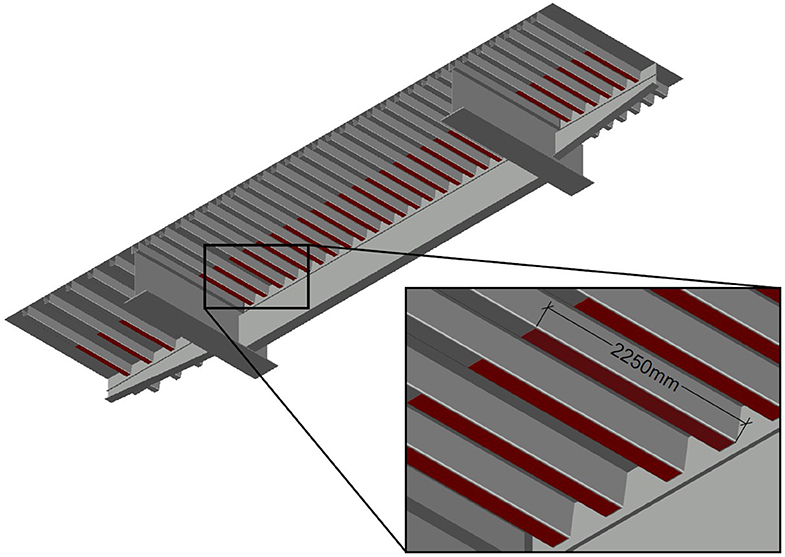
Figure 8. “Additional maintenance” option 2 – FRP Strips.

It was assumed that at the time when each strategy is put in place, the connection will be rewelded. Each repair strategy will have varying costs associated with implementation, as well as having different effects on strength increase. The FRP binding is clearly preferable from the perspective of installation. Additionally, the analysis showed that the FRP strategy would result in a maximum stress reduction of around 23% per axle, while the steel angle strategy would result in a stress reduction of less than 7%. For this reason, only the FRP strategy will be addressed in detail in this work.

Scenario 3: “Temporary Bridge”

The temporary bridge scenario will be modeled as per the current plan of the bridge owner. The temporary bridge will be assumed to be in place in 2024, when the reliability drops below 2.3. Within this scenario, the two central lanes of the existing bridge remain open to traffic in one direction, as these areas are currently the least damaged, see Figure 9. In this case, the reliability (and failure probability) of the system is governed by the most severely stressed trough-cross girder connection beneath the two central lanes of the existing bridge. The temporary bridge will be assumed to be designed to safely carry the required traffic for 10 years. In order to perform the analysis, the load history and failure probabilities up to the year 2024 must first be calculated for the new critical fatigue detail.

FIGURE 9

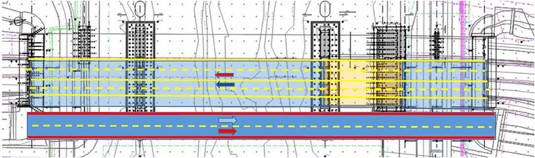
Figure 9. Plan view of traffic lanes over existing bridge and temporary bridge.

Scenario 4: “New Bridge”

In order to model the maintenance scenario of a new bridge, it is assumed that the new bridge is put in place in 2024, prior to the reliability dropping below 2.3. The new bridge is assumed to have a β-value of 5.2 (failure probability of 10⁻⁷) for the duration of the maintenance period, assuming that all newly designed fatigue details will survive a 120-year life.

The results of each maintenance strategy can be seen in Figure 10 below, in terms of the change in failure probability over time, for a 40 mm crack. It can be seen in the figure that each scenario has the same profile of failure probability until 2025, since each strategy consists of welding the existing bridge up to this point. Scenario 2, “additional maintenance,” is indicated by the solid yellow line, and it can be seen that after welding and FRP is put in place in 2024, the failure probability does not begin to deteriorate rapidly until 2033 when the weld begins to succumb to fatigue failure, despite the stress reductions offered by the FRP. Scenario 3, “temporary bridge,” is indicated by the dotted red line. It can be seen that despite the temporary bridge being put in place in 2024, the critical weld begins to deteriorate rapidly in around 2027.

FIGURE 10

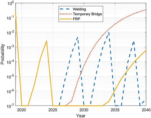
Figure 10. Change in probability of failure in time for different scenarios.

Impact on the Traffic Flow

For each of the maintenance scenarios, different traffic regulations will be in place and therefore different traffic flow impacts will occur. In order to determine the consequences on the traffic the following parameters were considered: the duration of the closure, the type of traffic regulation during the maintenance and the traffic capacity. According to the existing regulation practice and required maintenance activities, they will result in six different closure-types (van der Tuin et al., 2020):

• Closure of roads underneath bridge

• Closure of all lanes on the east side

• Speed limit of 70 km/h on the west side

• Closure of all lanes on the west side

• Speed limit of 70 km/h on the east side

• Closure one lane per direction

• Speed limit 70 km/h on each side

• Full closure

The SAFE-10-T transport model can model multimodal transport for both freight and passenger traffic, while incorporating effects of disruptions which are varying over time. The transport model is based on the well-known 4-step passenger (Ortúzar and Willumsen, 2011) and 5-step freight transport models (Tavasszy, 2006). To simulate the dynamics of user behavior during disruptions correctly, the model consists of two separate models: a Local Disruption model (LD) which simulates the region in the vicinity of the affected object using dynamic traffic assignment, and a Global Spill-over model (GS) employing static traffic assignment to be able to propagate disruption effects for long-distance transport. The general order of running both models is: first delays are computed for the LD model, followed by running the GS model (incorporating output of the LD model). In the model we assume that disruptions only directly affect traffic in the vicinity of the infrastructure object. As such, trip cancellations, modal shifts and departure time changes are only modeled at the detailed level based on available data about traffic quantities. The resulting delays and choices made are incorporated in the GS model. More details can be found in van der Tuin and Pel (2019). The local disruption model uses a dynamic traffic assignment, whereas the Global Spill-over model employs a static traffic assignment on the network of Europe. The future scenarios are based on two factors: global economic growth and energy transition, which resulted in four future traffic scenarios, as shown in Figure 11A:

• Conservative Carbon: Low economic growth due to limited international collaboration. Oil stays dominant, resulting in high energy prices.

• Fossil forward: International trust leads to a rapid growth in world trade. Still reliant on fossil fuels, but there does exist a focus on cleaner production and limited usage.

• Lean & Green: Low economic growth results in a lower demand on energy. Renewable energy sources are stimulated but stay expensive and require subsidies from government.

• Green Unlimited: An international approach stimulates radical changes in renewable energy, leading to a fast energy transition. International trust and collaboration leads to a high economic growth.

FIGURE 11

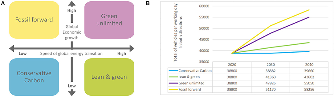
Figure 11. (A) Overview of the four future traffic scenarios and (B) predicted number of vehicles for analyzed bridge in 2020, 2030, and 2040 (van der Tuin and Pel, 2019).

In general, it is expected that a higher speed of energy transition results in less volumes transported (crude oil, coal, related products). Combined with low economic growth this is expected to result in less or stabilized total traffic flows for the Conservative Carbon, Green Unlimited and Lean & Green scenarios (Port of Rotterdam, 2018; Port of Rotterdam Authority, 2019). The traffic in the studied area mainly consists of containerized traffic, and therefore is less affected by a high speed of transition toward renewable energy. For the calculation of life cycle maintenance scenarios, this paper assumes Business as usual/Conservative Carbon traffic will continue for a period of 100 years. Traffic scenarios are developed for 2020, 2030, and 2040—each having a different expected amount of traffic, as shown in Figure 11B. Further details on traffic flow model can be found in van der Tuin and Pel (2019).

Whole Life Cycle Cost Model

The main objective of the Whole Life Cycle Cost Model (WLCCM) is to determine direct and indirect impacts of planned and unplanned disruptions. Different investment scenarios are evaluated based on the impacts of each alternative and its associated activities. The developed model takes into account the consequences of different maintenance interventions in terms of economy effects for the agency, impacts on the users calculated as user delays caused by traffic regulations and impacts on the environment caused by usage of materials and traffic congestion (Stipanovic et al., 2017; Skaric Palic and Stipanovic, 2019).

Different life cycle cases consisting of the scenarios described in section Life Cycle Management Scenarios are analyzed within the model. The timing of a certain scenario is based upon the reliability assessment and is triggered when a threshold reliability index is reached. The processes involved in the life cycle analysis and the structure of the WLCCM model are shown in Figure 12. In the next paragraphs quantification of cost components are explained in detail.

FIGURE 12

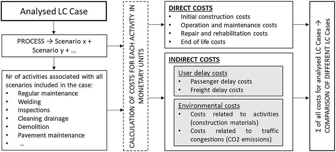
Figure 12. Structure of the Whole Life Cycle Cost Model (Skaric Palic and Stipanovic, 2019).

Construction Costs

The direct construction costs are calculated by dividing the designed object into separate construction elements. The unit cost of each element is obtained and multiplied by the number of occurrences in the design. This results in the total costs of an element in the total object. Doing this for every element and summing these costs will yield the total assigned construction cost.

The rest of the initial construction costs are calculated by taking a percentage of the direct construction costs (plus the one-off, execution and general costs, if applicable). The percentage (and represented value) should be based on the statistical data of the owner. All these costs are incurred at the beginning of the life cycle of the object. Therefore, there is no need for any discounting. The calculation of the initial construction costs are therefore given by Equation (6):

$\begin{array}{ll}ICC={\displaystyle \sum _{i=1}^n}{CUC}_i\times {Cq}_i\times (1+\chi )& (6)\end{array}$

wherein

ICC = initial construction costs (€)

i = construction element from element 1 until element n

CUCi = construction unit cost of element i (€/unit)

Cqi = the quantity of construction element i present in the design (unit)

x = an additional percentage to cover unassigned, indirect, engineering and other costs.

Maintenance Costs

The maintenance costs are calculated in a similar manner to the initial construction costs. First the maintenance scenario that most accurately describes the estimated required maintenance over the life cycle of the object is determined. This requires determination of the various necessary maintenance activities, their accompanying frequencies and their estimated unit costs. Next, the unit cost of a certain maintenance activity (AUCi) is multiplied by the quantity of units related to that activity (Aqi). The yearly maintenance cost for that activity is then attributed to all the years in the life cycle of the object in which that maintenance activity takes place (based on the frequency attributed to that activity). This creates a maintenance schedule for which the total maintenance costs of every year in the life cycle can be calculated.

The maintenance costs for one specific year are therefore calculated by Equation (7):

$\begin{array}{ll}{MC}_{t,nom}={\displaystyle \sum _{i=1}^n}{AUC}_i\times {Aq}_i& (7)\end{array}$

Wherein:

MC_t, _nom = nominal maintenance costs for year t (€)

i = activity 1 until n

AUC_i = unit cost of activity i (€/unit)

Aq_i = quantity of units for activity i in year t (unit).

Summing the maintenance costs of each year in the life cycle of the object gives the total nominal maintenance costs of the object. Because the maintenance costs are made in the year the maintenance takes place, the future cash flows must be discounted to create a present value.

The total discounted maintenance costs may be increased by a certain percentage to cover the unassigned costs, indirect costs and unassigned object risks (but not engineering costs and other additional costs), if that is the owner's practice.

The total maintenance costs for the object during its life cycle is therefore calculated by Equation (8):

$\begin{array}{ll}{MC}_{tot,disc}={\displaystyle \sum _{t=0}^T}\frac{{MC}_{t,nom}}{{(1+r)}^t}\times (1+\chi )& (8)\end{array}$

Wherein:

MC_tot = the total maintenance costs during the life cycle of the object (€)

MC_{t, nom} = maintenance costs for year t (€)

t = year in life cycle from 0 until end of life cycle T

r = the discount factor (%)

x = an additional percentage to cover unassigned, indirect, engineering, and other costs.

End-of-Life Costs

The third subcategory in the category agency costs are the end-of-life costs. These include the costs of demolition and disposal minus the residual value. In this model the end-of-life costs will be calculated in the same way that the initial construction costs are calculated. Namely by assigning the construction elements with a unit cost for end-of-life costs and multiplying the amount each building element with the corresponding end-of-life unit cost. In this research it will be assumed that the residual value is equal to zero. The resulting equation (Equation 9) is given by:

$\begin{array}{ll}{EoLC}_{nom}={\displaystyle \sum _{i=1}^n}{DUC}_i\times {Cq}_i& (9)\end{array}$

Wherein:

EoLC_nom = nominal end-of-life costs (€)

i = construction element from element 1 until element m

DUC_i = demolition and disposal unit cost for element i (€/unit)

Cq_i = the quantity of construction element i present in the design (unit).

Because the end-of-life costs take place at the end of the life cycle of the object the costs must be discounted in Equation (10). This is done as follows:

$\begin{array}{ll}{EoLC}_{disc}=\frac{{EoLC}_{T,nom}}{{(1+r)}^T}& (10)\end{array}$

Wherein:

EoLC_disc = the discounted end-of-life costs (€)

EoLC_{T, nom} = the nominal end-of-life costs at the end of the life cycle (€)

T = the year in which the life cycle ends

r = discount factor (%).

User Delay Costs

The equations used for determining the Traffic Delay Cost (TDC) are based on the work of Sundquist and Karoumi (2012). The total user costs are a summation of the two sub-categories; freight delay costs and passenger delay costs. Because the user costs are made during the life cycle of the bridge, future cash flows must be discounted to determine a total present value.

The total discounted user delay costs are determined as follows (11):

$\begin{array}{ll}{UDC}_{tot,disc}={\displaystyle \sum _{t=0}^T}\frac{{TDC}_{fr,t,nom}}{{(1+r)}^t}+{\displaystyle \sum _{t=0}^T}\frac{{TDC}_{car,t,nom}}{{(1+r)}^t}& (11)\end{array}$

Wherein:

UDC_tot, _disc = total discounted user delay costs (€)

t = year in the life cycle from 0 until the end of the life cycle T

r = discount factor (%)

TDC_{fr, t}, _nom = nominal freight traffic delay costs in year t (€)

TDC_{car, t}, _nom = nominal commuter traffic delay costs in year t (€).

The traffic delay costs represent the valuable time of the network users. The economic value of the user's time is dependent on several factors. The type of traffic (passenger vehicle or freight traffic), the amount of persons/cargo per vehicle and the type of cargo/person (business/leisure). The input data for the calculation of traffic delay costs come from the SAFE-10-T multi modal traffic flow model (van der Tuin and Pel, 2019). The transport model computes user delays and traffic flows resulting from a disruption (different maintenance activities to complete bridge failure), incorporating both direct effects (i.e., congestion) as well as secondary effects such as trip cancellations and mode changes. The traffic model gives the values for additional travel time per traffic regulation, depending on the traffic disruptions for two groups of users, namely freight and passengers traffic. Each maintenance activity is associated with a certain traffic regulation which combined with the total activity duration gives additional travel time for total duration of a certain activity. A different value of time is then used for each group of users, based on the literature.

All activities on a bridge are assigned for each year in the developed life cycle cost model. With the previously described methodology for calculation of additional travel time for each activity the traffic delay costs can be then determined by Equation (12) for the analyzed time interval:

$\begin{array}{ll}{TDC}_t=ETT\times {ADT}_t\times VOT\times N_t& (12)\end{array}$

Wherein:

TDC_t = traffic delay costs for year t (€), calculated separately for freight and for passenger cars,

ETT = extra travel time per type of user (hours)

ADT_t = the average daily traffic (quantified separately for freight and for passenger cars) in year t passing the analyzed section or bridge in question (passenger car equivalent PCE/day)

VOT = a monetary value for the user's time (€/hour)—a different value is used for freight and for commuters in this analysis, namely 9.92 EUR for commuting passengers in the car, and 49.57 EUR for freight traffic (de Jong, 2013)

N_t = the duration of a certain maintenance activity (days).

Environmental Costs

Environmental costs represent monetised value of environmental impacts of different activities during the bridge life cycle. The impact on the environment is caused mostly by the materials production and transport during the construction process, maintenance activities, and at the end of a service life of an element or bridge as a whole. According to the environmental study of different bridges presented in Hegger and de Graaf (2013), most of the environmental impacts are caused due to the use of construction material during initial construction and the subsequent maintenance. Therefore, only the effect on the environment per kg per material produced for a certain maintenance activity is considered in this estimation of the environmental costs.

The determination of environmental costs due to maintenance activity is based on three aspects. First, the environmental effect per impact category (EE_i) based on material type is determined using GaBi software database (Thinkstep, 2015). Second, the material quantity per kg produced for the maintenance activity is estimated (M_qj). Finally, to monetise environmental effect into Euros, the environmental effect per impact category values are multiplied by their shadow prices (SP_i) established by de Bruyn et al. (2010).

The environmental impacts per kg of material j for impact category i are given in Table 1. These have been determined with the help of the LCA software GaBi or other literature sources. For the analysis quantity of all materials used for a certain activity is calculated (e.g., quantity of concrete, steel, asphalt etc., needed for construction of a new bridge). Quantity of a certain material is multiplied with the environmental impact per 1 kg, given in Table 1. This is performed for all materials used for a certain activity resulting in environmental impact of a certain activity per impact categories. To enable addition of all impact categories and monetization of the overall environmental impact price for each category is introduced.

TABLE 1

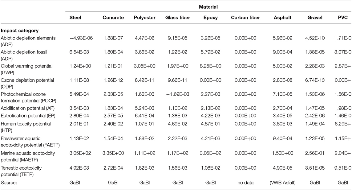
Table 1. Environmental impacts per 1 kg of construction material.

Table 2 presents the environmental effect categories along with their shadow prices. The CO₂ emission caused by traffic during the downtime period of a bridge, such as the maintenance and repair period is not included in the calculation of environmental impact values due to their negligible impact.

TABLE 2

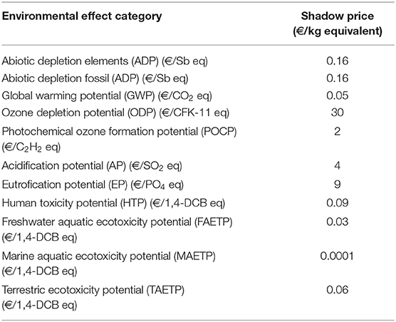
Table 2. Environmental effect categories and shadow prices (TNO-MEP, 2004).

The total environmental costs can then be determined using (Equation 13). Environmental costs incurred during the life cycle of the bridge are not discounted as recommended by Hellweg et al. (2003).

$\begin{array}{ll}EC={\displaystyle \sum _{i=1}^n}{EE}_i\times {SP}_i& (13)\end{array}$

Wherein:

EC = environmental costs (€/functional unit), where a functional unit can be a structural element or the whole structure (e.g., a bridge)

EE_i = environmental effects for impact category i [kg of impact category equivalent (IC_eq)/functional unit (one bridge)]

SP_i = the shadow price for environmental effect category i (€/kg of IC_eq), given in Table 2.

i = environmental impact category for i = 1 until n

The environmental effects per impact category can be determined by Equation (14) as follows:

$\begin{array}{ll}{EE}_i={\displaystyle \sum _{j=1}^n}{EE}_{i,j}\times {Mq}_j& (14)\end{array}$

Wherein:

EE_i = environmental effects for impact category i [kg of impact category equivalent (kg IC_eq)/functional unit (one bridge)]

EE_{i, j} = environmental effect for impact category i per kg of material j (kg ICeq/kg material) given in Table 1

M_qj = material quantity per functional unit for material j (kg material/functional unit)

j = the different materials for j = 1 to n.

Results and Discussion

The developed Whole Life Cycle Cost model was validated on a case study bridge in the Port of Rotterdam described in section Case Study Description. Four different investment and maintenance cases were analyzed within the case study, for a period of 100 years, combining the four scenarios described in the reliability analysis of section Impact on Reliability Level. The life cycle cases were based on the results of the reliability analysis and can be described as follows.

• LC case 1—scenario 1 “do minimum” is performed until the year 2040, followed by scenario 4, “new bridge.”

• LC case 2—scenario 2, “additional maintenance” (strengthening) is first performed. This is followed by scenario 4, “new bridge,” after 20 years. The “do minimum” scenario is also employed in this case during the 20-year period, however the frequency of welding is less than in LC case 1.

• LC case 3—Scenario 1, “do minimum,” and scenario 3, “temporary bridge,” are performed in parallel immediately and considered for a period of 10 years. After 10 years scenario 4, “new bridge,” is employed.

• LC case 4—Scenario 4 “new bridge” is performed immediately so the comparison with the other cases can be established.

The WLCC model considers both direct and indirect costs. The aim of the model is to provide to inform the infrastructure owner about the impacts of different maintenance strategies and enable optimal decision making. Within the model, input parameters can be changed according to the decisions made. The traffic flow scenario Conservative Carbon or Business As usual has been assumed with a value of time equal to 9.92 EUR for passengers commuting by car, and 49.57 EUR for freight traffic (de Jong, 2013). The traffic regulations put in place and the duration of the maintenance activities are as specified by the owner (Rijkswaterstaat, 2016), and prediction of the future performance is based on a combination of historical data and the reliability fatigue model (van der Tuin et al., 2020).

The sensitivity analysis was used to investigate how changes in discount factor influence direct costs. The effect of a 1% change in both directions, meaning discount factors of 0.5% and 2.5%, were analyzed. The analysis revealed that variations in the discount factor highly influence the effect of future cost flows and the final result at different time intervals. For example, for case 2 discount factor of 0.5% result in 32% higher costs at the end of the analyzed period of 100 years, while discount factor of 2.5% gives 26% lower costs for the same period. For the results presented here taken into consideration local economy, a discount rate of 1.5%, has been used. This rate may not be indicative of the discount rate in the Netherlands but was considered acceptable for the purposes of this investigation.

The diagrams in Figure 13 present the results of the developed life cycle cost model. The figures clearly show that different investment and maintenance strategies result in significantly different total costs, but also different impacts of each cost category per strategy. When looking at the direct agency costs, including construction, maintenance and repair, case 2 (including strengthening, thus avoiding construction of the temporary bridge) gives the lowest value. Case 1 (welding scenario) and case 4 (new bridge) come relatively close to the lowest valued case regarding direct costs, while case 3 (temporary bridge) stands out significantly with a much higher whole life cycle cost at the end of the analyzed period. User delay costs are lowest for case 4 “new bridge” since in this case the bridge would be built while the existing bridge is in use which would minimize the influence on existing traffic flows. Case 1 “do minimum” causes the highest user delay costs since it requires frequent inspections and welding treatments. The results regarding total environmental cost (including environmental impact of the construction materials used for activities and impact of traffic delays through increased CO₂ emission) show that cases 2 and 4 have almost the same impact after a longer period of time (lines are overlapping after ~20 years). Environmental costs for case 3 “temporary bridge” are again much higher than the other cases.

FIGURE 13

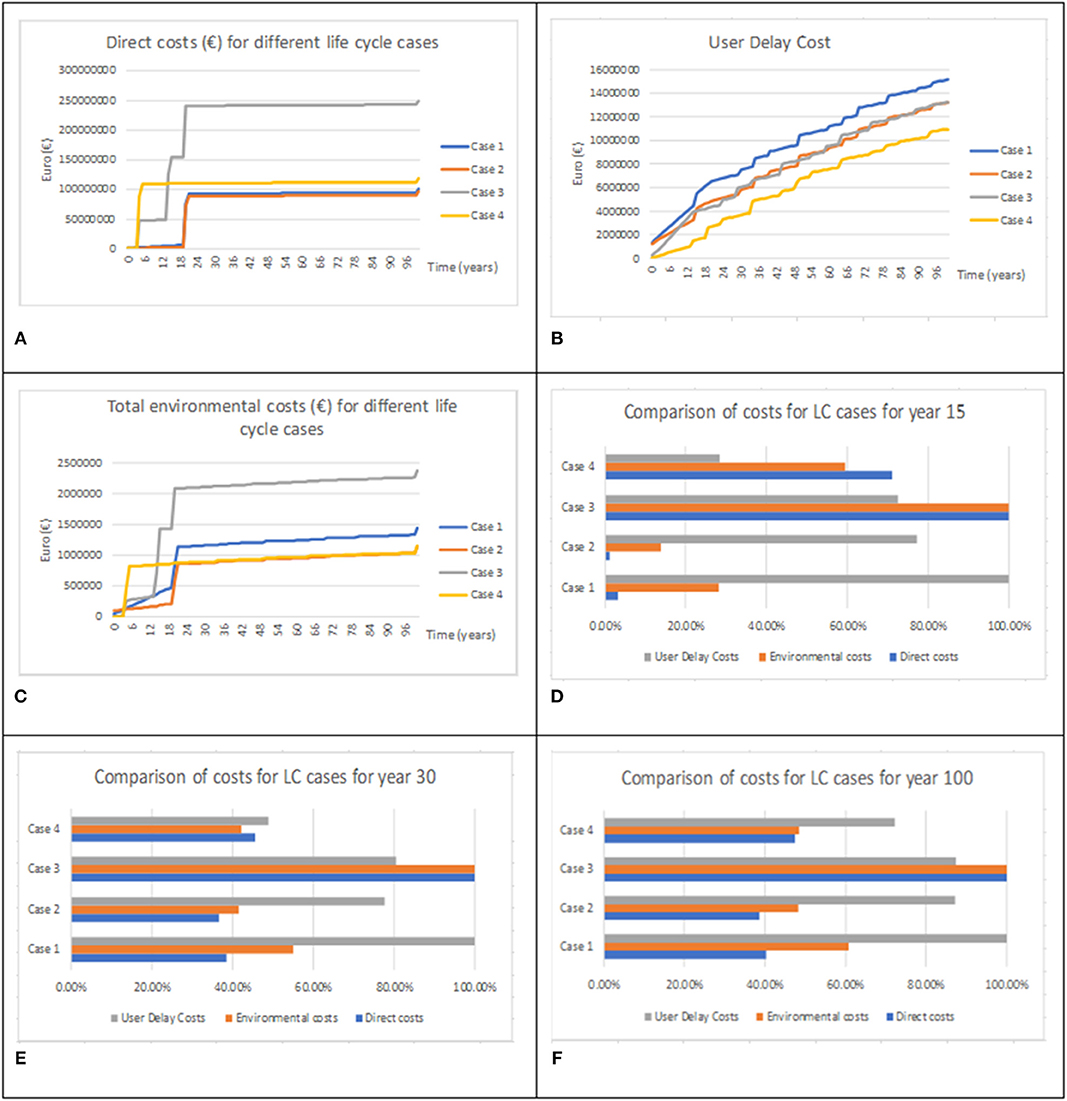
Figure 13. (A) Direct costs, (B) User delay costs (sum of freight and passengers traffic delay costs), (C) Environmental costs (sum of environmental cost regarding materials and environmental impact due to the CO₂ emission regarding traffic delays) for 4 different life cycle cases; and Comparison of costs per category in (D) after 15 years, (E) after 30 years, (F) after 100 years as a relative values.

Comparison of costs for the four different life cycle cases show that the situation changes when the results are presented over time. From direct maintenance and construction costs and environmental cost, case 2 (strengthening option, avoiding temporary bridge) gives the lowest value, while when we also consider user costs, case 1 (welding scenario) is very close to the best value. In all three cost categories case 3, which includes building a temporary bridge, gives the highest value when analyzed for both short and long time periods. The option of building a new bridge now, scenario 4, is not economically the most viable, but from the user's perspective it is the best option. It seems that the benefit, including the increased safety should be considered in future practice. For example, if the risk of bridge collapse is 1%, but the associated monetised delay and renovation costs are much higher than 1% of the costs associated with preventative renovation works, the infrastructure owner may decide to invest money in renovating the bridge.

Conclusion

Transport infrastructure managers are currently facing critical issues, such as decreasing annual maintenance budgets, aging infrastructure, as well as climate change impacts. The purpose of the reliability-based life cycle management model presented is to satisfy the required reliability performance, while considering economic, societal, and environmental impacts of different maintenance strategies. The lifecycle model uses the outputs from a reliability model and a traffic flow model, taking the multi-modal nature of the transport network into account in order to determine the impacts of closures or any disruptions. The model presented in this paper has been implemented on a case study bridge in the Port of Rotterdam in the Netherlands, representing one of the critical links on the multi-modal network. The main problem for the selected bridge is cracking due to fatigue. Fatigue damage is a common issue in steel orthotropic decks, which for the current structure has been aggravated by the significant traffic growth since the bridge was designed, including significant freight increases. Thus, calculation of the reliability of the structure was required with respect to the Fatigue Limit State. Based on the inspection and modeling results, it has been decided that the bridge needs significant rehabilitation and strengthening, and therefore four different management scenarios have been analyzed. For each maintenance scenario the reliability levels have been determined and optimized, in order to maintain bridge safety, while the life cycle cost model calculated the direct and indirect impacts of different interventions. This case study has shown that by employing traffic modeling and associating monetary values to societal and environmental impacts as consequences of different maintenance and investment options, infrastructure managers can make better-informed decisions regarding maintenance planning.

Data Availability Statement

The datasets generated for this study are available on request to the corresponding author.

Author Contributions

IS and LC designed the model. IS structured the paper and wrote the sections Introduction, Case study description, Whole life cycle cost model, Results and discussion, and Conclusion. SS made all LCC calculations and graphics. LC, RD, and IB performed bridge modeling. All authors together developed lice cycle management scenarios.

Conflict of Interest

LC, MD, RD, and IB were employed by the company Roughan & O'Donovan Ltd.

The remaining authors declare that the research was conducted in the absence of any commercial or financial relationships that could be construed as a potential conflict of interest.

Acknowledgments

This work has been a part of SAFE-10-T project, which has received funding from the European Union's Horizon 2020 research and innovation programme under grant agreement No 723254. We acknowledge Netherlands Ministry of Infrastructure and Environment (Rijkswaterstaat) for provision of data and digital and analog visual material.

References

AASHTO (1990). Guide Specifications for Fatigue Evaluation of Existing Steel Bridges. Washington DC: American Association of State Highway and Transportation Officials.

Adasooriya, N. D. (2016). Fatigue reliability assessment of ageing railway truss bridges: rationality of probabilistic stress-life approach. Case Stud. Struct. Eng. 6, 1–10. doi: 10.1016/j.csse.2016.04.002

CrossRef Full Text | Google Scholar

Allah Bukhsh, Z., Stipanovic, I., Klanker, G. O., Connor, A., and Doree, A. G. (2019). Network level bridges maintenance planning using multi-attribute utility theory. Struct. Infrastruct. Eng. 15, 872–885. doi: 10.1080/15732479.2017.1414858

CrossRef Full Text | Google Scholar

ASCAM (2012). Asset Service Condition Assessment Methodology Deliverable No.3 Inventory Bridge Management practices Final Report. Available online at: http://www.cedr.eu/download/other_public_files/research_programme/eranet_road/call_2010_asset_management/ascam/ASCAM-R3-final-reportN.PDF

Brühwiler, E. (2019). UHPFRC technology to enhance the performance of existing concrete bridges. Struct. Infrastruct. Eng. 16, 1–12. doi: 10.1080/15732479.2019.1605395

CrossRef Full Text | Google Scholar

Brühwiler, E., and Denarié, E. (2013). Rehabilitation and strengthening of concrete structures using ultra-high performance fibre reinforced concrete. Struct. Eng. Int. 23, 450–457. doi: 10.2749/101686613X13627347100437

CrossRef Full Text | Google Scholar

BSI (1980). BS 5400: Steel, Concrete and Composite Bridges—Part 10: Code of Practice for Fatigue. London: British Standards Institution.

CEN (1992). Eurocode 3: Design of Steel Structures, Part 1–9: Fatigue. Brussels: European Committee for Standardization.

Google Scholar

Chryssanthopoulos, M. K., and Righiniotis, T. D. (2006). Fatigue reliability of welded steel structures. J. Construct. Steel Res. 62, 1199–1209. doi: 10.1016/j.jcsr.2006.06.007

CrossRef Full Text | Google Scholar

Davis Langdon Management Consulting (2014). Life Cycle Costing (LCC) as a Contribution to Sustainable Construction. Guidance Document. Ref. Ares (2014) 1138398.

de Bruyn, S., Korteland, M., Markowska, A., Davidson, M., de Jong, F., Bles, M., and Sevenster, M. (2010). Valuation and weighting of emissions and environmental impacts. Shadow Prices Handbook. Available online at: https://www.cedelft.eu/publicatie/shadow_prices_handbook_:_valuation_and_weighting_of_emissions_and_environmental_impacts/1032

de Jong, G. (2013). International Comparison of Transport Appraisal Practice, Annex 3 The Netherlands Country Report Project Funded by the Department for Transport, UK, Institute for Transport Studies. Available online at: http://ec.europa.eu/transport/themes/its/road/action_plan/doc/2012-its-plan-the-netherlands-2013-2017.pdf

Denarié, E., Habert, G., and Sajna, A. (2009). Recommendations for the Use of UHPFRC in Composite Structural Members. Rehabilitation Log Cezsoški bridge. ARCHES deliverable D14.

Google Scholar

Det Norske Veritas (DNV) (2010). Fatigue Design of Offshore Steel Structures, No. DNV-RP-C203.

Google Scholar

EN 1991-2 (2003). Eurocode 1: Actions on Structures – Part 2: Traffic Loads on Bridges. Brussels: European Standard; CEN.

European Commission (2018). Rhine Alpine TEN-T Core Network Corridor, Work Plan of the Coordinator. Available online at: https://ec.europa.eu/transport/sites/transport/files/3rd_workplan_ralp.pdf

European Commission (2019). State of Infrastructure Maintenance, Discussion Paper, Directorate-General for Internal Market, Industry, Entrepreneurship and SMEs, Industrial Transformation and Advance Value Chains, Clean Technologies and Products. Available online at https://ec.europa.eu/docsroom/documents/34561/attachments/1/translations/en/renditions/native (accessed April 06, 2020).

European Railway Agency (2014). Railway Safety Performance in the European Union 2014, 82. Available online at: http://www.era.europa.eu/Document-Register/Documents/SPR2014.pdf

FHWA (2019). Report on Techniques for Bridge Strengthening. U.S. Department of Transportation – Federal Highway Administration, Main Report, FHWA-HIF-18-041. Available online at: https://www.fhwa.dot.gov/bridge/pubs/hif18041.pdf (accessed April 08, 2020).

FIEC (2018). Crucial Maintenance of Transport Infrastructure, Construction Europe. Available online at: https://www.fiec-ar.eu/images/pdf/ECO-Maintenance%20of%20Infrastructure-Construction%20Europe-FIEC%20article.pdf (accessed April 3, 2020).

Forzieri, G., Bianchi, A., Marin Herrera, M. A., Batista e Silva, F., Feyen, L., and Lavalle, C. (2015). Resilience of Large Investments and Critical Infrastructures in Europe to Climate Change. EUR 27598 EN. Luxembourg: Publications Office of the European Union.

PubMed Abstract | Google Scholar

Gkoumas, K., Marques Dos Santos, F. L., van Balen, M., Tsakalidis, A., Ortega Hortelano, A., Grosso, M., et al. (2019a). Research and Innovation in Bridge Maintenance, Inspection and Monitoring - A European Perspective Based on the Transport Research and Innovation Monitoring and Information System (TRIMIS). EUR 29650 EN. Luxembourg: Publications Office of the European Union.

Google Scholar

Gkoumas, K., van Balen, M., Ortega Hortelano, A., Tsakalidis, A., Grosso, M., Haq, G., and Pekár, F. (2019b). Research and Innovation in Transport Infrastructure - An Assessment Based on the Transport Research and Innovation Monitoring and Information System (TRIMIS). EUR 29829 EN. Luxembourg: Publications Office of the European Union.

Google Scholar

Hajializadeh, D., Leahy, C., Connolly, L., and O'Connor, A. (2015). Weight Limits for Non-Regulated HGVs: Data Cleaning Report. Transport Infrastructure Ireland.

Hegger, S., and de Graaf, D. (2013). Vergelijkende LCA studie bruggen (in Dutch, LCA Comparative Study of Bridges). Rotterdam: BECO.

Hellweg, S., Hofstetter, T. B., and Hungerbuhler, K. (2003). Discounting and the environment should current impacts be weighted differently than impacts harming future generations? Int. J. Life Cycle Assess. 8, 8–18. doi: 10.1007/BF02978744

CrossRef Full Text | Google Scholar

Huang, T.-L., Zhou, H., Chec, H.-P., and Ren, W.-X. (2016). Stochastic modelling and optimum inspection and maintenance strategy for fatigue affected steel bridge members. Smart Struct. Syst. 18, 569–584. doi: 10.12989/sss.2016.18.3.569

CrossRef Full Text | Google Scholar

Hurt, M., and Schrock, S. (2016). Highway Bridge Maintenance Planning and Scheduling. Amsterdam: Elsevier. Retrieved from https://www.sciencedirect.com (accessed April 7, 2020).

ISO 2394 (2015). General Principles on Reliability for Structures.

JCSS (2001). Probabilistic Assessment of Existing Structures-A Publication for the Joint Committee on Structural Safety (JCSS). Vol. 32. RILEM Publications.

Google Scholar

Kwon, K., and Frangopol, D. M. (2010). Bridge fatigue reliability assessment using probability density functions of equivalent stress range based on field monitoring data. Int. J. Fatigue 32, 1221–1232. doi: 10.1016/j.ijfatigue.2010.01.002

CrossRef Full Text | Google Scholar

Kwon, K., Frangopol, D. M., and Soliman, M. (2012). Probabilistic fatigue life estimation of steel bridges by using a bilinear S-N approach. J. Bridge Eng. 17, 58–70. doi: 10.1061/(ASCE)BE.1943-5592.0000225

CrossRef Full Text | Google Scholar

Lee, Y.-J., Kim, R. E., Suh, W., and Park, K. (2017). probabilistic fatigue life updating for railway bridges based on local inspection and repair. Sensors 17:936. doi: 10.3390/s17040936

PubMed Abstract | CrossRef Full Text | Google Scholar

Melchers, R. E., and Beck, A. T. (2018). Structural Reliability Analysis and Prediction. Hoboken, NJ: John Wiley and Sons. doi: 10.1002/9781119266105

CrossRef Full Text | Google Scholar

Miner, M. A. (1945). Cumulative damage in fatigue. J. Appl. Mech. 12, 159–164.

Moreu, F., Li, X., Li, S., and Zhang, D. (2018). Technical specifications of structural health monitoring for highway bridges: new chinese structural health monitoring code. Front. Built Environ. 4:10. doi: 10.3389/fbuil.2018.00010

CrossRef Full Text | Google Scholar

Moy, S. S. J., and Bloodworth, A. G. (2007). Strengthening a steel bridge with CFRP composites. Proc. Inst. Civil Eng. Struct. Build. 160, 81–93. doi: 10.1680/stbu.2007.160.2.81

CrossRef Full Text | Google Scholar

New York Times (2019). Bridge disasters – Times Topic. The New York Times. Available online at: https://www.nytimes.com/topic/subject/bridge-disasters, (accessed December 8, 2019).

O'Brien, E. J., and Enright, B. (2011). Modeling same-direction two-lane traffic for bridge loading. Struct. Saf. 33, 296–304. doi: 10.1016/j.strusafe.2011.04.004

CrossRef Full Text | Google Scholar

Ortúzar, J., and Willumsen, L. (2011). Modelling Transport, 4th Edn. John Wiley. doi: 10.1002/9781119993308

CrossRef Full Text | Google Scholar

Pastori, E. (2015). Modal Share of Freight Transport to and From EU ports. Policy Depatment B: Structural and Cohesion Policies - Transport and Tourism, 53.

Patidar, V., Labi, S., Sinha, K. C., and Thompson, P. (2007). Multi-Objective Optimization for Bridge Management Systems. NCHRP REPORT 590.

Google Scholar

Port of Rotterdam (2018). Facts and Figures. Available online at: https://www.portofrotterdam.com/en/our-port/facts-figures-about-the-port

Port of Rotterdam Authority (2019). Highlights of the 2018 Annual Report. Available online at: https://www.portofrotterdam.com/en/port-authority/about-the-port-authority/finance/annual-reports

Rijkswaterstaat (2016). Ideeën marktparticipatie 5 september 2016: Tijdelijke brug in combinatie met de bestaande brug. Marktparticipatie Suurhoffbrug 31121821, Infopakket. Available online at: https://www.tenderned.nl/tenderned

Sahrapeyma, A., Hosseini, A., and Marefat, M.-S. (2013). Life-cycle prediction of steel bridges using reliability-based fatigue deterioration profile: case study of neka bridge. Int. J. Steel Struct. 13, 229–242 doi: 10.1007/s13296-013-2003-8

CrossRef Full Text | Google Scholar

Schultz van Haegen, M. H. (2017). Startbeslissing Suurhoffbrug. Ministry of Infrastrcuture and Environment (Rijkswaterstaat). IENM/BSK-2017/194295. Available online at: https://www.suurhoffbrug.nl/documenten/besluiten/2017/10/12/rapportage-startbeslissing-suurhoffbrug.

Skaric Palic, S., and Stipanovic, I. (2019). SAFE-10-T Deliverable D2.4 Report on Whole Life Cycle Model. Available online at: www.safe10tproject.eu

Stipanovic, I., Chatzi, E., Limongelli, M., Gavin, K., Allah Bukhsh, Z., Skaric Palic, S., et al. (2017). Working Group 2 Report: Performance Goals for Roadway Bridges of Cost Action TU1406.

Google Scholar

Sundquist, H., and Karoumi, R. (2012). Life Cycle Cost Methodology and LCC Tools. ETSI. Available online at: http://www.etsi.aalto.fi/Etsi3/PDF/TG3/LCC%20Description.pdf

Google Scholar

Tavasszy, L. (2006). “Freight Modeling - An overview of International Experiences,” in TRB Conference on Freight Demand Modelling: Tools for Public Sector Decision Making (Washington, DC).

Thinkstep (2015). Description of the CML 2001 Method. Available online at: http://www.gabisoftware.com/support/gabi/gabi-lcia-documentation/cml-2001/

Van Dam, K. H., Nikolic, I., and Lukszo, Z. (2012). Agent-Based Modelling of Socio-Technical Systems, Vol. 9. Springer Science and Business Media. doi: 10.1007/978-94-007-4933-7

CrossRef Full Text | Google Scholar

van der Tuin, M., and Pel, A. J. (2019). SAFE-10-T Deliverable D2.2 Report on Network Model. Available online at: www.safe10tproject.eu

van der Tuin, M. S., Connolly, L., Donnelly, R., Stipanovic, I., Skaric Palic, S, Hajdin, R., et al. (2020). SAFE-10-T Deliverable D4.1 Report on the Results of Case Study 1 - the Netherlands. Available online at: www.safe10tproject.eu

Google Scholar

van der Velde, J., Klatter, L., and Bakker, J. (2013). A holistic approach to asset management in the Netherlands. Struct. Infrastruct. Eng. 9, 340–348. doi: 10.1080/15732479.2012.657650

CrossRef Full Text | Google Scholar